
Implementation of a High-Sensitivity Global Navigation Satellite System Receiver on a System-on-Chip Field-Programmable Gate Array Platform


Abstract
1. Introduction
1.1. Motivation
1.2. Contributions
1.3. Organization of the Paper
2. Literature Review
3. System Design
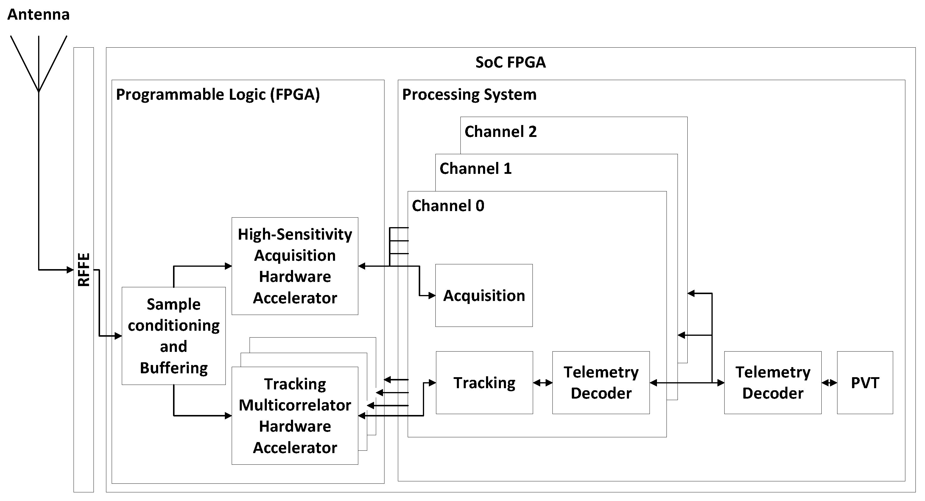
3.1. High Sensitivity GNSS Receiver Architecture
3.2. Receiver Operating Modes
3.3. Assistance Data
3.4. Acquisition in High-Sensitivity Mode
3.4.1. Theory of Operation
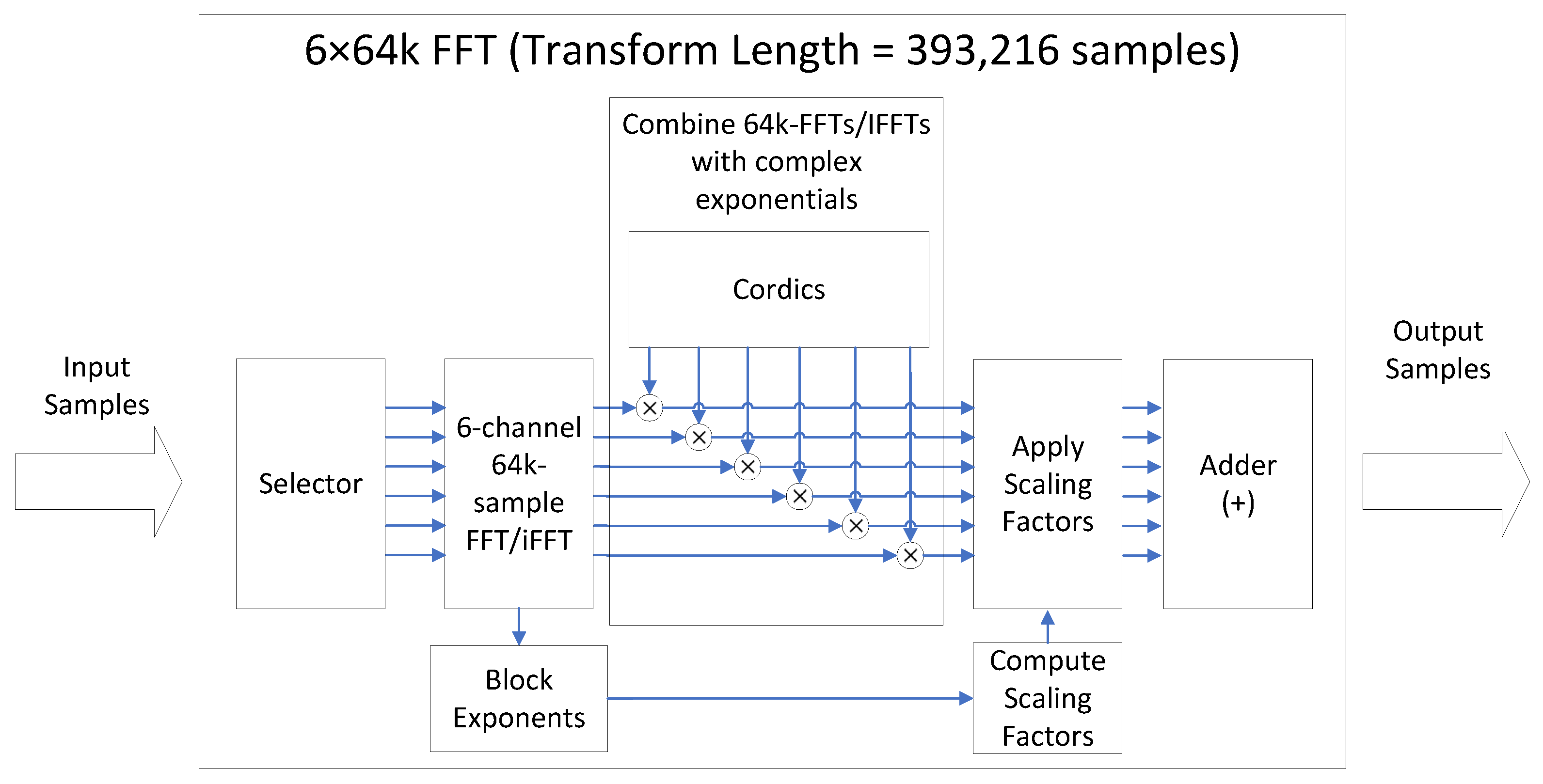
3.4.2. Computation of Large FFTs in the FPGA
- The sampling frequency is chosen so that the number of samples N representing 100 ms is a multiple, P, of a power of two. is constrained to be a power of two to ensure compatibility with FFT IP cores provided by FPGA manufacturers.
- To minimize the computation overhead in the proposed implementation, is set to its maximum feasible value. This value is determined by either the maximum transform length supported by the FFT IP cores from FPGA manufacturers or a value that ensures the sampling frequency is as close as possible to the desired value.
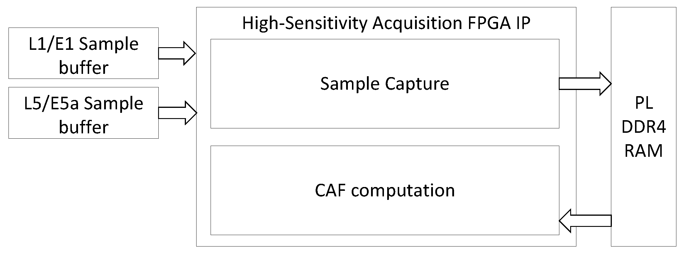
3.4.3. Implementation
| Algorithm 1 High-sensitivity acquisition |
|
- 1.
- In the first step, the CAF computation module computes the frequency domain representation of the circular correlation: the module fetches 100 ms of samples from the PL memory component, performs Doppler wipeoff, computes the FFT of the Doppler-corrected signal, and multiplies the results by the FFT of the local replica of the pilot tiered code. Finally, the result of this multiplication is stored back into the PL memory component. Storing intermediate results in the PL memory component reduces FPGA memory usage. During this first step, the Enable/Disable Doppler wipeoff block and the Enable/Disable FFT Multiplication block shown in Figure 8 are enabled. The local carrier used for Doppler wipeoff is efficiently implemented using the Coordinate Rotation Digital Computer (CORDIC) algorithm [38].
- 2.
- In the second step, the CAF computation module calculates the time-domain representation of the circular cross-correlation. It retrieves the results of the multiplication of the FFT by the local replica obtained in step 1, performs the IFFT, and then stores the results back in the PL memory component.
3.5. Doppler Prediction
3.6. Acquisition in Normal-Sensitivity Mode
3.7. Tracking
3.7.1. Tracking in High-Sensitivity Mode
3.7.2. Tracking in Normal-Sensitivity Mode
3.8. Telemetry Decoding
3.8.1. Sync Frame Detection
3.8.2. Sync Frame Confirmation
3.8.3. TOW Estimation
3.9. Computation of the Navigation Solutions
3.10. GNSS Output Products
4. Results
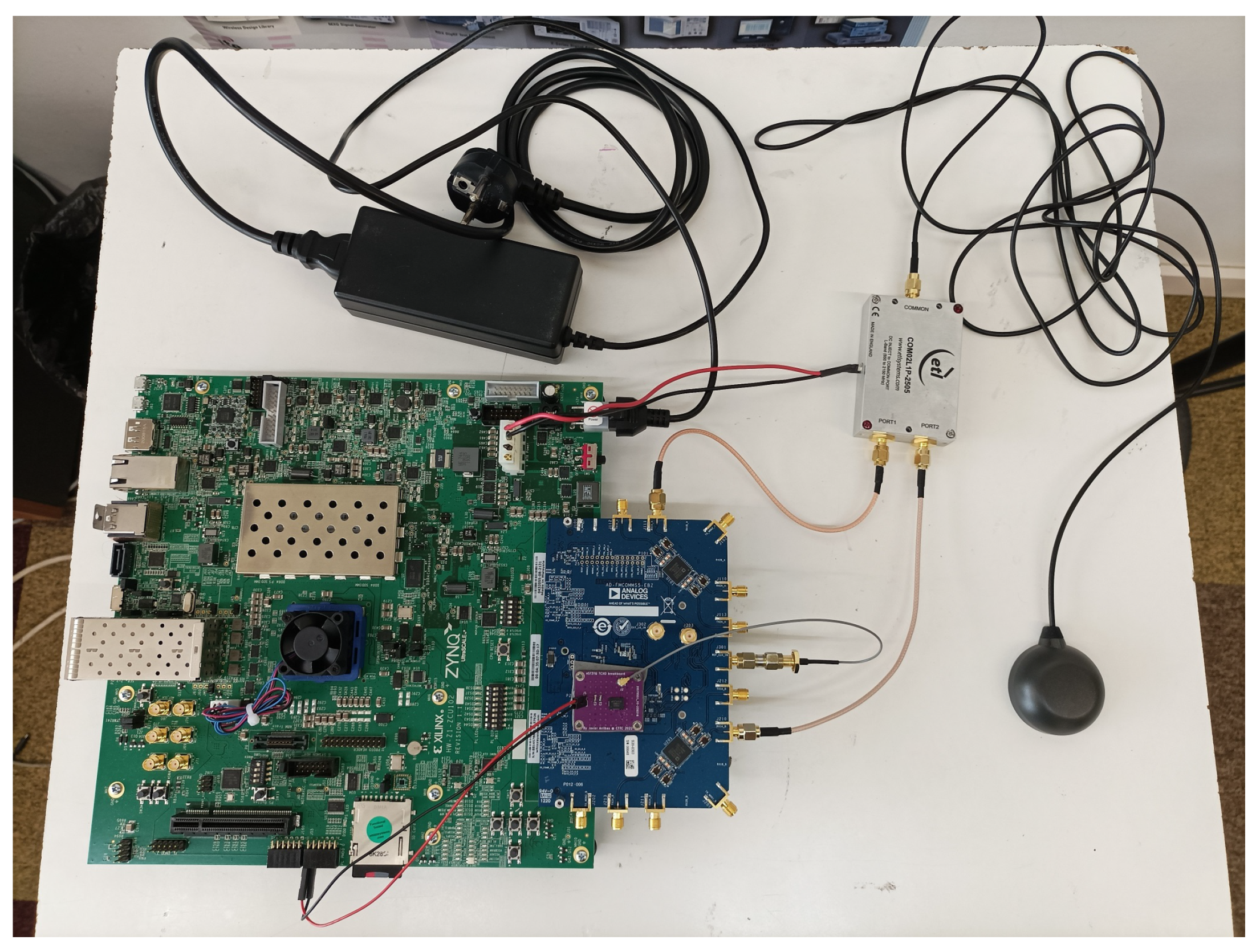
4.1. Test Setup
4.2. High-Sensitivity Acquisition Latency
4.2.1. Tests Results Using the TCXO
4.2.2. Tests Results Using the OCXO
4.3. Acquisition and Tracking of GNSS Signals in Real Time
4.3.1. Tests Results Using GPS and Galileo Signals at Nominal Power Levels
4.3.2. Tests Results Using Weak Galileo E1b/c Signals
4.4. Precision of the Navigation Solutions
4.4.1. Tests Results Using GPS and Galileo Signals at Nominal Power Levels
4.4.2. Tests Results Using Weak Galileo E1b/c Signals
4.5. Estimated Power Consumption
5. Conclusions
Author Contributions
Funding
Institutional Review Board Statement
Informed Consent Statement
Data Availability Statement
Conflicts of Interest
Abbreviations
| GNSS | Global Navigation Satellite System |
| HS | High Sensitivity |
| SoC-FPGA | System-on-Chip Field-Programmable Array |
| SDR | Software Defined Radio |
| Carrier to noise density ratio | |
| A-GNSS | Assisted GNSS |
| CI | Coherent Integration |
| GPS | Global Positioning System |
| PRN | Pseudo Random Noise |
| SNR | Signal to Noise Ratio |
| TCXO | Temperature-Compensated Crystal Oscillator |
| OCXO | Oven Controlled Crystal Oscillator |
| NCI | Non-Coherent Integration |
| PDI | Post-Detection Integration |
| FFT | Fast Fourier Transform |
| DBZP | Double BLock Zero Padding |
| LBS | Location-Based Services |
| TTFF | Time to First Fix |
| NPDI | Non-coherent Post Detection Integration |
| DPDI | Differential Post-Detection Integration |
| GPDIT | Generalized Post-Detection Integration Truncated |
| SD | Squaring Detector |
| GPDITSD | GPDIT and SD |
| CSAC | Chip Scale Atomic CLock |
| PCPS | Parallel Code Phase Search |
| IFFT | Inverse Fast Fourier Transform |
| IP | Intellectual Property |
| RFFE | Radio Frequency Front-End |
| OS | Operating System |
| AMD | Advanced Micro Devices |
| MPSoC | Multi-Processor System-on-Chip |
| PL | Processing Logic |
| PS | Processing System |
| MPCore | MultiProcessor Core |
| PVT | Position, Velocity, and Time |
| LAN | Local Area Network |
| RF | Radio Frequency |
| ppm | parts per million |
| ppb | parts per billion |
| AMBA | Advanced Microcontroller Bus Architecture |
| AXI4 | Advanced eXtensible Interface |
| DMA | Direct Memory Access |
| DDR4 | Double Data Rate 4 |
| COTS | Commercial off-the-shelf |
| PCB | Printed Circuit Board |
| UTC | Coordinated Universal Time |
| XML | Extensible Markup Language |
| TOW | Time Of Week |
| CAF | Cross Ambiguity Function |
| DFT | Discrete Fourier Transform |
| CFAR | Constant False Alarm Rate |
| GLRT | Generalized Likelihood Ratio Test |
| CORDIC | Coordinate Rotation Digital Computer |
| Msps | Mega samples per second |
| CFO | Carrier Frequency Offset |
| DLL | Delay-Locked Loop |
| PLL | Phase-Locked Loop |
| VEMLP | Very Early Minus Very Late Power |
| TOA | Time of Arrival |
| GST | Galileo System Time |
| NTP | Network Time Protocol |
| WAN | Wide Area Network |
| GDOP | Geometric Dilution of Precision |
| RAIM-FDE | Receiver Autonomous Integrity Monitoring Failure Detection and Exclusion |
| RINEX | Receiver Independent Exchange Format |
| RTCM | Radio Technical Commission for Maritime Services |
| NMEA | National Marine Electronics Association |
| WGS-84 | World Geodetic System 1984 |
| DOP | Dilution of precision |
| LNA | Low Noise Amplifier |
| DRMS | Distance Root Mean Square |
| CEP | Circular Error Probability |
| SAS | Spherical Accuracy Standard |
| MRSE | Mean Radial Spherical Error |
| SEP | Spherical Error Probable |
| ENU | East–North–Up |
Appendix A
Appendix A.1

| Signal | Parameter | Value |
|---|---|---|
| Acquisition Galileo E1b/c | CI time Max NCI combinations Doppler prediction 1st stage acq: Doppler max 1st stage acq: Doppler step 2nd stage acq: Doppler max 2nd stage acq: Doppler step PFA Downsampling factor | 100 ms 7 Enabled 50 Hz 5 Hz 10 Hz 5 Hz 4 |
| Signal | Parameter | Value |
|---|---|---|
| Tracking Galileo E1b/c | Coherent integration time Early–Late space narrow chips Very Early–Late space narrow chips PLL filter bandwidth (narrow correlator) DLL filter bandwidth (narrow correlator) | 40 ms chips chips 5 Hz Hz |
Appendix A.2
| Signal | Parameter | Value |
|---|---|---|
| Acquisition GPS L1 C/A | CI time Max NCI combinations Doppler max Doppler step PFA Downsampling factor | 1 ms 4 5000 Hz 250 Hz 4 |
| Acquisition GPS L5 | CI time Max NCI combinations Assistance to secondary band Doppler max Doppler step PFA | 1 ms 4 enabled 500 Hz 250 Hz |
| Acquisition Galileo E5a | CI time Max NCI combinations Assistance to secondary band Doppler max Doppler step PFA Downsampling factor | 1 ms 4 enabled 500 Hz 250 Hz 4 |
| Signal | Parameter | Value |
|---|---|---|
| Tracking GPS L1 C/A | Coherent integration time Early–Late space chips Early–Late space narrow chips PLL filter bandwidth PLL filter bandwidth (narrow correlator) DLL filter bandwidth DLL filter bandwidth (narrow correlator) | 20 ms chips chips 35 Hz Hz 2 Hz Hz |
| Tracking GPS L5 | Coherent integration time Early–Late space chips Early–Late space narrow chips PLL filter bandwidth PLL filter bandwidth (narrow correlator) DLL filter bandwidth DLL filter bandwidth (narrow correlator) | 20 ms chips chips 20 Hz Hz Hz Hz |
| Tracking Galileo E5a | Coherent integration time Early–Late space chips Early–Late space narrow chips PLL filter bandwidth PLL filter bandwidth (narrow correlator) DLL filter bandwidth DLL filter bandwidth (narrow correlator) | 20 ms chips chips 20 Hz Hz Hz Hz |
Appendix A.3
| Type of Configuration | Parameter | Value |
|---|---|---|
| General | Positioning Mode RAIM FDE Iono Model Trop Model PVT Output Rate Use unhealthy sats | Single Enabled Broadcast Saastamoinen 1 s Disabled |
| PVT Kalman Filter | Standard deviation of the position estimations Std. dev. of the velocity estimations Std. dev. of the dynamic system model for pos. Std. dev. of the dynamic system model for vel. | 1 m m/s m m/s |
References
- Ren, T.; Petovello, M.G. A Stand-Alone Approach for High-Sensitivity GNSS Receivers in Signal-Challenged Environment. IEEE Trans. Aerosp. Electron. Syst. 2017, 53, 2438–2448. [Google Scholar] [CrossRef]
- Van Diggelen, F. A-GPS: Assisted GPS, GNSS, and SBAS; Artech: Norwood, MA, USA, 2009. [Google Scholar]
- Seco-Granados, G.; López-Salcedo, J.; Jiménez-Baños, D.; López-Risueño, G. Challenges in Indoor Global Navigation Satellite Systems: Unveiling its core features in signal processing. IEEE Signal Process. Mag. 2012, 29, 108–131. [Google Scholar] [CrossRef]
- Marathe, T.; Broumandan, A.; Pirsiavash, A.; Lachapelle, G. Characterization of Range and Time Performance of Indoor GNSS Signals. In Proceedings of the 2018 European Navigation Conference (ENC), Gothenburg, Sweden, 14–17 May 2018; pp. 27–37. [Google Scholar] [CrossRef]
- Renaudin, V.; Yalak, O.; Tomé, P. Hybridization of MEMS and Assisted GPS for Pedestrian Navigation. Inside GNSS, 1 January 2007; pp. 34–42. [Google Scholar]
- Egea-Roca, D.; Arizabaleta-Diez, M.; Pany, T.; Antreich, F.; López-Salcedo, J.A.; Paonni, M.; Seco-Granados, G. GNSS User Technology: State-of-the-Art and Future Trends. IEEE Access 2022, 10, 39939–39968. [Google Scholar] [CrossRef]
- Gómez-Casco, D. Non-Coherent Acquisition Techniques for High-Sensitivity GNSS Receivers. Ph.D. Thesis, Universitat Autònoma de Barcelona, Barcelona, Spain, 2018. [Google Scholar]
- Jiménez-Baños, D.; Blanco-Delgado, N.; López-Risueño, G.; Seco-Granados, G.; Garcia-Rodríguez, A. Innovative Techniques for GPS Indoor Positioning Using a Snapshot Receiver. In Proceedings of the 19th International Technical Meeting of the Satellite Division of The Institute of Navigation (ION GNSS 2006), Fort Worth, TX, USA, 26–29 September 2006; pp. 2944–2955. [Google Scholar]
- Lucas Sabola, V.; Seco Granados, G.; Lopez Salcedo, J.; García-Molina, J. GNSS IoT Positioning: From Conventional Sensors to a Cloud-Based Solution. Inside GNSS. 15 June 2018. Available online: https://insidegnss.com/gnss-iot-positioning-from-conventional-sensors-to-a-cloud-based-solution/ (accessed on 18 February 2024).
- European GNSS Agency. GNSS User Technology Report; Issue 1; Publications Office of European Union: Luxembourg, 2016. [Google Scholar] [CrossRef]
- Domínguez, E.; Pousinho, A.; Boto, P.; Gómez-Casco, D.; Locubiche-Serra, S.; Seco-Granados, G.; López-Salcedo, J.A.; Fragner, H.; Zangerl, F.; Peña, O.; et al. Performance Evaluation of High Sensitivity GNSS Techniques in Indoor, Urban and Space Environments. In Proceedings of the 29th International Technical Meeting of the Satellite Division of The Institute of Navigation (ION GNSS+ 2016), Portland, OR, USA, 12–16 September 2016; pp. 373–393. [Google Scholar] [CrossRef]
- Gómez-Casco, D.; López-Salcedo, J.A.; Seco-Granados, G. Generalized integration techniques for high-sensitivity GNSS receivers affected by oscillator phase noise. In Proceedings of the 2016 IEEE Statistical Signal Processing Workshop (SSP), Palma de Mallorca, Spain, 26–29 June 2016; pp. 1–5. [Google Scholar] [CrossRef]
- Lin, D.M.; Tsui, J.B.; Howell, D. Direct P(Y)-Code Acquisition Algorithm forSoftware GPS Receivers. In Proceedings of the 12th International Technical Meeting of the Satellite Division of The Institute of Navigation (ION GPS 1999), Nashville, TN, USA, 14–17 September 1999; pp. 363–368. [Google Scholar]
- Yang, C.; Hegarty, C.; Tran, M. Acquisition of the GPS L5 Signal Using Coherent Combining of I5 and Q5. In Proceedings of the 17th International Technical Meeting of the Satellite Division of The Institute of Navigation (ION GNSS 2004), Long Beach, CA, USA, 21–24 September 2004; pp. 2184–2195. [Google Scholar]
- Ziedan, N.; Garrison, J. Unaided acquisition of weak GPS signals using circular correlation or double-block zero padding. In Proceedings of the PLANS 2004. Position Location and Navigation Symposium (IEEE Cat. No.04CH37556), Monterey, CA, USA, 26–29 April 2004; pp. 461–470. [Google Scholar] [CrossRef]
- Ziedan, N. Global Navigation Satellite System (GNSS) Receivers for Weak Signals; Artech: Norwood, MA, USA, 2006. [Google Scholar]
- Kong, S.H. High Sensitivity and Fast Acquisition Signal Processing Techniques for GNSS Receivers: From fundamentals to state-of-the-art GNSS acquisition technologies. IEEE Signal Process. Mag. 2017, 34, 59–71. [Google Scholar] [CrossRef]
- Fernández-Prades, C.; Vilà-Valls, J.; Arribas, J.; Ramos, A. Continuous Reproducibility in GNSS Signal Processing. IEEE Access 2018, 6, 20451–20463. [Google Scholar] [CrossRef]
- Fernández-Prades, C.; Arribas, J.; Majoral, M.; Vilà-Valls, J.; García-Rigo, A.; Hernández-Pajares, M. An Open Path from the Antenna to Scientific-grade GNSS Products. In Proceedings of the 6th ESA Intl. Colloquium on Scientific and Fundamental Aspects of GNSS/Galileo, Valencia, Spain, 25–27 October 2017. [Google Scholar]
- Majoral, M.; Fernández-Prades, C.; Arribas, J. Implementation of GNSS Receiver Hardware Accelerators in All-programmable System-On-Chip Platforms. In Proceedings of the 31st International Technical Meeting of the Satellite Division of The Institute of Navigation (ION GNSS+ 2018), Miami, FL, USA, 24–28 September 2018; pp. 4215–4230. [Google Scholar]
- Majoral, M.; Fernández-Prades, C.; Arribas, J. A Flexible System-on-Chip Field-Programmable Gate Array Architecture for Prototyping Experimental Global Navigation Satellite System Receivers. Sensors 2023, 23, 9483. [Google Scholar] [CrossRef] [PubMed]
- Gómez-Casco, D.; López-Salcedo, J.A.; Seco-Granados, G. Optimal fractional non-coherent detector for high-sensitivity GNSS receivers robust against residual frequency offset and unknown bits. In Proceedings of the 2017 14th Workshop on Positioning, Navigation and Communications (WPNC), Bremen, Germany, 25–26 October 2017; pp. 1–5. [Google Scholar] [CrossRef]
- Borre, K.; Akos, D.; Bertelsen, N.; Rinder, P.; Jensen, S. A Software-Defined GPS and Galileo Receiver: A Single-Frequency Approach, 1st ed.; Birkhäuser: Boston, MA, USA, 2007. [Google Scholar] [CrossRef]
- Leclère, J. Resource-Efficient Parallel Acquisition Architectures for Modernized GNSS Signals. Ph.D. Thesis, Swiss Federal Institute of Technology Lausanne, Lausanned, Switzerland, 2014. [Google Scholar] [CrossRef]
- Fernández-Prades, C.; Arribas, J.; Closas, P.; Aviles, C.; Luis, E. GNSS-SDR: An Open Source Tool for Researchers and Developers. In Proceedings of the 24th International Technical Meeting of the Satellite Division of The Institute of Navigation (ION GNSS 2011), Portlan, OR, USA, 20–23 September 2011; pp. 780–794. [Google Scholar]
- GNSS-SDR An Open-Source Global Navigation Satellite Systems Software-Defined Receiver. Available online: https://gnss-sdr.org/ (accessed on 18 February 2024).
- Advanced Micro Devices Inc. ZCU102 Evaluation Board User Guide; UG1182 (v1.7); Advanced Micro Devices Inc.: Santa Clara, CA, USA, 2023. [Google Scholar]
- Advanced Micro Devices Inc. Zynq Ultrascale+ Device Technical Reference Manual; UG1085 (v2.3.1); Advanced Micro Devices Inc.: Santa Clara, CA, USA, 2023. [Google Scholar]
- Analog Devices Inc. AD-FMCOMMS5-EBZ User Guide. Available online: https://wiki.analog.com/resources/eval/user-guides/ad-fmcomms5-ebz (accessed on 18 February 2024).
- Analog Devices Inc. AD9361 Reference Manual; UG-570. Rev. A; Analog Devices Inc.: Wilmington, MA, USA, 2015. [Google Scholar]
- Tallysman Wireless Inc. TW8825 Datasheet; rev. 1.2; Tallyman Wireless Inc.: Kanata, ON, Canada, 2019. [Google Scholar]
- Abracon LLC. Abracon AST3TQ-T-40.000MHZ-50-C Datasheet; rev. 04.02.15; Abracon LLC: Austin, TX, USA, 2015. [Google Scholar]
- ECS Inc. ECOC-2522 SMD OCXO; rev. 2016; ECS Inc.: Lenexa, KS, USA, 2016. [Google Scholar]
- ARM Limited. AMBA AXI Protocol Specification; Issue K; ARM IHI 0022; ARM Limited: Cambridge, UK, 2023. [Google Scholar]
- Arribas, J. GNSS Array-Based Acquisition: Theory and Implementation. Ph.D. Thesis, Polytechnic University of Catalonia, Barcelona, Spain, 2012. [Google Scholar]
- Garcia Peña, A.J.; Macabiau, C.; Escher, A.C.; Boucheret, M.L.; Ries, L. Comparison between the future GPS L1C and GALILEO E1 OS signals data message performance. In Proceedings of the ION ITM 2009, International Technical Meeting of The Institute of Navigation, Anaheim, CA, USA, 26–28 January 2009; pp. 324–334. [Google Scholar]
- Garcia Peña, A.J.; Boucheret, M.L.; Macabiau, C.; Escher, A.C.; Ries, L. Demodulation performance of Galileo E1 OS and GPS L1C messages in a mobile environment. In Proceedings of the GNSS 2009, 22nd International Technical Meeting of The Satellite Division of the Institute of Navigation, Savannah, GA, USA, 22–25 September 2009; pp. 2875–2889. [Google Scholar]
- Advanced Micro Devices Inc. CORDIC v6.0 LogiCORE IP Product Guide; PG105; Advanced Micro Devices Inc.: Santa Clara, CA, USA, 2021. [Google Scholar]
- Advanced Micro Devices Inc. Fast Fourier Transform v9.1 LogiCORE IP Product Guide; PG109; Advanced Micro Devices Inc.: Santa Clara, CA, USA, 2022. [Google Scholar]
- Hurskainen, H.; Lohan, E.S.; Nurmi, J.; Sand, S.; Mensing, C.; Detratti, M. Optimal dual frequency combination for Galileo mass market receiver baseband. In Proceedings of the 2009 IEEE Workshop on Signal Processing Systems, Tampere, Finland, 7–9 October 2009; pp. 261–266. [Google Scholar] [CrossRef]
- European Union. Galileo Open Service Signal-in-Space Interface Control Document; Publications Office of the European Union: Luxembourg, 2023. [Google Scholar] [CrossRef]
- Mills, D. Computer Network Time Synchronization: The Network Time Protocol; CRC Press: Boca Raton, FL, USA, 2006. [Google Scholar]
- Takasu, T. RTKLIB ver. 2.4.2 Manual. 2013. Available online: http://www.rtklib.com/prog/manual_2.4.2.pdf (accessed on 18 February 2024).
- Wang, J.; Ober, P.B. On the Availability of Fault Detection and Exclusion in GNSS Receiver Autonomous Integrity Monitoring. J. Navig. 2009, 62, 251–261. [Google Scholar] [CrossRef]
- u-blox Holding, AG. Product Summary NEO/LEA-M8T Series; UBX-16000801-R06; u-blox Holding AG: Thalwil, Switzerland, 2013. [Google Scholar]
- Arribas, J.; Fernández-Prades, C.; Closas, P. GESTALT: A Testbed For Experimentation And Validation of GNSS Software Receivers. In Proceedings of the 28th International Technical Meeting of the Satellite Division of The Institute of Navigation (ION GNSS+ 2015), Tampa, FL, USA, 14–18 September 2015; pp. 3222–3234. [Google Scholar]
- Frerking, M.E. Oscillator Frequency Stability. In Crystal Oscillator Design and Temperature Compensation; Springer: Dordrecht, The Netherlands, 1978; pp. 14–19. [Google Scholar] [CrossRef]
- Tsui, J.B.Y. Fundamentals of Global Positioning System Receivers: A Software Approach; Wiley Series in Microwave and Optical Engineering; John Wiley & Sons, Inc.: Hoboken, NJ, USA, 2004. [Google Scholar]
- NovAtel Inc. GPS Position Accuracy Measures; APN-029; NovAtel Inc.: Calgary, AB, Canada, 2003. [Google Scholar]
- Fernández-Prades, C.; Arribas, J.; Closas, P. Turning a Television Into a GNSS Receiver. In Proceedings of the 26th International Technical Meeting of the Satellite Division of The Institute of Navigation (ION GNSS+ 2013), Nashville, TN, USA, 16–20 September 2013; pp. 1492–1507. [Google Scholar]
- Saastamoinen, J. Contributions to the theory of atmospheric refraction. Bull. Géod. 1972, 105, 279–298. [Google Scholar] [CrossRef]


| Signal | Operating Mode | Receiver Sensitivity |
|---|---|---|
| Galileo E1b/c | High-Sensitivity mode | 20 dB-Hz |
| GPS L1 C/A GPS L5 Galileo E5a | Normal-sensitivity mode | approx. 37 dB-Hz |
| Assistance Data | Source |
|---|---|
| Reference date and time | Receiver embedded OS clock |
| Reference user location | GNSS-SDR configuration file |
| Galileo ephemeris data Galileo ionospheric data Galileo UTC model | XML files |
| Objective | Assistance Data Used |
|---|---|
| Doppler frequency estimation | Reference date and time, reference user location, Galileo ephemeris data |
| TOW estimation | Reference date and time |
| Computation of the navigation solutions | Galileo ephemeris data, ionospheric data, and UTC model |
| Input Parameter | Definition |
|---|---|
| Minimum tested Doppler frequency | |
| Maximum tested Doppler frequency | |
| Doppler search step | |
| FFT of the Galileo pilot signal to be detected, with a tiered code duration of 100 ms |
| Output Parameter | Definition |
|---|---|
| Estimated Doppler frequency of the received signal | |
| Estimated code phase |
| Variable | Definition |
|---|---|
| Received GNSS signal input sample stream | |
| Input signal power estimation | |
| Current non-coherent combination number | |
| Maximum number of non-coherent combinations. This value is set to 7 | |
| N | Number of samples used for the coherent integration, representing 100 ms |
| Doppler frequency span | |
| Tested Doppler frequency | |
| Sampling period | |
| k-th successive Cross-ambiguity function (CAF) | |
| Result of the NCI using the GPDIT strategy as shown in Equation (3) [7] | |
| Generalized Likelihood Ratio Test (GLRT) function with normalized variance |
| Stage | Algorithm |
|---|---|
| Stage 1 | Capture samples from the analog front-end. Perform acquisition using a Doppler search space around the predicted Doppler frequency (the Doppler search space is large enough to account for any CFO and Doppler prediction inaccuracy). |
| Stage 2 | Capture samples from the analog front-end. Perform acquisition using a very small Doppler search space around the Doppler frequency estimated during stage 1. As a result, when executing stage 2, the system quickly transitions from capturing samples to starting the tracking process. |
| Signal | Configuration |
|---|---|
| GPS L1 C/A | E, P, L |
| Galileo E1b/c | VE, E, P, L, VL (Pilot Component) |
| P (Data Component) | |
| GPS L5 | E, P, L (Pilot Component) |
| P (Data Component) | |
| Galileo E5a | E, P, L (Pilot Component) |
| P (Data Component) |
| Step | Description |
|---|---|
| Step 1 | Configure the Doppler search space of the two-stage acquisition process. |
| Step 2 | Apply weak Galileo E1b/c signals to the receiver, aiming for a ratio that is approximately 20 dB-Hz |
| Step 3 | Verify that the receiver acquires and initiates tracking of the weak signals, successfully detecting the telemetry preambles. Measure the acquisition latency. |
| TCXO | Measured CFO in the E1 Frequency Band |
|---|---|
| TCXO 1 | Hz to 89 Hz |
| TCXO 2 | 109 Hz to 156 Hz |
| TCXO 2 | Hz to Hz |
| Stage | Doppler Search Space | Measured Latency |
|---|---|---|
| Stage 1 | Hz around the Doppler frequency predicted using assistance data, in steps of 5 Hz | initial part of sample capture: 100 ms 7 non-coherent combinations: 14 s Total: s |
| Stage 2 | Hz around the Doppler frequency estimated in step 1, in steps of 5 Hz | initial part of sample capture: 100 ms 7 non-coherent iterations: 2 s Total: s |
| TCXO | E1b/c Signals | in dB-Hz |
|---|---|---|
| TCXO 1 | E1 | 33 |
| E4 | 27 | |
| E13 | 30 | |
| E15 | 20 | |
| E21 | 33 | |
| E26 | 27 | |
| TCXO 2 | E2: | 31 |
| E11: | 28 | |
| E18: | 27 | |
| E24: | 21 | |
| E25: | 31 | |
| E36: | 36 | |
| TCXO 3 | E10: | 29 |
| E12: | 25 | |
| E24: | 26 | |
| E25: | 23 | |
| E33: | 22 |
| Stage | Doppler Search Space | Measured Latency |
|---|---|---|
| Stage 1 | Hz around the Doppler frequency predicted using assistance data, in steps of 5 Hz | Initial part of sample capture: 100 ms 7 non-coherent iterations: 7 s Total: s |
| Stage 2 | Hz around the Doppler frequency estimated in step 1, in steps of 5 Hz | Initial part of sample capture: 100 ms 7 non-coherent iterations: s Total: s |
| Step | Description |
|---|---|
| Step 1 | Use the receiver in normal-sensitivity mode to obtain the ephemeris data, the ionospheric data, and the UTC model for the visible Galileo satellites. |
| Step 2 | Use the receiver in high-sensitivity mode with assistance data, including the data obtained in step 1, to receive GNSS signals at nominal power and obtain navigation solutions |
| Step 3 | Stop the receiver and increase the signal attenuation until the of some Galileo E1b/c signals is down to 20 dB-Hz |
| Step 4 | Use the receiver in high-sensitivity mode, to acquire and track weak GNSS signals and obtain navigation solutions. |
| Test | Signals Tracked | TTFF |
|---|---|---|
| Test 1 | 8 Galileo E1b/c + 8 Galileo E5a + 7 GPS L1 C/A + 5 GPS L5 | 1 min 03 s |
| Test 2 | 8 Galileo E1b/c + 8 Galileo E5a + 6 GPS L1 C/A + 4 GPS L5 | 57 s |
| Test 3 | 8 Galileo E1b/c + 8 Galileo E5a + 7 GPS L1 c/a + 4 GPS L5 | 1 min 12 s |
| Test | E1b/c Signals Tracked and in dB-Hz | TTFF |
|---|---|---|
| Test 1 | E2: 27 dB-Hz | 1 min 40 s |
| E8: 20 dB-Hz | ||
| E10: 20 dB-Hz | ||
| E25: 25 dB-Hz | ||
| E36: 23 dB-Hz | ||
| Test 2 | E13: 23 dB-Hz | 53 s |
| E15: 28 dB-Hz | ||
| E21: 20 dB-Hz | ||
| E27: 28 dB-Hz | ||
| E30: 26 dB-Hz | ||
| E34: 26 dB-Hz | ||
| Test 3 | E3: 21 dB-Hz | 1 min 15 s |
| E8: 22 dB-Hz | ||
| E13: 22 dB-Hz | ||
| E15: 21 dB-Hz |
| Measure | Formula | Confidence Region Probability |
|---|---|---|
| 2D 2DRMS | 95% | |
| 2D DRMS | 65% | |
| 2D CEP | (accurate if ) | 50% |
| Measure | Formula | Confidence Region Probability |
|---|---|---|
| 3D 99% SAS | 99% | |
| 3D 90% SAS | 90% | |
| 3D MRSE | 61% | |
| 3D SEP | 50% |
| Measure | Results [m] | Confidence Region Probability |
|---|---|---|
| 2D 2DRMS | 95% | |
| 2D DRMS | 65% | |
| 2D CEP | 50% |
| Measure | Results [m] | Confidence Region Probability |
|---|---|---|
| 3D 99% SAS | 99% | |
| 3D 90% SAS | 90% | |
| 3D MRSE | 61% | |
| 3D SEP | 50% |
| Satellite | in dB-Hz |
|---|---|
| E3 | 20 dB-Hz |
| E8 | 23 dB-Hz |
| E13 | 22 dB-Hz |
| E15 | 20 dB-Hz |
| Measure | Results [m] | Confidence Region Probability |
|---|---|---|
| 2D 2DRMS | 95% | |
| 2D DRMS | 65% | |
| 2D CEP | 50% |
| Measure | Results [m] | Confidence Region Probability |
|---|---|---|
| 3D 99% SAS | 99% | |
| 3D 90% SAS | 90% | |
| 3D MRSE | 61% | |
| 3D SEP | 50% |
Disclaimer/Publisher’s Note: The statements, opinions and data contained in all publications are solely those of the individual author(s) and contributor(s) and not of MDPI and/or the editor(s). MDPI and/or the editor(s) disclaim responsibility for any injury to people or property resulting from any ideas, methods, instructions or products referred to in the content. |
© 2024 by the authors. Licensee MDPI, Basel, Switzerland. This article is an open access article distributed under the terms and conditions of the Creative Commons Attribution (CC BY) license (https://creativecommons.org/licenses/by/4.0/).
Share and Cite
Majoral, M.; Arribas, J.; Fernández-Prades, C. Implementation of a High-Sensitivity Global Navigation Satellite System Receiver on a System-on-Chip Field-Programmable Gate Array Platform. Sensors 2024, 24, 1416. https://doi.org/10.3390/s24051416
Majoral M, Arribas J, Fernández-Prades C. Implementation of a High-Sensitivity Global Navigation Satellite System Receiver on a System-on-Chip Field-Programmable Gate Array Platform. Sensors. 2024; 24(5):1416. https://doi.org/10.3390/s24051416
Chicago/Turabian StyleMajoral, Marc, Javier Arribas, and Carles Fernández-Prades. 2024. "Implementation of a High-Sensitivity Global Navigation Satellite System Receiver on a System-on-Chip Field-Programmable Gate Array Platform" Sensors 24, no. 5: 1416. https://doi.org/10.3390/s24051416
APA StyleMajoral, M., Arribas, J., & Fernández-Prades, C. (2024). Implementation of a High-Sensitivity Global Navigation Satellite System Receiver on a System-on-Chip Field-Programmable Gate Array Platform. Sensors, 24(5), 1416. https://doi.org/10.3390/s24051416