
An Edge Computing Application of Fundamental Frequency Extraction for Ocean Currents and Waves


Abstract
1. Introduction
- An AI approach based on neural networks (NN) for narrow filtering of the input signal to a water current meter is proposed.
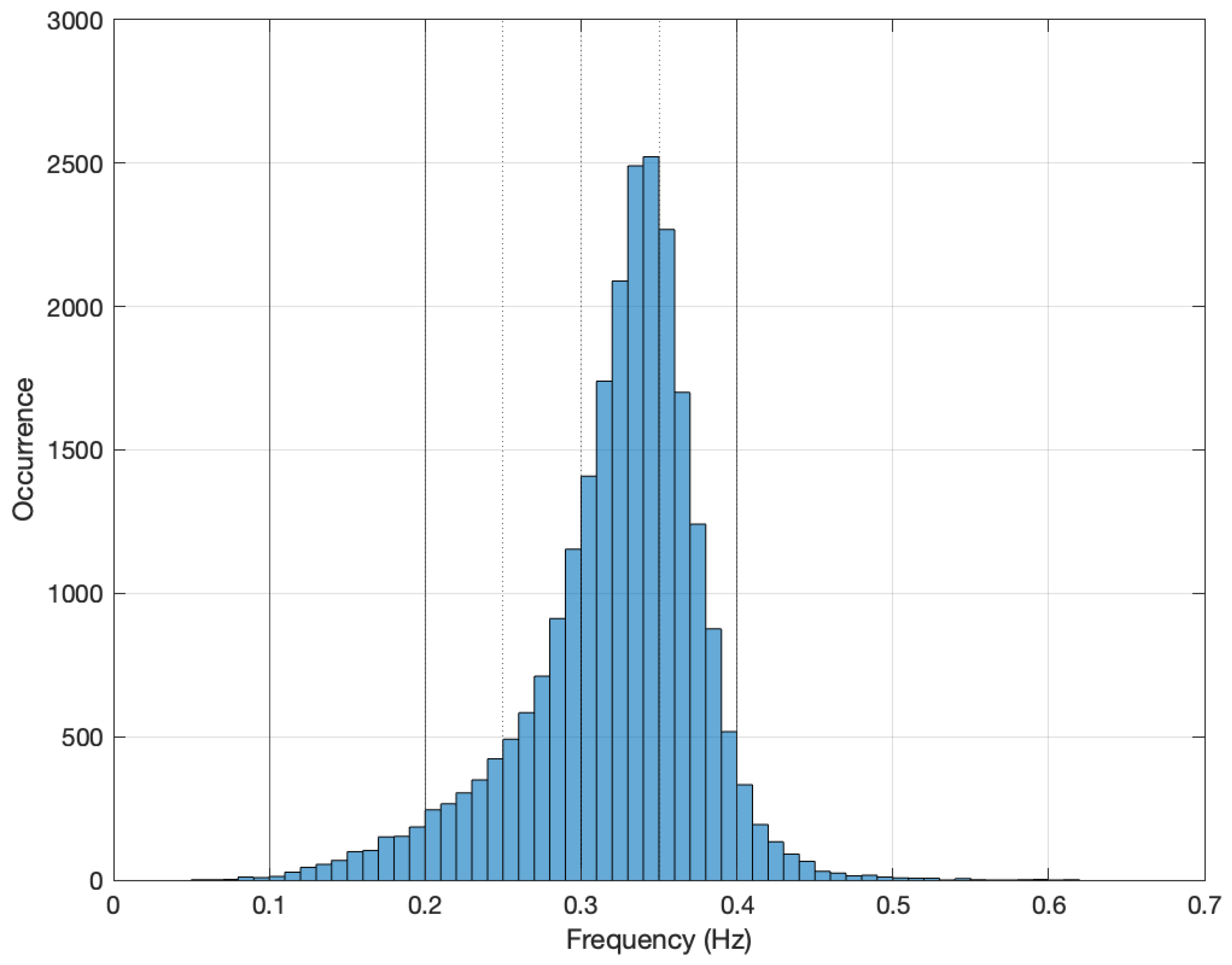
- The variation of the frequency of ocean waves are being scrutinized in depth.
- The implementation of complex neural network functionalities using integer, double and float type variables is studied in detail.
2. Related Works
2.1. Signal-Parameter Extraction
2.2. Embedded Time Series Applications
3. Materials and Methods
3.1. Background
3.2. Feature Extraction Procedure
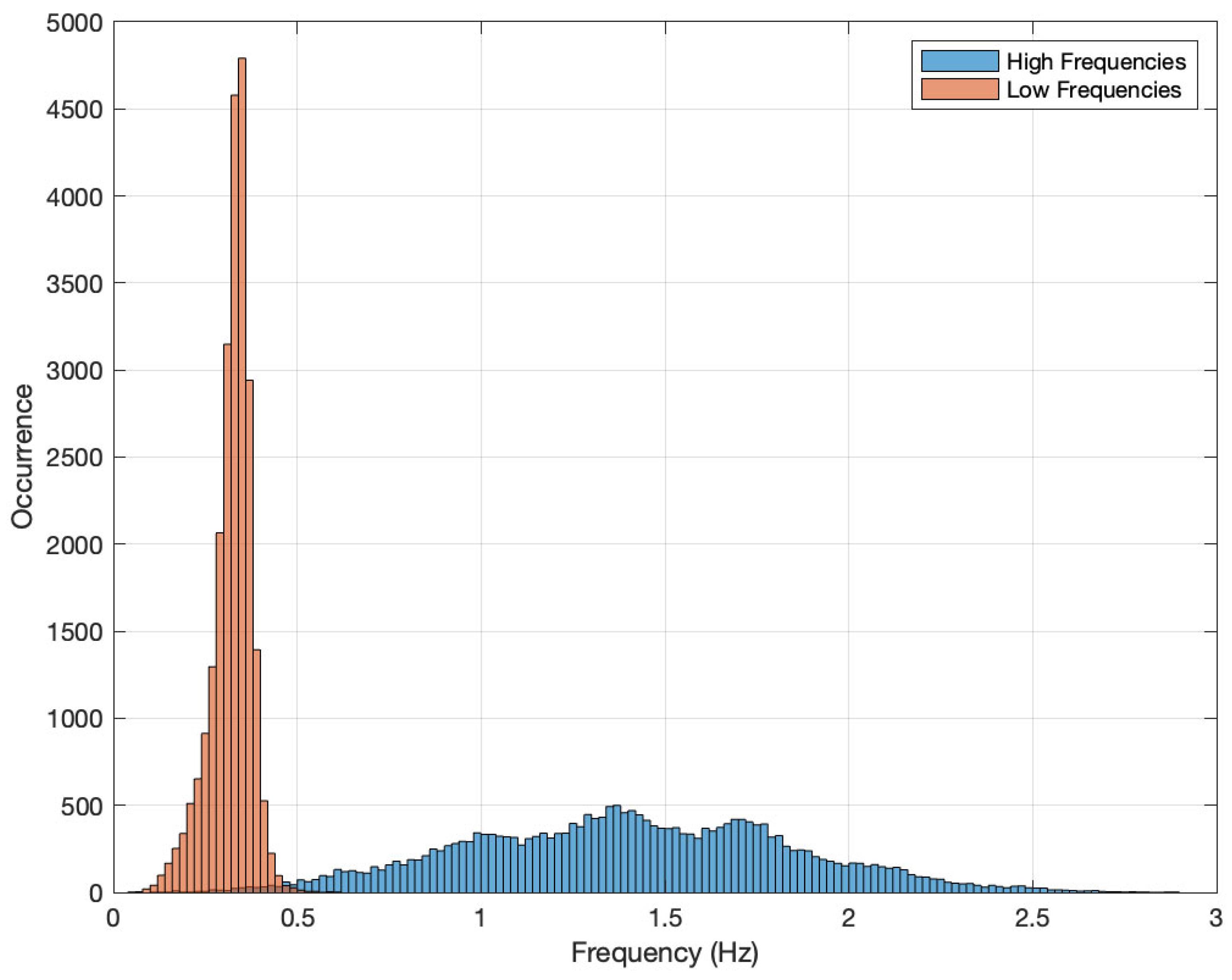
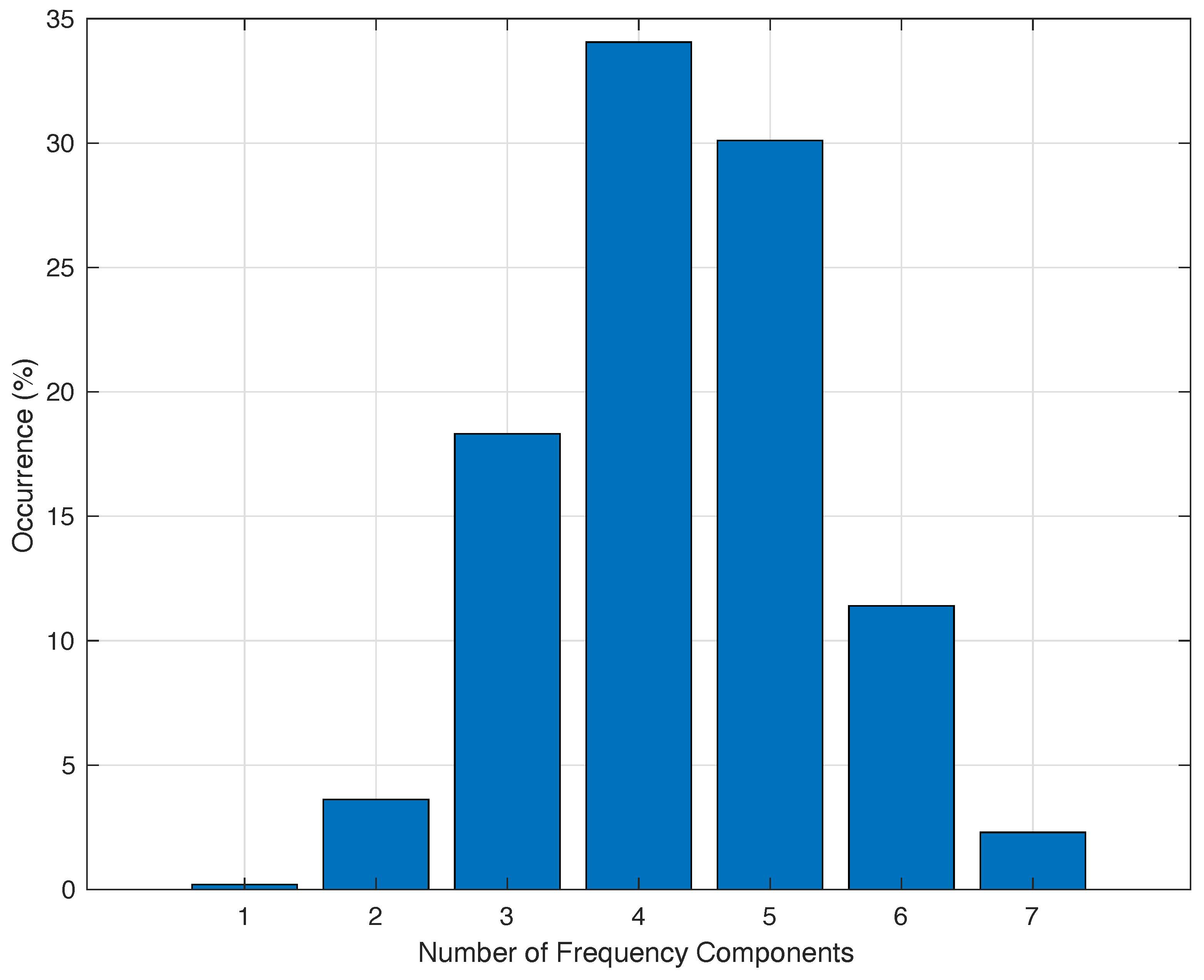
3.3. Involved Frequencies
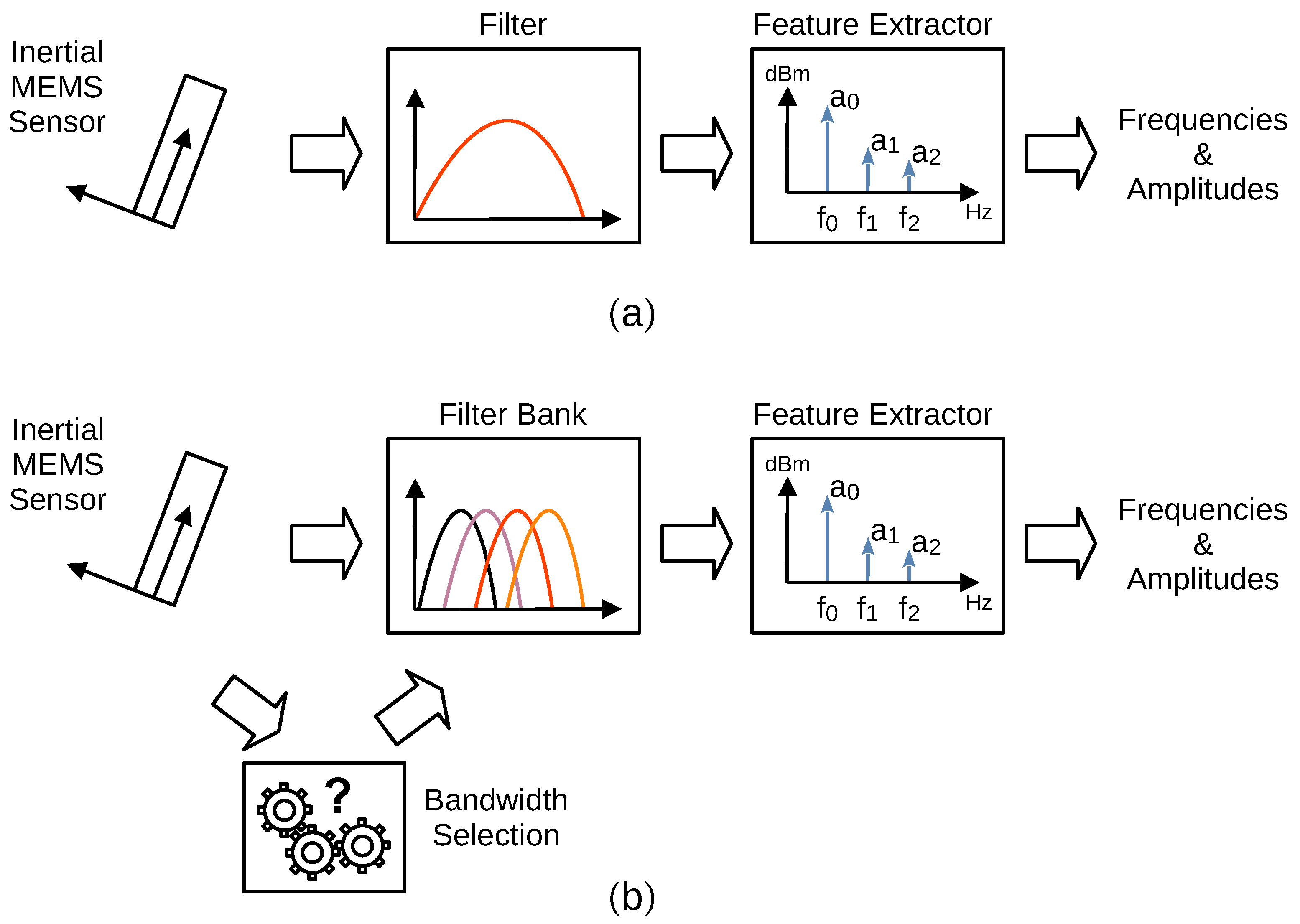
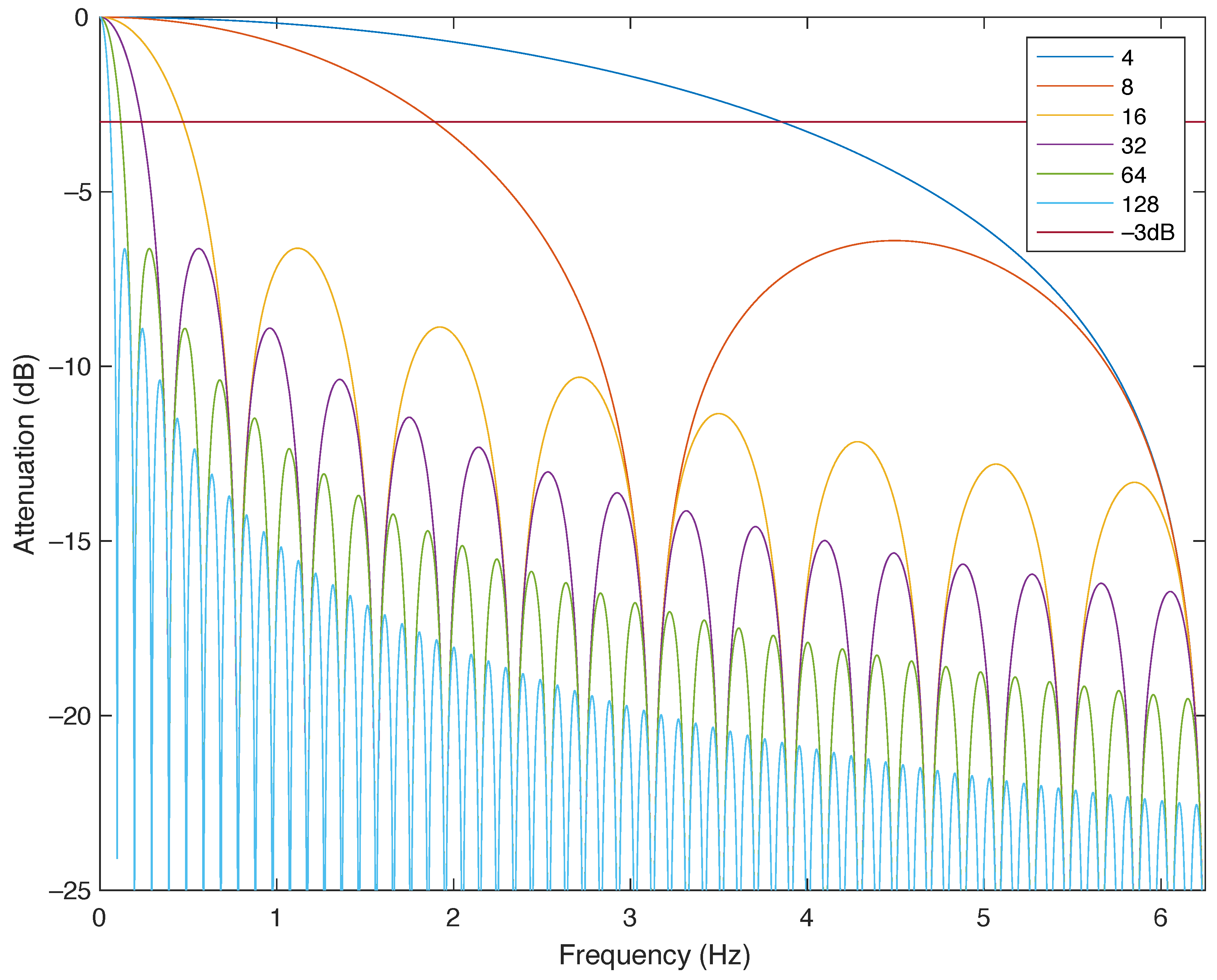
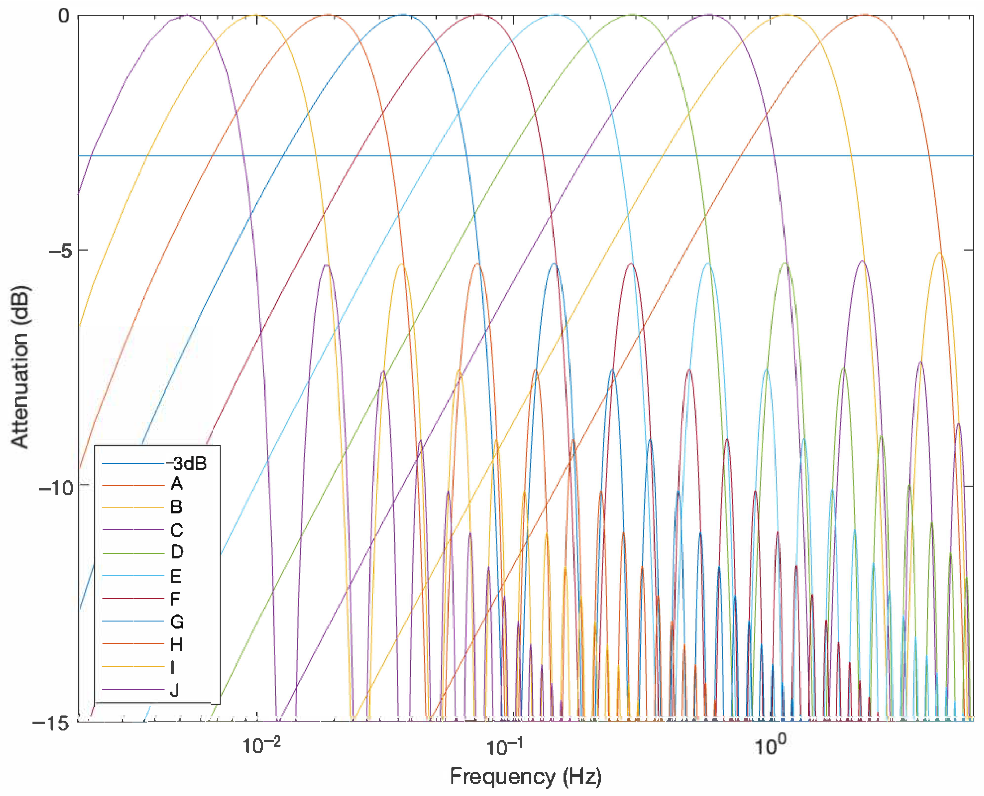
3.4. Filtering
3.5. AI-Based Solutions
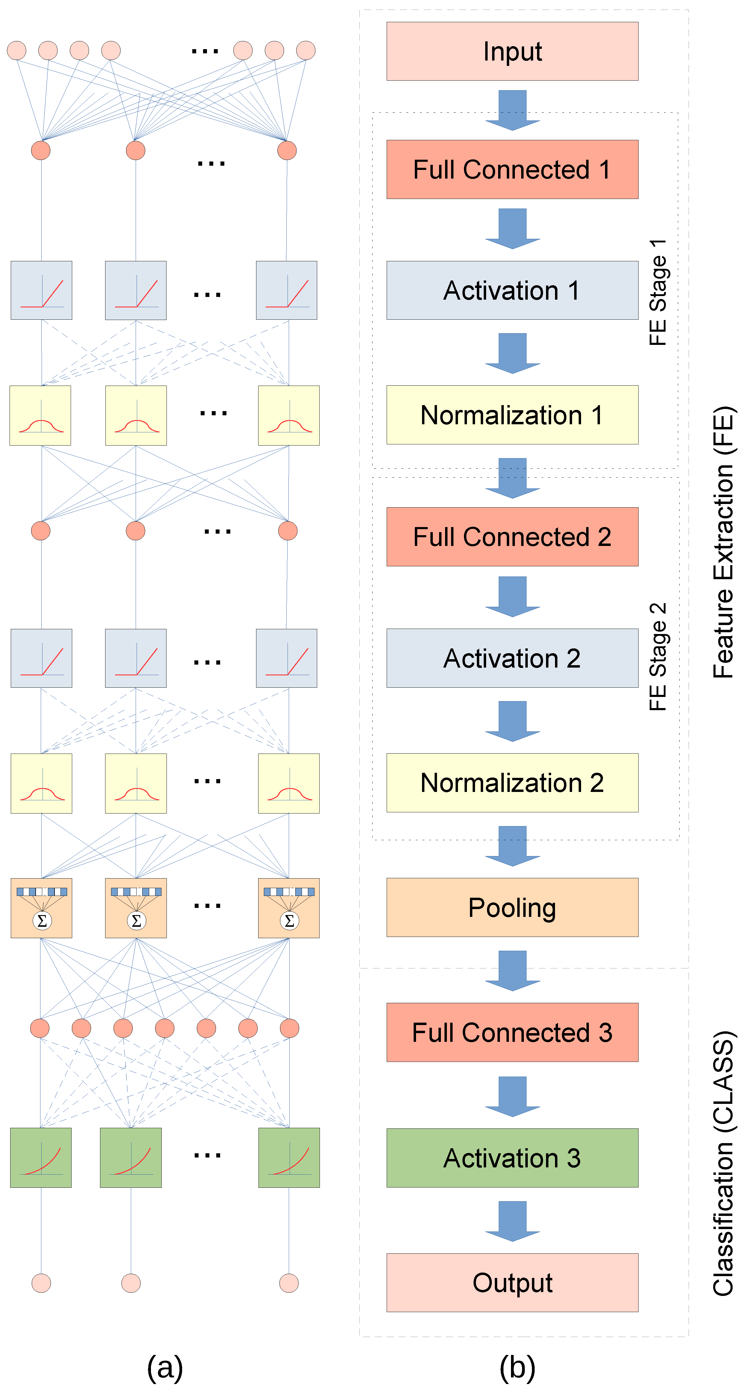
3.6. Deep Neural Network
4. Experiments and Discussion
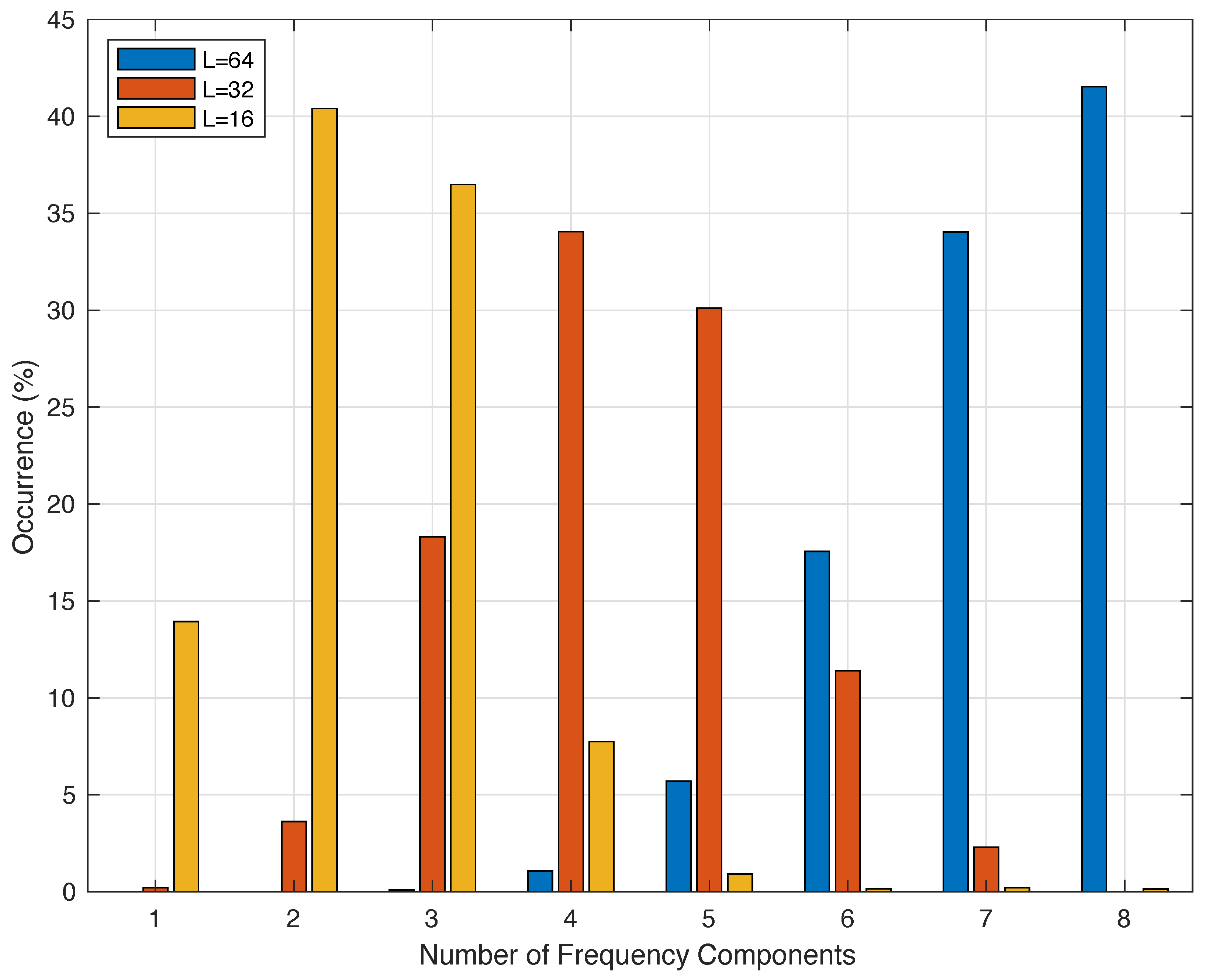
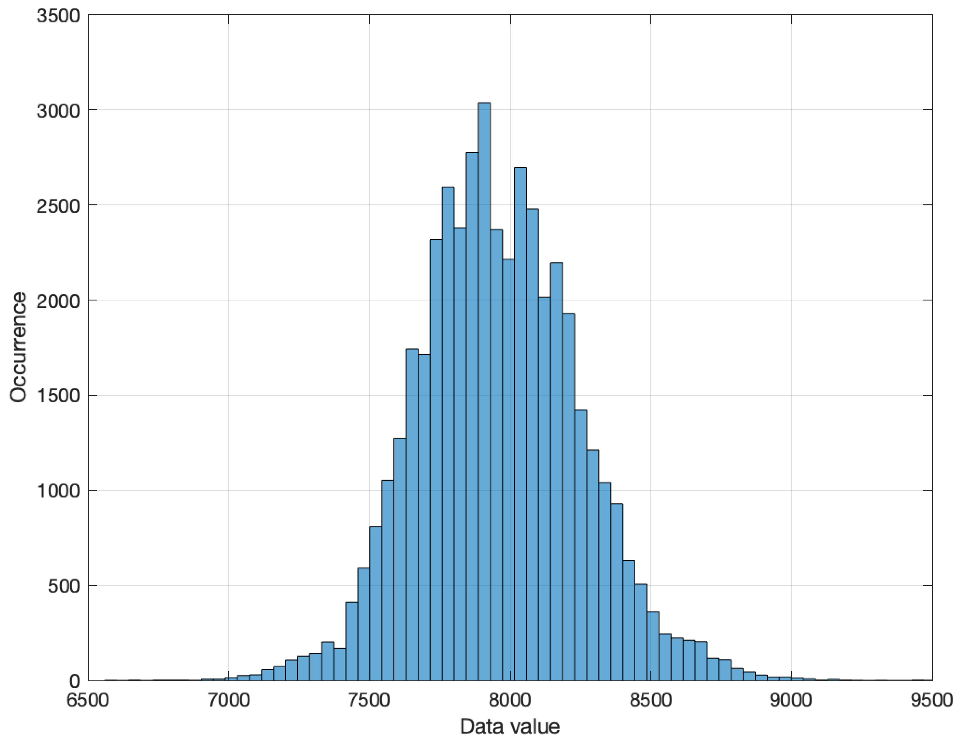
4.1. Training Data
4.2. Application Interface
4.2.1. Output
4.2.2. Inputs
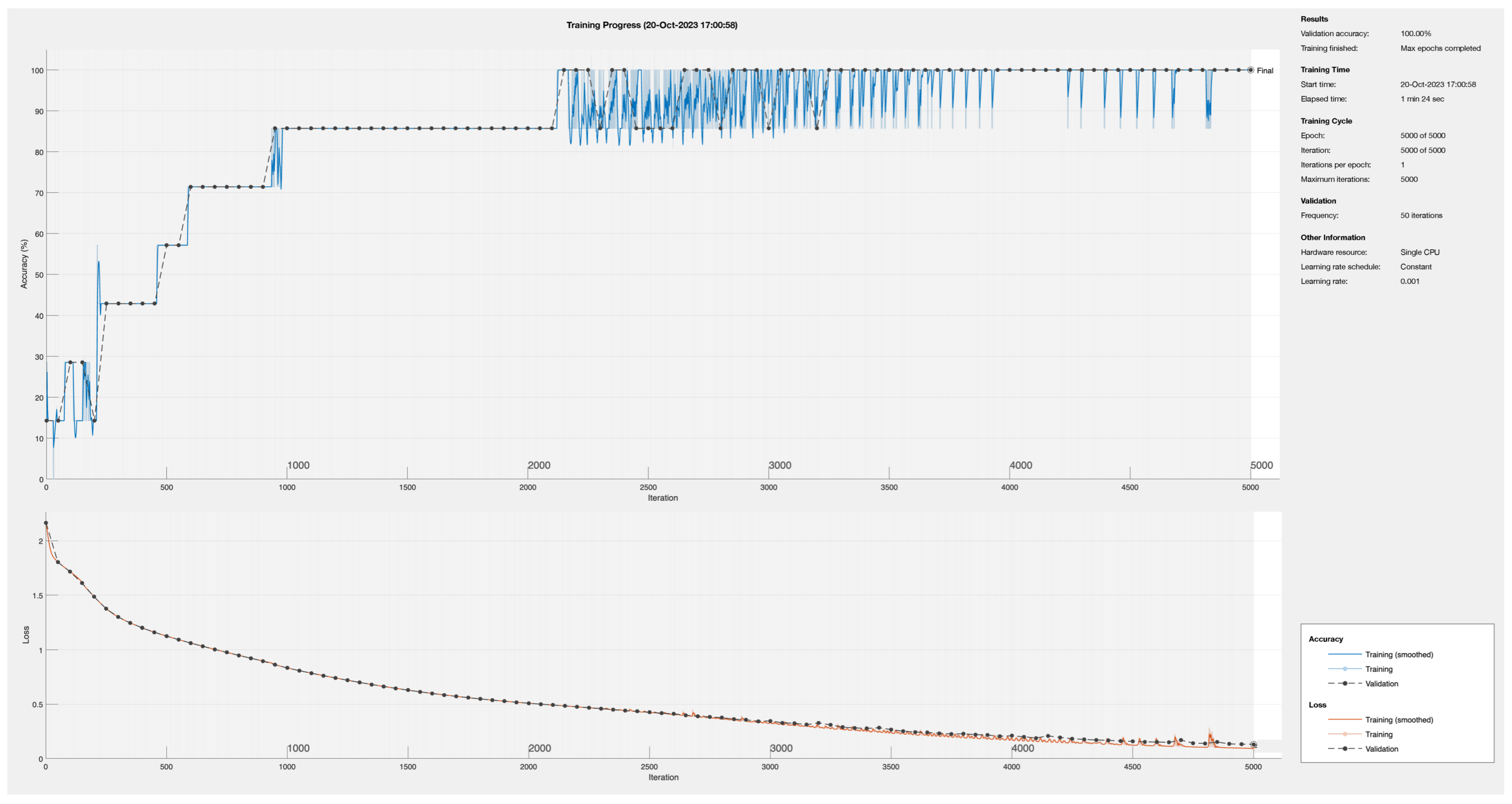
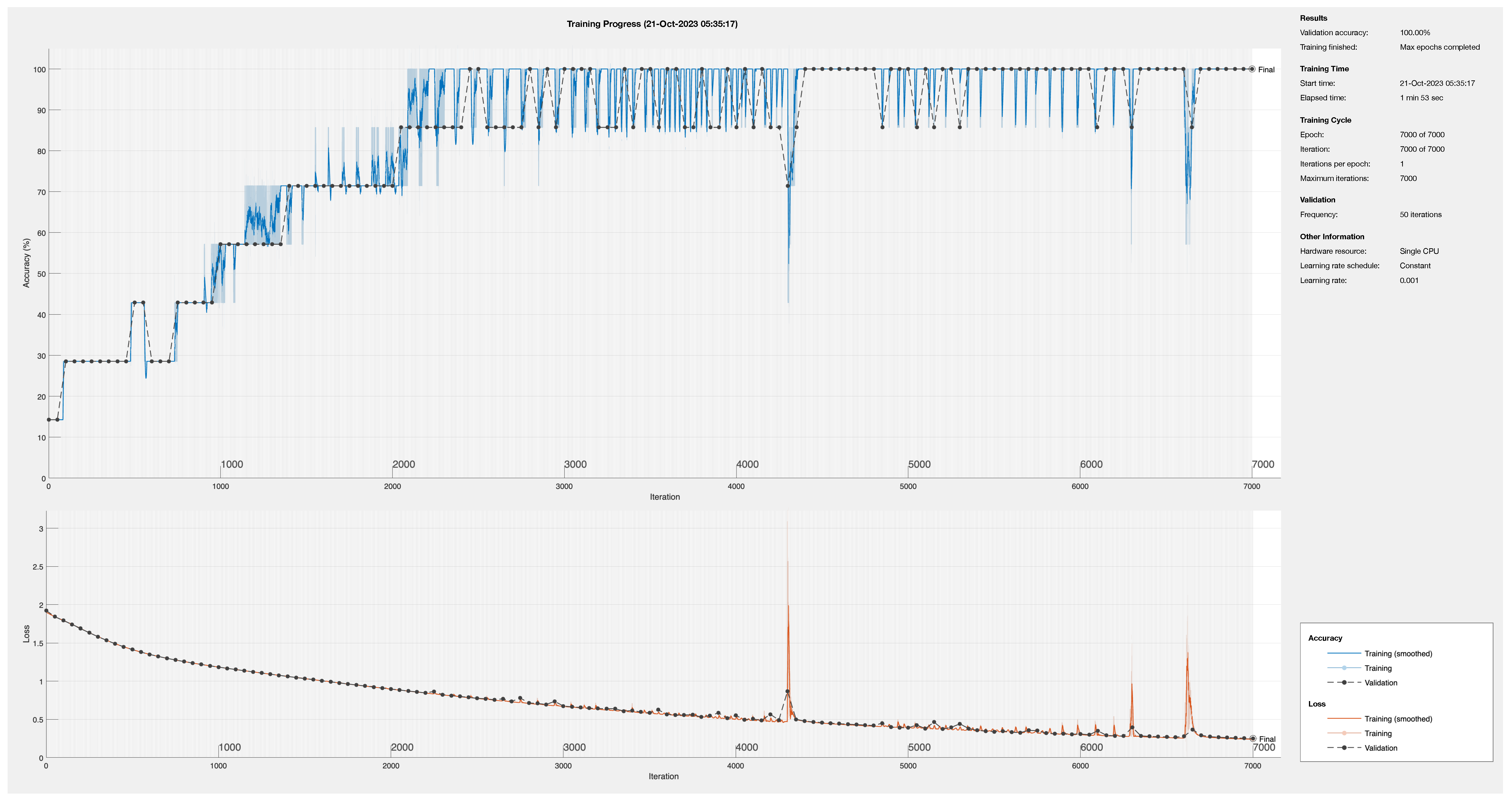
4.3. Training Process
Optimization
4.4. Practical Implementation
4.4.1. Input Layer
4.4.2. Fully Connected Layer
4.4.3. Activation Layer
4.4.4. Normalization Layer
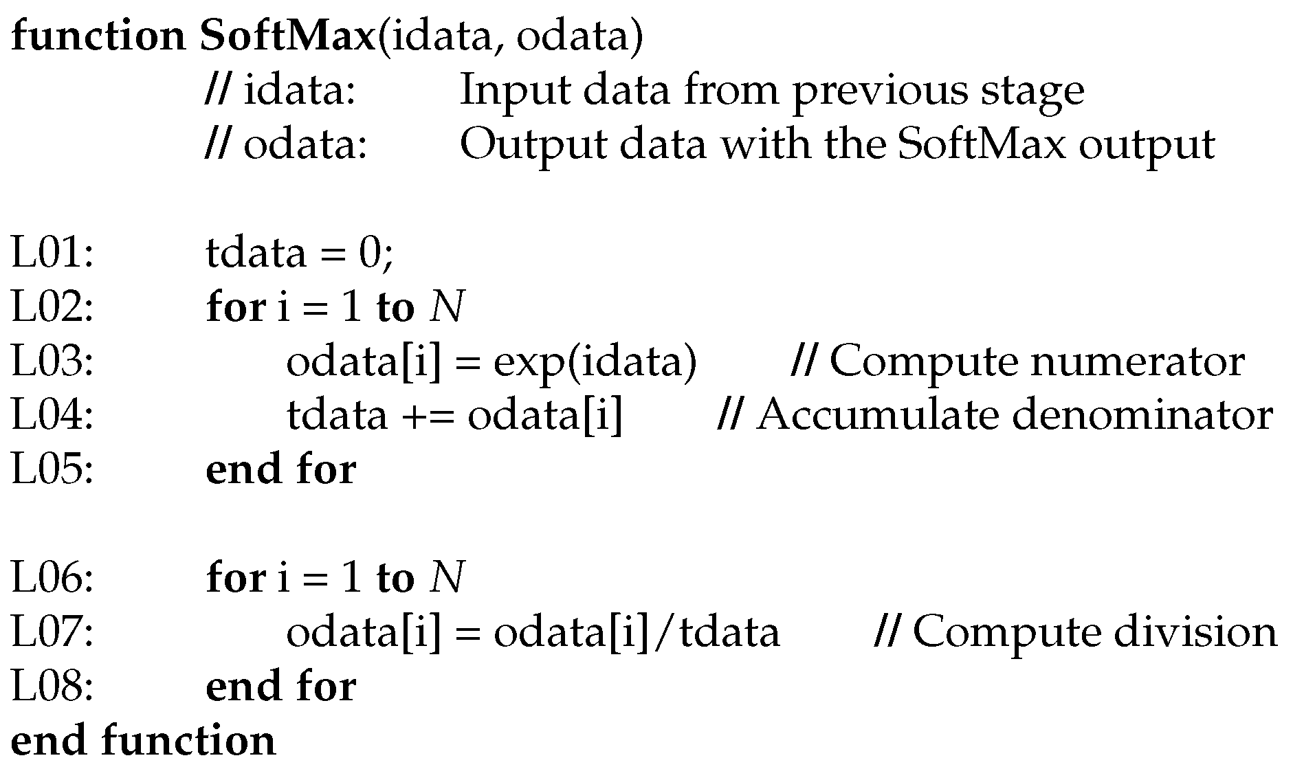
4.4.5. Activation Function
4.4.6. Complex Math Functions
4.5. Computational Effort Comparison
5. Conclusions
Author Contributions
Funding
Institutional Review Board Statement
Informed Consent Statement
Data Availability Statement
Conflicts of Interest
References
- Williams, A.J.; Heron, M.L.; Anderson, S.P. Technology of water flow measurement represented by thirty years of CMTC. In Proceedings of the OCEANS 2008, Quebec City, QC, Canada, 15–18 September 2008; pp. 1–8. [Google Scholar] [CrossRef]
- Chen, F.-W.; Liu, C.-W. Assessing the applicability of flow measurement by using non-contact observation methods in open channels. Environ. Monitor. Assess. 2020, 192, 289. [Google Scholar] [CrossRef]
- Haldar, B.; George, B.; Thirumurugan, K.; Muthiah, M.A.; Sudhakar, T.; Atmanand, M.A. Ocean Current Sensing Using Integrated Load Cell in the Mooring Line of a Data Buoy. IEEE Sens. J. 2024, 24, 858–865. [Google Scholar] [CrossRef]
- Hanel, R.; Marohn, L.; Wysujack, K.; Freese, M.; Pohlmann, J.-D.; Ohlmann, J.-D.; Waidmann, N.; Doring, R.; Warmerdam, W.; Scharrenburg, M.; et al. Research for PECH Committee—Environmental, Social and Economic Sustainability of European eel Management; European Union: Brussels, Belgium, 2019; Available online: https://op.europa.eu/en/publication-detail/-/publication/50cd51fa-358b-11e9-8d04-01aa75ed71a1/language-en (accessed on 10 February 2024).
- Crocioni, G.; Pau, D.; Delorme, J.-M.; Gruosso, G. Li-Ion Batteries Parameter Estimation with Tiny Neural Networks Embedded on Intelligent IoT Microcontrollers. IEEE Access 2020, 8, 122135–122146. [Google Scholar] [CrossRef]
- Montiel-Caminos, J.; Hernandez-Gonzalez, N.G.; Sosa, J.; Montiel-Nelson, J.A. Integer Arithmetic Algorithm for Fundamental Frequency Identification of Oceanic Currents. Sensors 2023, 23, 6549. [Google Scholar] [CrossRef] [PubMed]
- Shi, Y.; Yang, K.; Jiang, T.; Zhang, J.; Letaief, K.B. Communication-Efficient Edge AI: Algorithms and Systems. IEEE Commun. Surv. Tutor. 2020, 22, 2167–2191. [Google Scholar] [CrossRef]
- Barbuto, V.; Savaglio, C.; Chen, M.; Fortino, G. Disclosing Edge Intelligence: A Systematic Meta-Survey. Big Data Cogn. Comput. 2023, 7, 44. [Google Scholar] [CrossRef]
- Sun, J.; Aboutanios, E.; Smith, D.B. Low Cost and Precise Frequency Estimation in Unbalanced Three Phase Power Systems. IEEE Trans. Power Deliv. 2023, 38, 767–776. [Google Scholar] [CrossRef]
- Terriche, Y.; Laib, A.; Lashab, A.; Su, C.-L.; Guerrero, J.M.; Vasquez, J.C. A Frequency Independent Technique to Estimate Harmonics and Interharmonics in Shipboard Microgrids. IEEE Trans. Smart Grid 2022, 13, 888–899. [Google Scholar] [CrossRef]
- Nishad, A.; Upadhyay, A.; Pachori, R.B.; Acharya, U.R. Automated classification of hand movements using tunable-Q wavelet transform based filter-bank with surface electromyogram signals. Future Gener. Comput. Syst. 2019, 93, 96–110. [Google Scholar] [CrossRef]
- Zao, L.; Coelho, R. On the Estimation of Fundamental Frequency From Nonstationary Noisy Speech Signals Based on the Hilbert–Huang Transform. IEEE Signal Process. Lett. 2018, 25, 248–252. [Google Scholar] [CrossRef]
- Zhang, Z.; Yu, Q.; Zhang, Q.; Ning, N.; Li, J. A Kalman filtering based adaptive threshold algorithm for QRS complex detection. Biomed. Signal Process. Control 2020, 58, 101827. [Google Scholar] [CrossRef]
- Jwo, D.-J.; Biswal, A. Implementation and Performance Analysis of Kalman Filters with Consistency Validation. Mathematics 2023, 11, 521. [Google Scholar] [CrossRef]
- Marques, C.A.; Ribeiro, M.V.; Duque, C.A.; Ribeiro, P.F.; da Silva, E.A. A Controlled Filtering Method for Estimating Harmonics of Off-Nominal Frequencies. IEEE Trans. Smart Grid 2012, 3, 38–49. [Google Scholar] [CrossRef]
- Zhang, X.-M. Parameter Estimation of Shallow Wave Equation via cuckoo Search. Neural Comput. Appl. 2017, 28, 4047–4059. [Google Scholar] [CrossRef]
- Jiang, C.; Serrao, P.; Liu, M.; Cho, C. An Enhanced Genetic Algorithm for Parameter Estimation of Sinusoidal Signals. Appl. Sci. 2020, 10, 5110. [Google Scholar] [CrossRef]
- Anderson, R.; Sandsten, M. Time-frequency feature extraction for classification of episodic memory. EURASIP J. Adv. Signal Process. 2020, 2020, 19. [Google Scholar] [CrossRef]
- Li, X.; Zheng, J.; Li, M.; Ma, W.; Hu, Y. Frequency-Domain Fusing Convolutional Neural Network: A Unified Architecture Improving Effect of Domain Adaptation for Fault Diagnosis. Sensors 2021, 21, 450. [Google Scholar] [CrossRef]
- Yifan, W.; Kai, C.; Xuan, G.; Renjun, H.; Wenjian, Z.; Sheng, Y.; Gen, Q. A High-Precision and Wideband Fundamental Frequency Measurement Method for Synchronous Sampling Used in the Power Analyzer. Front. Energy Res. 2021, 9, 652386. [Google Scholar] [CrossRef]
- Queiroz, A.; Coelho, R. F0-Based Gammatone Filtering for Intelligibility Gain of Acoustic Noisy Signals. IEEE Signal Proc. Lett. 2021, 28, 1225–1229. [Google Scholar] [CrossRef]
- Queiroz, A.; Coelho, R. Noisy Speech Based Temporal Decomposition to Improve Fundamental Frequency Estimation. IEEE/ACM Trans. Audio Speech Lang. Process. 2022, 30, 2504–2513. [Google Scholar] [CrossRef]
- Castro-García, J.A.; Molina-Cantero, A.J.; Gómez-González, I.M.; Lafuente-Arroyo, S.; Merino-Monge, M. Towards Human Stress and Activity Recognition: A Review and a First Approach Based on Low-Cost Wearables. Electronics 2022, 11, 155. [Google Scholar] [CrossRef]
- Ao, S.-I.; Fayek, H. Continual Deep Learning for Time Series Modeling. Sensors 2023, 23, 7167. [Google Scholar] [CrossRef] [PubMed]
- Talib, M.A.; Majzoub, S.; Nasir, Q.; Jamal, D. A systematic literature review on hardware implementation of artificial intelligence algorithms. J. Supercomput. 2020, 77, 1897–1938. [Google Scholar] [CrossRef]
- NVIDIA. Jetson Platform. Available online: https://developer.nvidia.com/embedded-computing (accessed on 24 October 2023).
- Shin, D.-J.; Kim, J.-J. A Deep Learning Framework Performance Evaluation to Use YOLO in Nvidia Jetson Platform. Appl. Sci. 2022, 12, 3734. [Google Scholar] [CrossRef]
- Katsidimas, I.; Kostopoulos, V.; Kotzakolios, T.; Nikoletseas, S.E.; Panagiotou, S.H.; Tsakonas, C. An Impact Localization Solution Using Embedded Intelligence—Methodology and Experimental Verification via a Resource-Constrained IoT Device. Sensors 2023, 23, 896. [Google Scholar] [CrossRef] [PubMed]
- Zhou, S.; Du, Y.; Chen, B.; Li, Y.; Luan, X. An Intelligent IoT Sensing System for Rail Vehicle Running States Based on TinyML. IEEE Access 2022, 10, 98860–98871. [Google Scholar] [CrossRef]
- Kim, E.; Kim, J.; Park, J.; Ko, H.; Kyung, Y. TinyML-Based Classification in an ECG Monitoring Embedded System. Comput. Mater. Contin. 2023, 75, 1751. [Google Scholar] [CrossRef]
- Jordan, A.A.; Pegatoquet, A.; Castagnetti, A.; Raybaut, J.; Le Coz, P. Deep Learning for Eye Blink Detection Implemented at the Edge. IEEE Embed. Syst. Lett. 2021, 13, 130–133. [Google Scholar] [CrossRef]
- TinyML. Tiny Machine Learning at MIT. Available online: https://tinyml.mit.edu/ (accessed on 25 October 2023).
- TensorFlow. TensorFlow for Mobile and Edge. Available online: https://www.tensorflow.org/lite (accessed on 24 October 2023).
- stm32-cube-ai. Free Tool for Edge AI Developers. Available online: https://stm32ai.st.com/stm32-cube-ai/ (accessed on 25 October 2023).
- NanoEdgeAIStudio. Automated Machine Learning (ML) Tool for STM32 Developers. Available online: https://www.st.com/en/development-tools/nanoedgeaistudio.html (accessed on 25 October 2023).
- Sosa, J.; Montiel-Nelson, J.-A. Novel Deep-Water Tidal Meter for Offshore Aquaculture Infrastructures. Sensors 2022, 22, 5513. [Google Scholar] [CrossRef]
- Young, I.R. Regular, Irregular Waves and the Wave Spectrum. In Encyclopedia of Maritime and Offshore Engineering; John Wiley and Sons, Ltd.: Hoboken, NJ, USA, 2017; ISBN 978-1-118-47635-2. [Google Scholar]
- Ducrozet, G.; Bonnefoy, F.; Perignon, Y. Applicability and limitations of highly non-linear potential flow solvers in the context of water waves. Ocean Eng. 2017, 142, 233–244. [Google Scholar] [CrossRef]
- Lamb, H. Hydrodynamics, 6th ed.; Cambridge University Press: Cambridge, UK, 1932. [Google Scholar]
- Li, W.; Hacid, H.; Almazrouei, E.; Debbah, M. A Comprehensive Review and a Taxonomy of Edge Machine Learning: Requirements, Paradigms, and Techniques. AI 2023, 4, 729–786. [Google Scholar] [CrossRef]
- Moroz, L.; Samotyy, V.; Gepner, P.; Węgrzyn, M.; Nowakowski, G. Power Function Algorithms Implemented in Microcontrollers and FPGAs. Electronics 2023, 12, 3399. [Google Scholar] [CrossRef]


| Reference | Year | Functions | Language | Domain | Input Filter | Equipment |
|---|---|---|---|---|---|---|
| [15] | 2012 | FIR, sin, sqrt | - | Fixed | Desktop PC | |
| [16] | 2017 | GA | C | Fixed | Desktop PC | |
| [12] | 2018 | Hilbert | Matlab | Fixed | Desktop PC | |
| [11] | 2019 | Wavelet, log | Matlab | Filter Bank | Desktop PC | |
| [17] | 2020 | GA | - | Fixed | Desktop PC | |
| [13] | 2020 | Kal | Matlab | Fixed | FPGA, Cortex-M4 * | |
| [20] | 2021 | FFT, GA, sqrt | C | Fixed | FPGA, Desktop PC | |
| [21] | 2021 | Hilbert | Matlab | Filter Bank | Desktop PC | |
| [10] | 2022 | FFT | Matlab | Fixed | Desktop PC | |
| [22] | 2022 | Hilbert | Matlab | Filter Bank | Desktop PC | |
| [9] | 2023 | FFT, IFFT, sin, sqrt | Matlab | Fixed | Desktop PC | |
| [14] | 2023 | Kal, sqrt, covariance | Matlab | Fixed | Desktop PC | |
| [6] | 2023 | FIR | C | Fixed | Cortex-M0 |
| Filter | −3 dB | −0.58 dB | ||||
|---|---|---|---|---|---|---|
| ID | Length | Period | ||||
| (Samples) | (s) | (Hz) | (Hz) | (Hz) | (Hz) | |
| A | 4 | 0.64 | 4.191 | 0.782 | 3.178 | 1.573 |
| B | 8 | 1.28 | 2.083 | 0.391 | 1.573 | 0.788 |
| C | 16 | 2.56 | 1.044 | 0.189 | 0.788 | 0.394 |
| D | 32 | 5.12 | 0.521 | 0.099 | 0.394 | 0.197 |
| E | 64 | 10.24 | 0.262 | 0.048 | 0.197 | 0.098 |
| F | 128 | 20.48 | 0.130 | 0.024 | 0.098 | 0.049 |
| G | 256 | 40.96 | 0.066 | 0.012 | 0.049 | 0.025 |
| H | 512 | 81.92 | 0.033 | 0.007 | 0.025 | 0.013 |
| I | 1024 | 163.84 | 0.017 | 0.004 | 0.013 | 0.007 |
| J | 2048 | 327.68 | 0.008 | 0.002 | 0.007 | 0.004 |
| Math | Double | Float | Int32 | Int16 | ||||||||
|---|---|---|---|---|---|---|---|---|---|---|---|---|
| Function | Min | Avg | Max | Min | Avg | Max | Min | Avg | Max | Min | Avg | Max |
| 7241 | 7400 | 7555 | 7335 | 7494 | 7649 | 7399 | 7556 | 7713 | 7398 | 7555 | 7712 | |
| 6673 | 6873 | 7242 | 6770 | 6951 | 7339 | 6800 | 6980 | 7362 | 6796 | 6976 | 7358 | |
| 1373 | 1427 | 1485 | 281 | 282 | 293 | 127 | 136 | 152 | 125 | 134 | 150 | |
| Math | Double | Float | Int32 | Int16 | ||||||||
|---|---|---|---|---|---|---|---|---|---|---|---|---|
| Function | Min | Avg | Max | Min | Avg | Max | Min | Avg | Max | Min | Avg | Max |
| 5282 | 5394 | 5282 | 5371 | 5482 | 5598 | 5404 | 5515 | 5633 | 5412 | 5525 | 5636 | |
| 4612 | 4732 | 5014 | 5092 | 4810 | 4689 | 4711 | 4830 | 4711 | 4710 | 4832 | 4711 | |
| 903 | 937 | 903 | 196 | 197 | 202 | 84 | 89 | 99 | 84 | 89 | 99 | |
| Layer | Elements | Integer-Double | Integer-Float | ||
|---|---|---|---|---|---|
| Name | (Neurons) | Cycles * | Operation | Cycles * | Operation |
| Input | 32 | 0 | Integer | 0 | Integer |
| Full Connected 1 | 5 | 966 | Integer | 966 | Integer |
| Activation 1 | 5 | 70 | Integer | 70 | Integer |
| Normalization 1 | 5 | 2883 | Double | 1232 | Float |
| Full Connected 2 | 5 | 3276 | Double | 1942 | Float |
| Activation 2 | 5 | 418 | Double | 331 | Float |
| Normalization 2 | 5 | 2884 | Double | 1232 | Float |
| Pooling | 7 | 0 | Double | 0 | Float |
| Full Connected 3 | 7 | 4008 | Double | 4008 | Float |
| Activation 3 | 7 | 61,792 | Double | 53,920 | Float |
| Outputs | 7 | 0 | Integer | 0 | Integer |
| Total Cycles | 76,297 | 63,701 | |||
| Time @ 8 MHz | |||||
| Layer | Elements | Integer-Double | Integer-Float | ||
|---|---|---|---|---|---|
| Name | (Neurons) | Cycles * | Operation | Cycles * | Operation |
| Input | 32 | 0 | Integer | 0 | Integer |
| Full Connected 2 | 3 | 562 | Integer | 562 | Integer |
| Activation 2 | 3 | 24 | Integer | 24 | Integer |
| Normalization 2 | 3 | 1725 | Double | 736 | Float |
| Pooling | 7 | 0 | Double | 0 | Float |
| Full Connected 3 | 7 | 4008 | Double | 4008 | Float |
| Activation 3 | 7 | 61,792 | Double | 53,920 | Float |
| Output | 7 | 0 | Integer | 0 | Integer |
| Total Cycles | 68,111 | 59,250 | |||
| Time @ 8 MHz | |||||
Disclaimer/Publisher’s Note: The statements, opinions and data contained in all publications are solely those of the individual author(s) and contributor(s) and not of MDPI and/or the editor(s). MDPI and/or the editor(s) disclaim responsibility for any injury to people or property resulting from any ideas, methods, instructions or products referred to in the content. |
© 2024 by the authors. Licensee MDPI, Basel, Switzerland. This article is an open access article distributed under the terms and conditions of the Creative Commons Attribution (CC BY) license (https://creativecommons.org/licenses/by/4.0/).
Share and Cite
Hernandez-Gonzalez, N.G.; Montiel-Caminos, J.; Sosa, J.; Montiel-Nelson, J.A. An Edge Computing Application of Fundamental Frequency Extraction for Ocean Currents and Waves. Sensors 2024, 24, 1358. https://doi.org/10.3390/s24051358
Hernandez-Gonzalez NG, Montiel-Caminos J, Sosa J, Montiel-Nelson JA. An Edge Computing Application of Fundamental Frequency Extraction for Ocean Currents and Waves. Sensors. 2024; 24(5):1358. https://doi.org/10.3390/s24051358
Chicago/Turabian StyleHernandez-Gonzalez, Nieves G., Juan Montiel-Caminos, Javier Sosa, and Juan A. Montiel-Nelson. 2024. "An Edge Computing Application of Fundamental Frequency Extraction for Ocean Currents and Waves" Sensors 24, no. 5: 1358. https://doi.org/10.3390/s24051358
APA StyleHernandez-Gonzalez, N. G., Montiel-Caminos, J., Sosa, J., & Montiel-Nelson, J. A. (2024). An Edge Computing Application of Fundamental Frequency Extraction for Ocean Currents and Waves. Sensors, 24(5), 1358. https://doi.org/10.3390/s24051358