Author Contributions
Conceptualizations, D.R., J.S., N.A., B.B. and F.G.; methodology, D.R., J.S., N.A., B.B. and F.G.; software, D.R., J.S. and N.A.; validation, J.S.; formal analysis, D.R. and N.A.; investigation, D.R., J.S., N.A. and B.B.; resources, B.B. and F.G.; data curation, J.S. and B.B.; writing—original draft preparation, D.R. and N.A.; writing—review and editing, J.S., A.D., J.B., K.R., B.B., S.A.R. and F.G.; visualisation, D.R., J.S., N.A. and B.B.; supervision, B.B. and F.G.; project administration, B.B. and F.G.; funding acquisition, B.B., J.B., S.A.R. and F.G. All authors have read and agreed to the published version of the manuscript.
Figure 1.
Processing pipeline of data preparation for classification of health status of moss and lichen in Antarctic environment.
Figure 1.
Processing pipeline of data preparation for classification of health status of moss and lichen in Antarctic environment.
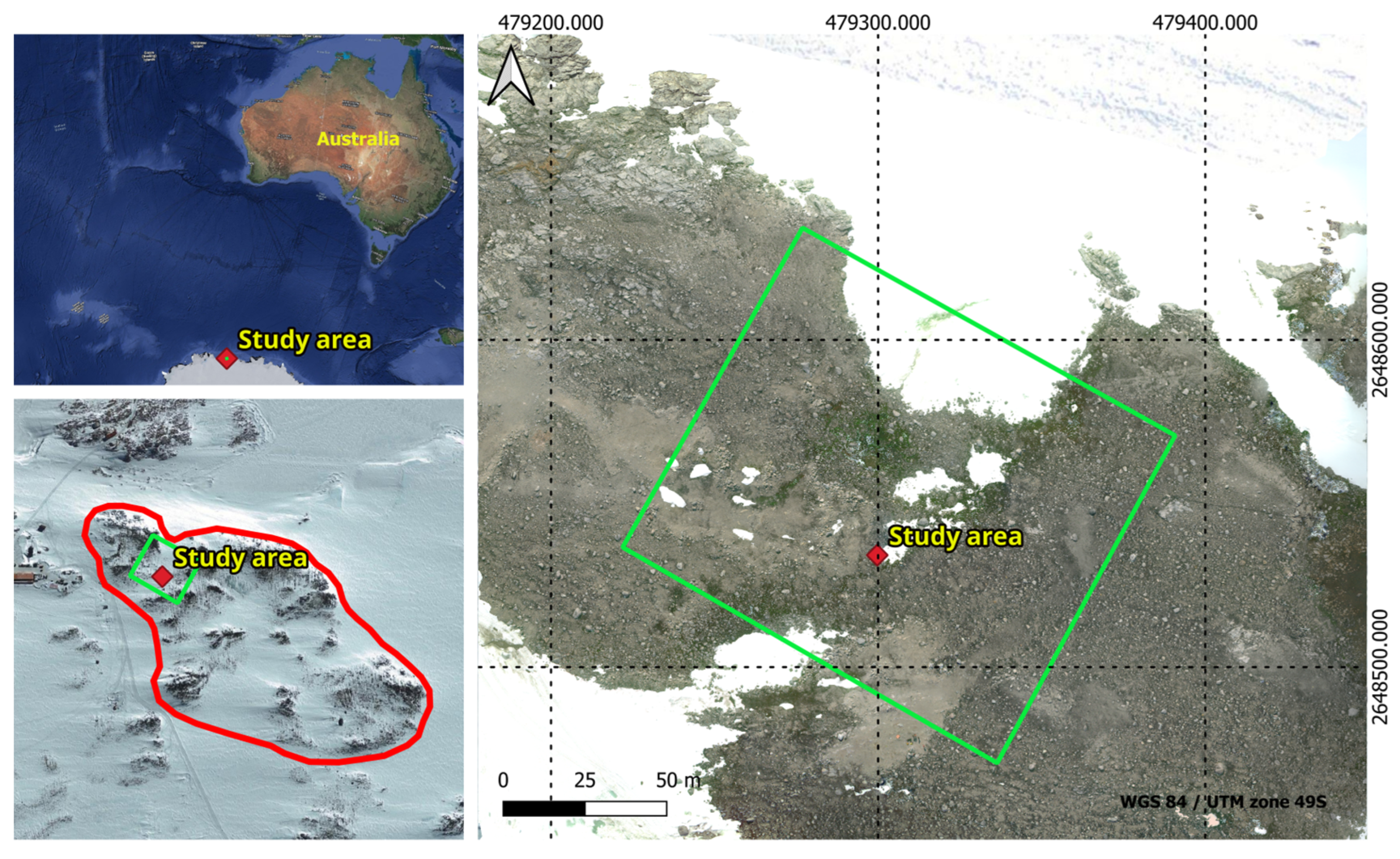
Figure 2.
Geographical representation of ASPA 135 outlined by the red polygon, and the study area delineated by the green polygon on the map.
Figure 2.
Geographical representation of ASPA 135 outlined by the red polygon, and the study area delineated by the green polygon on the map.
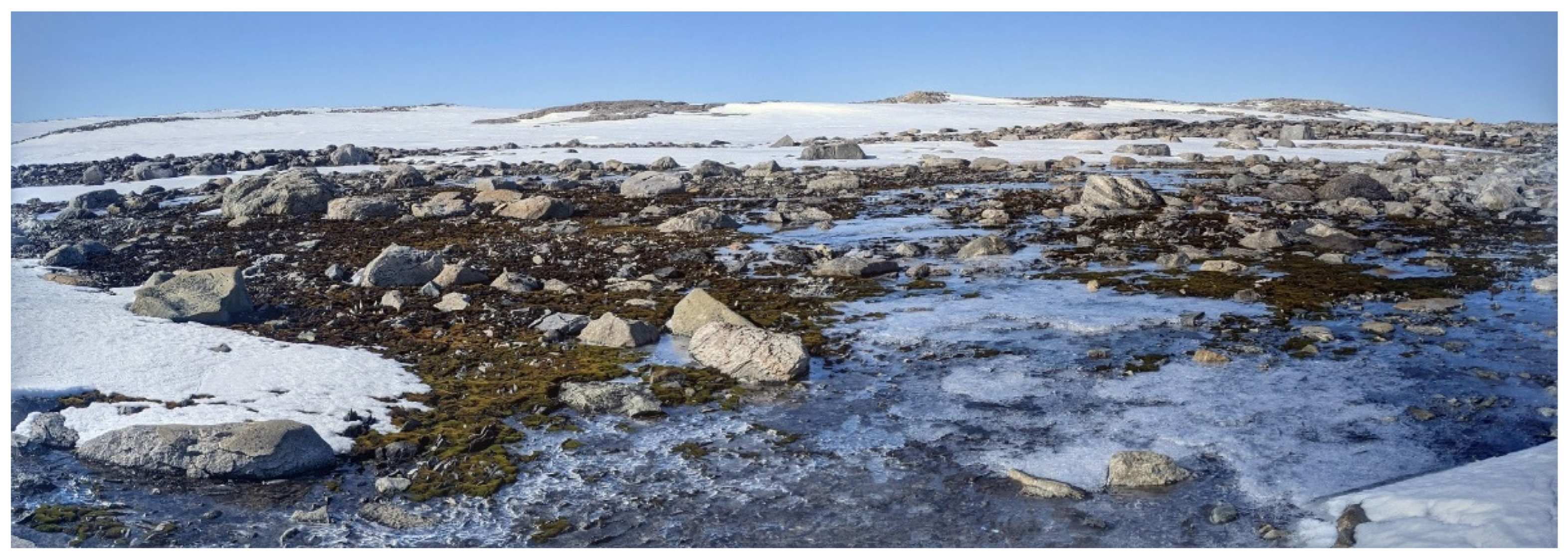
Figure 3.
Ground image of study area depicting distribution of moss and lichen vegetation.
Figure 3.
Ground image of study area depicting distribution of moss and lichen vegetation.
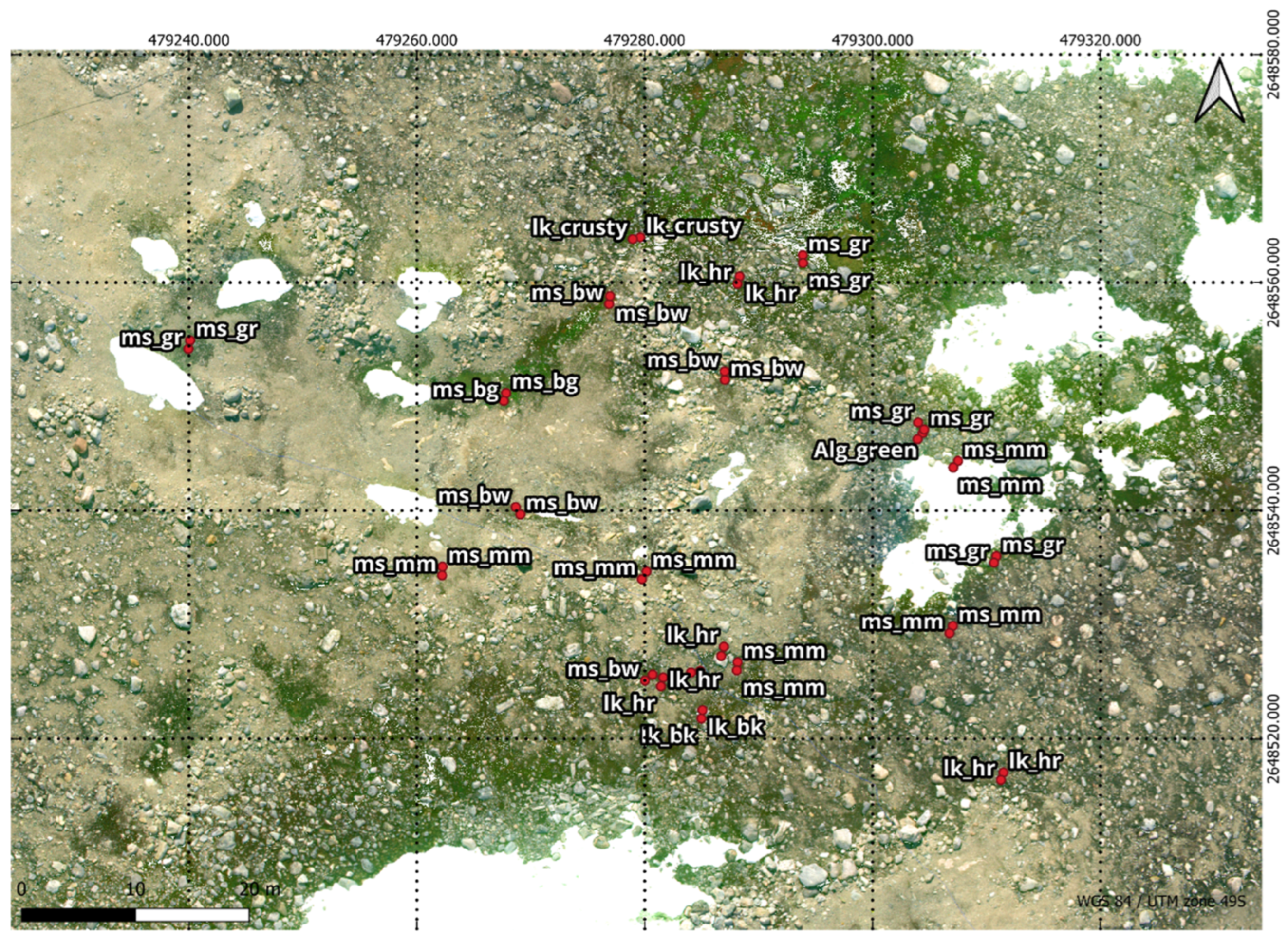
Figure 4.
Ground truth points overlaid on RGB Orthomosaic: Healthy moss, characterised by a green colour, is labelled as ms_gr & ms_bg. Stressed moss, displaying shades of orange or red, is denoted as ms_rd. Moribund moss, with brown or black hues, is identified by the labels ms_bw & ms_mm. Featured lichen, include those with “hairy” (fructicose Usnea spp.) black, and crusty (crustose) attributes, were classified using the labels lk_hr & lk_bk & lk_crusty.
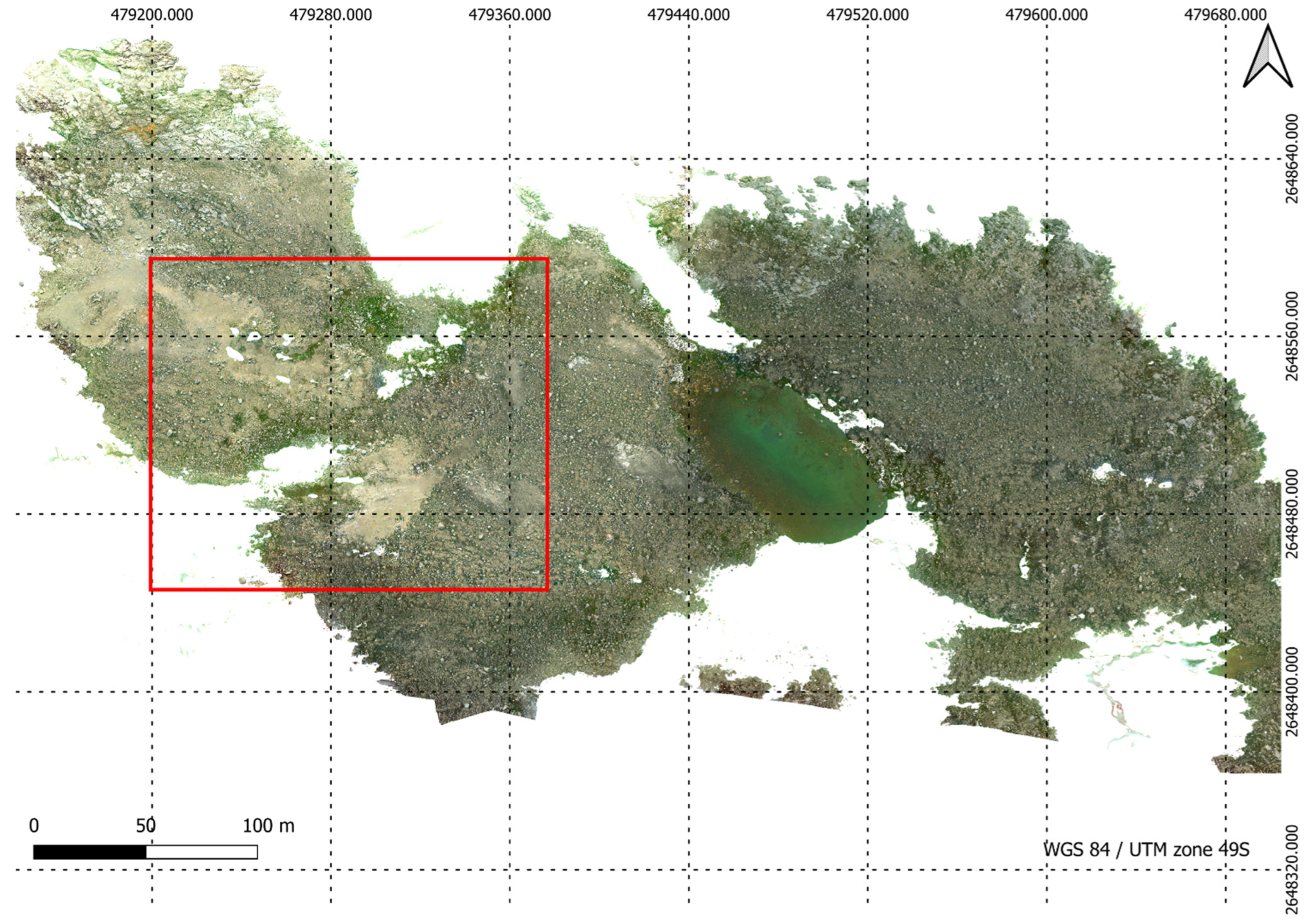
Figure 5.
High resolution RGB orthomosaic of ASPA 135 developed from Sony Alpha 5100 raw images.
Figure 5.
High resolution RGB orthomosaic of ASPA 135 developed from Sony Alpha 5100 raw images.
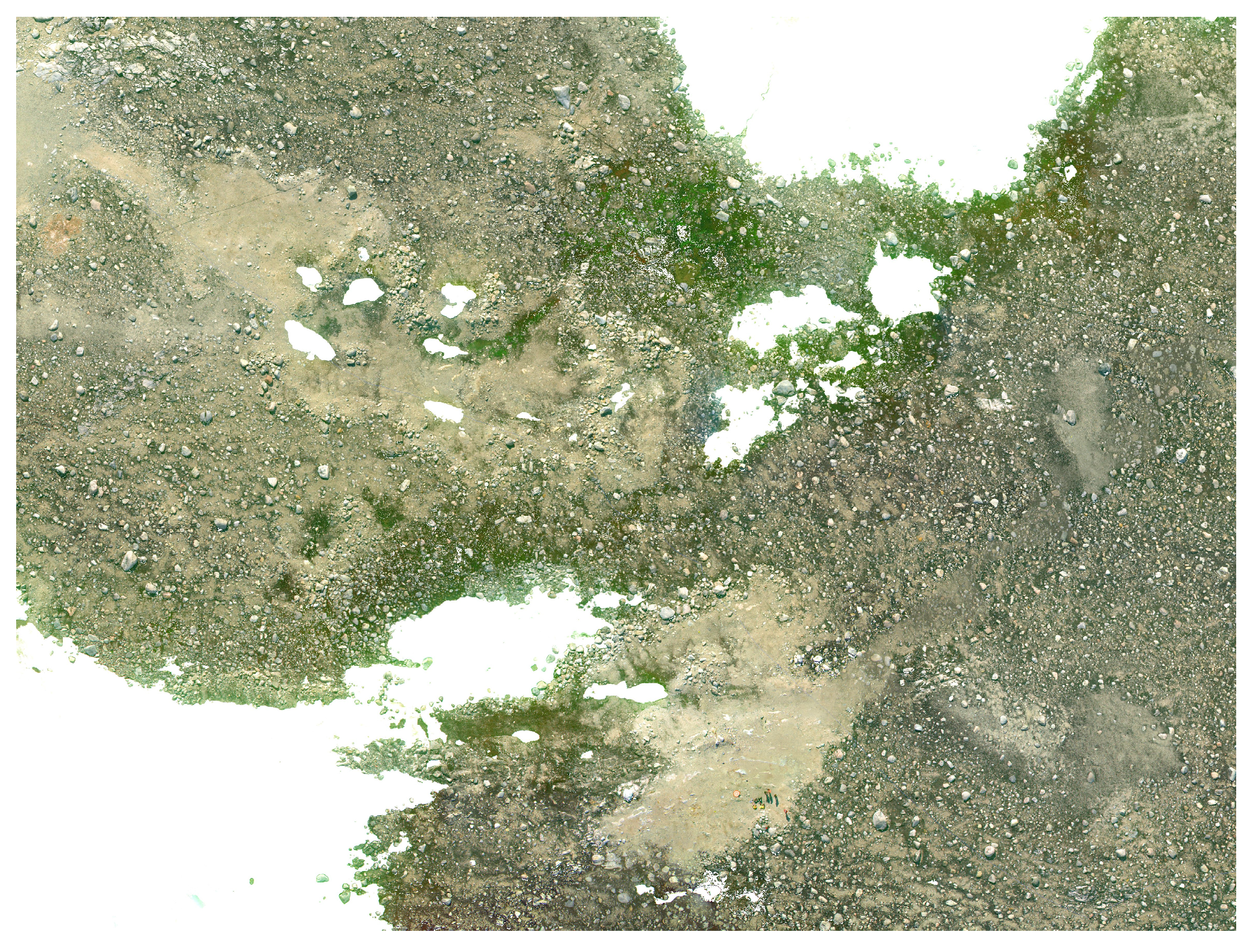
Figure 6.
A region of high resolution RGB orthomosaic.
Figure 6.
A region of high resolution RGB orthomosaic.
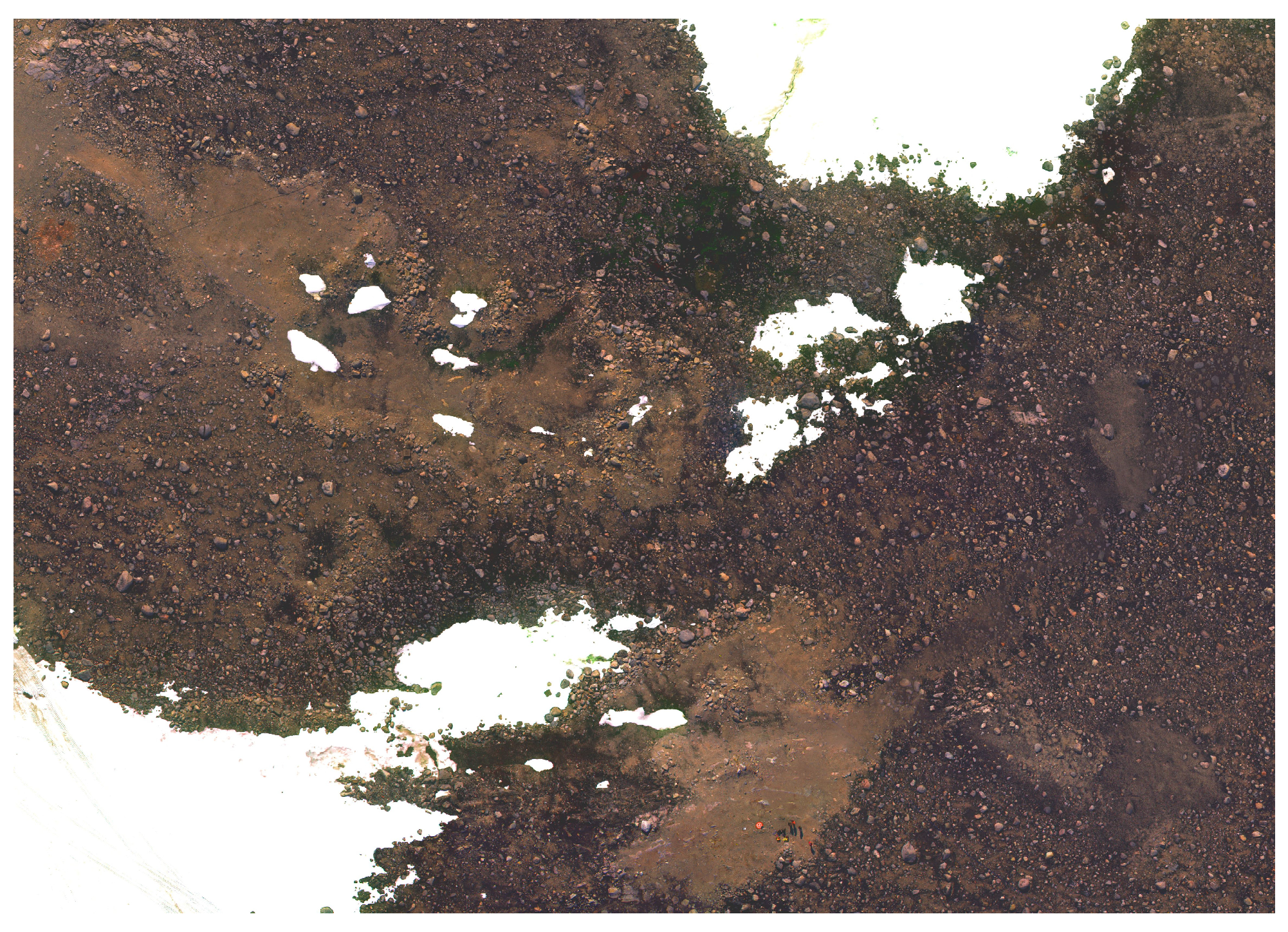
Figure 7.
A region of high resolution multispectral orthomosaic.
Figure 7.
A region of high resolution multispectral orthomosaic.
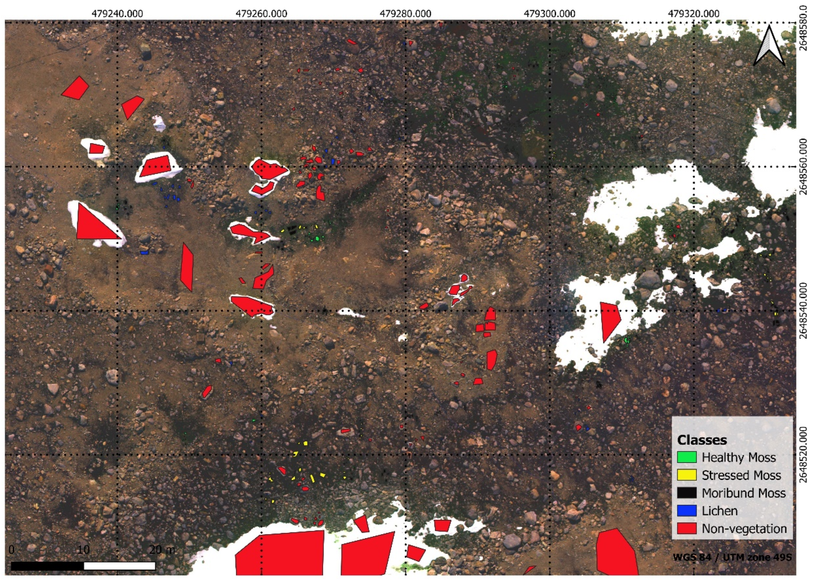
Figure 8.
Labelled polygons with different classes over georeferenced multispectral orthomosaic.
Figure 8.
Labelled polygons with different classes over georeferenced multispectral orthomosaic.
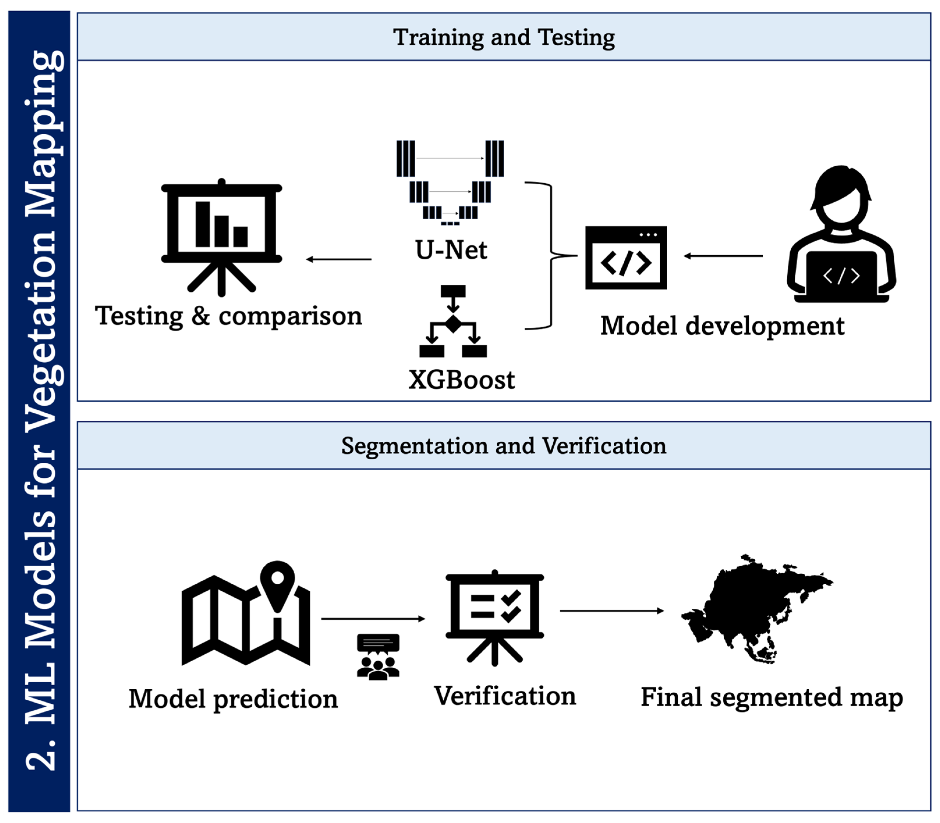
Figure 9.
Processing pipeline of machine learning for classification of health status of moss and lichen in an Antarctic environment.
Figure 9.
Processing pipeline of machine learning for classification of health status of moss and lichen in an Antarctic environment.
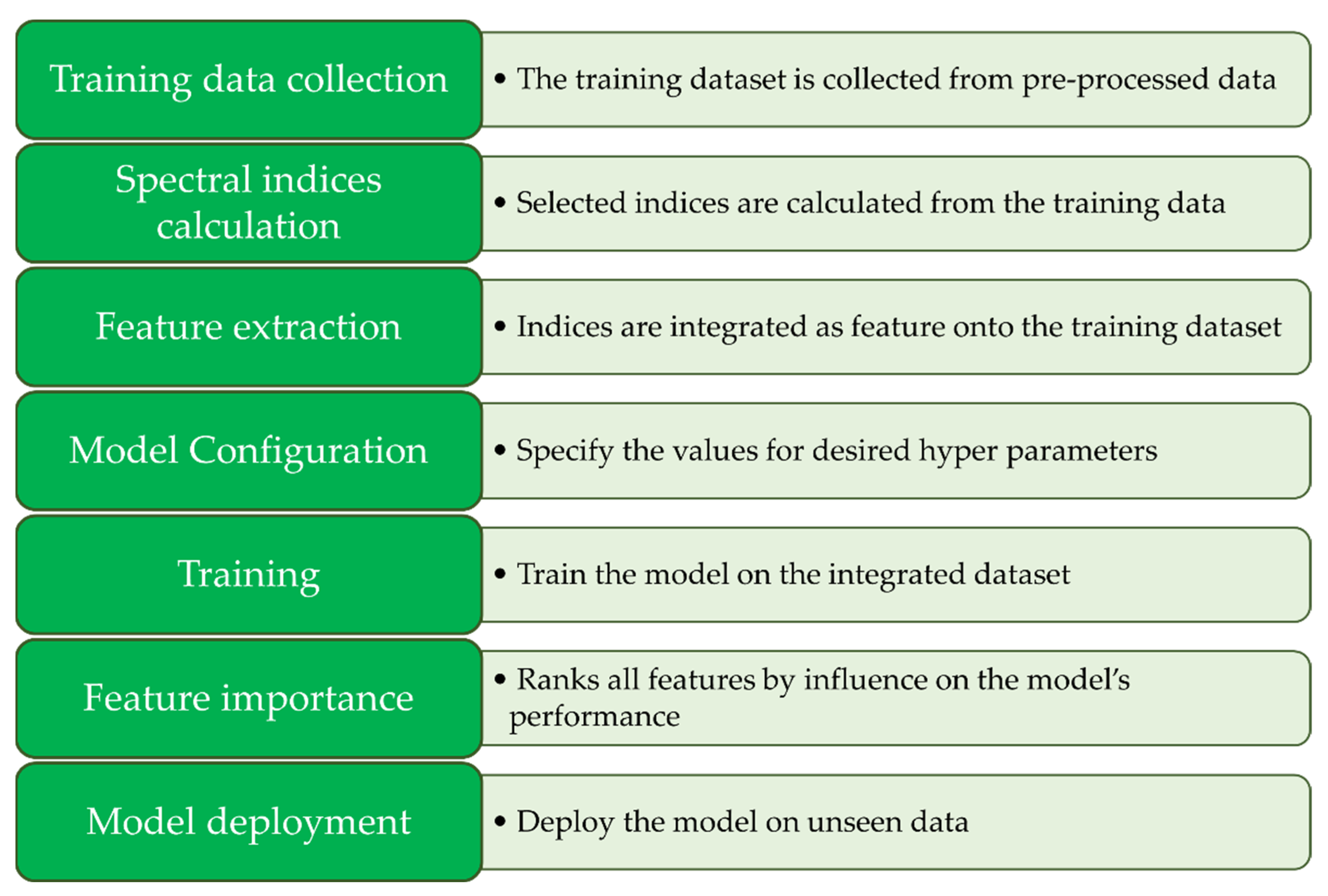
Figure 10.
Processing pipeline employed for XGBoost segmentation, showcasing the sequential steps and pivotal components involved in the methodology.
Figure 10.
Processing pipeline employed for XGBoost segmentation, showcasing the sequential steps and pivotal components involved in the methodology.
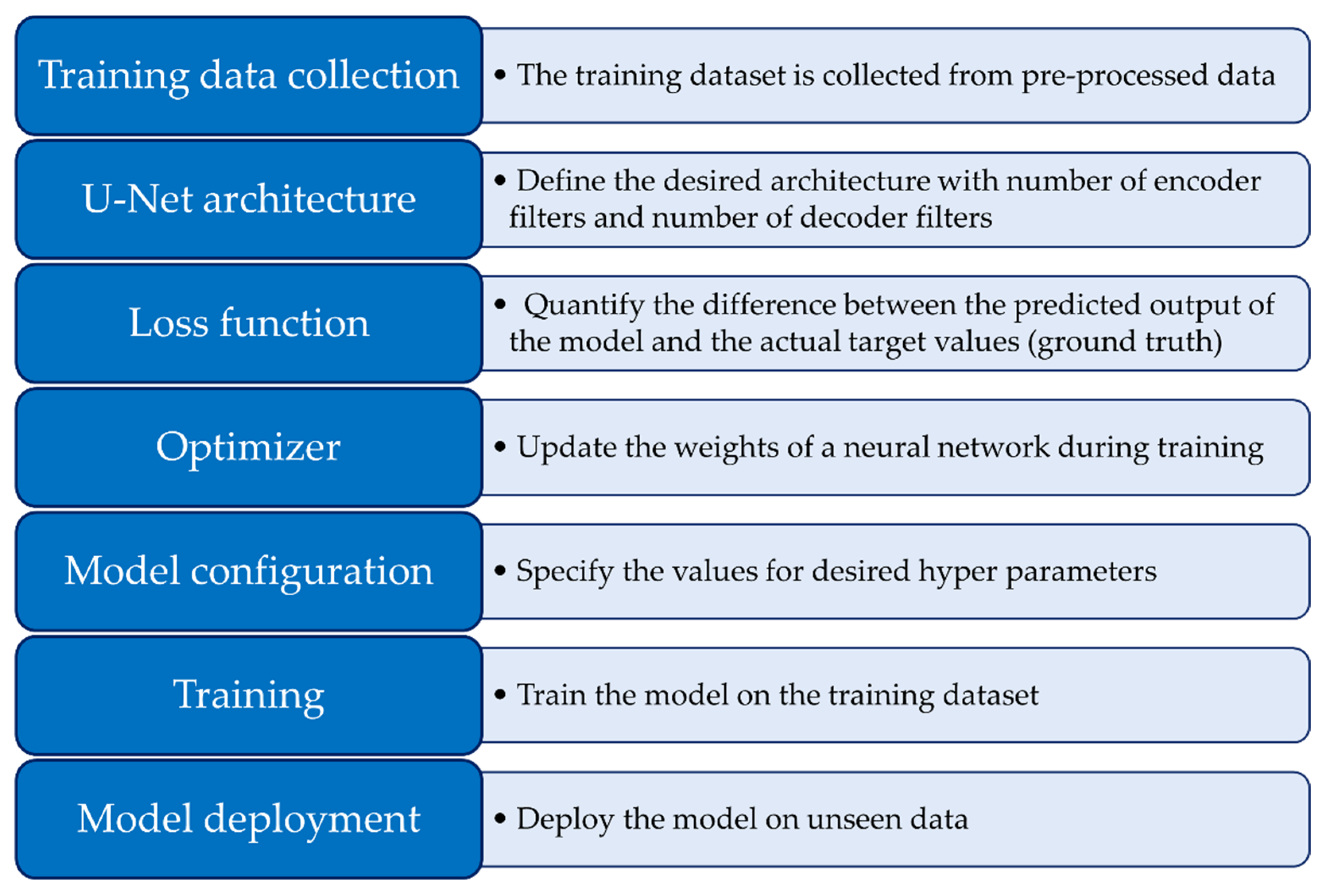
Figure 11.
Processing pipeline employed for U-Net segmentation, delineating the sequential steps and critical components integral to the methodology.
Figure 11.
Processing pipeline employed for U-Net segmentation, delineating the sequential steps and critical components integral to the methodology.
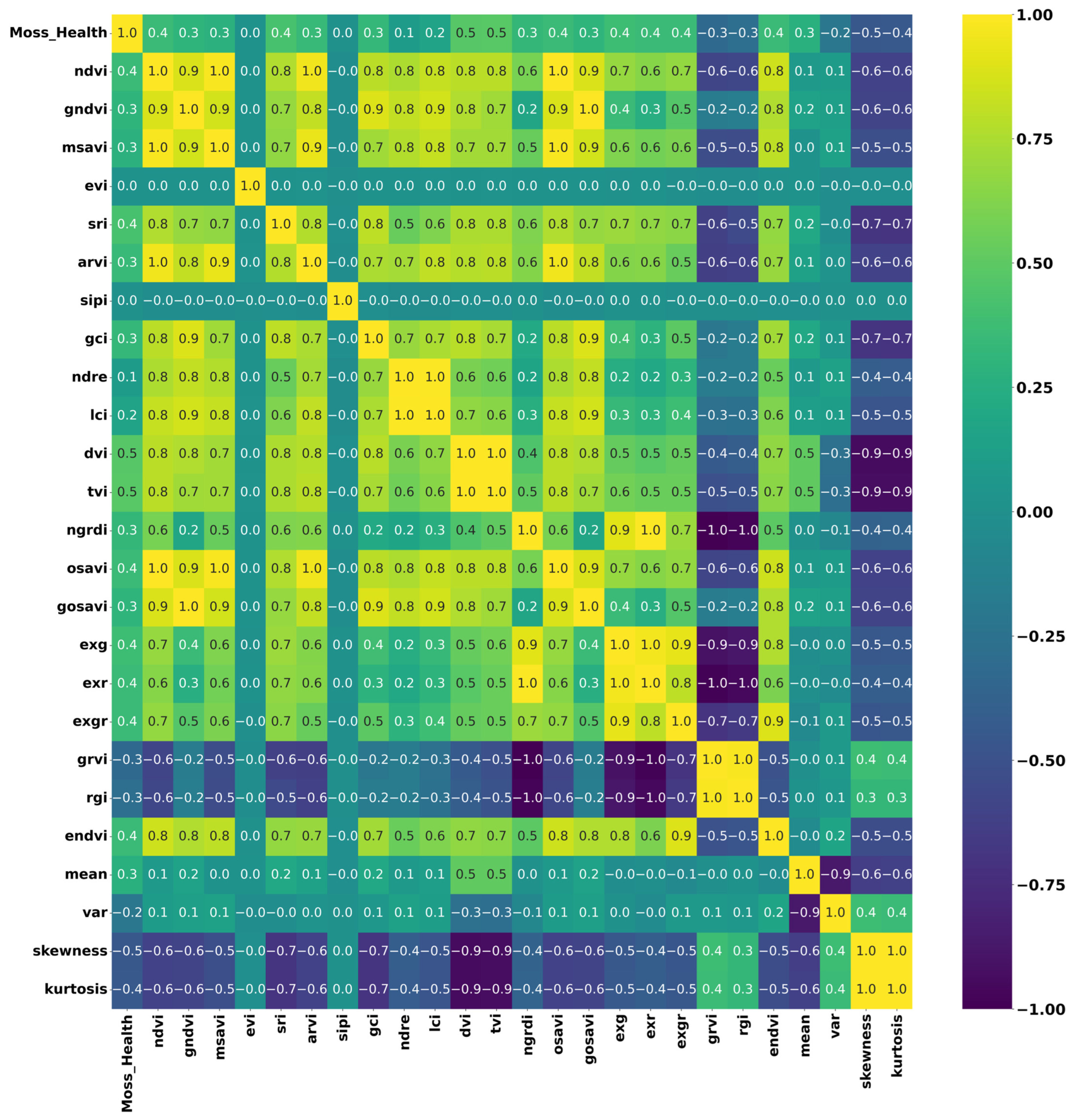
Figure 12.
Correlation matrix heatmap depicting the interrelationships among various vegetation indices used in the XGBoost model training for segmenting the healthy condition of moss and lichen. The colour intensity in the heatmap indicates the strength and direction of the correlations between different indices and statistical measures.
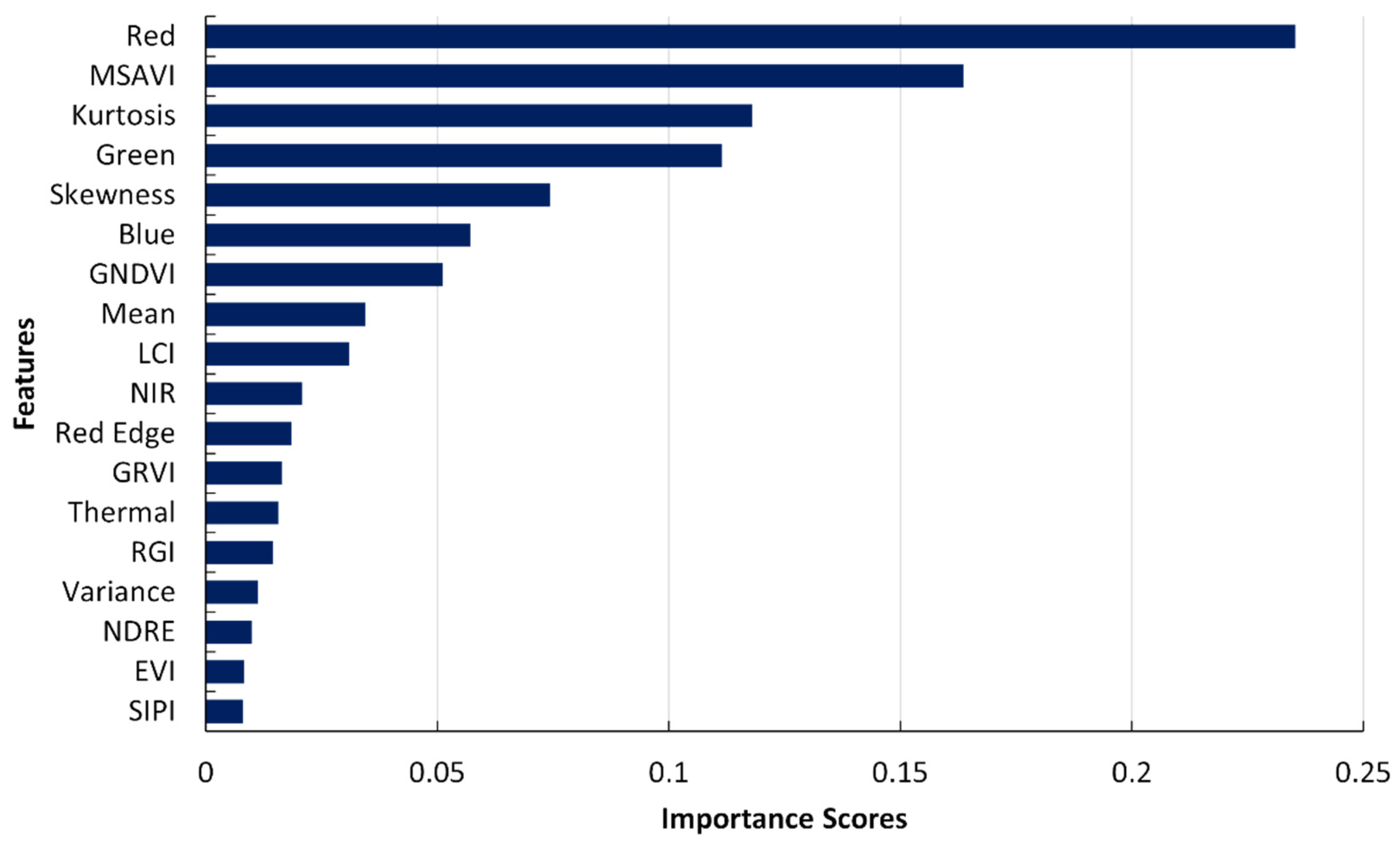
Figure 13.
Bar diagram of feature ranking, displaying the importance of different features in the XGBoost model’s prediction.
Figure 13.
Bar diagram of feature ranking, displaying the importance of different features in the XGBoost model’s prediction.
Figure 14.
Normalised confusion Matrix Heatmap representing the classification performance of XGBoost across five classes.
Figure 14.
Normalised confusion Matrix Heatmap representing the classification performance of XGBoost across five classes.
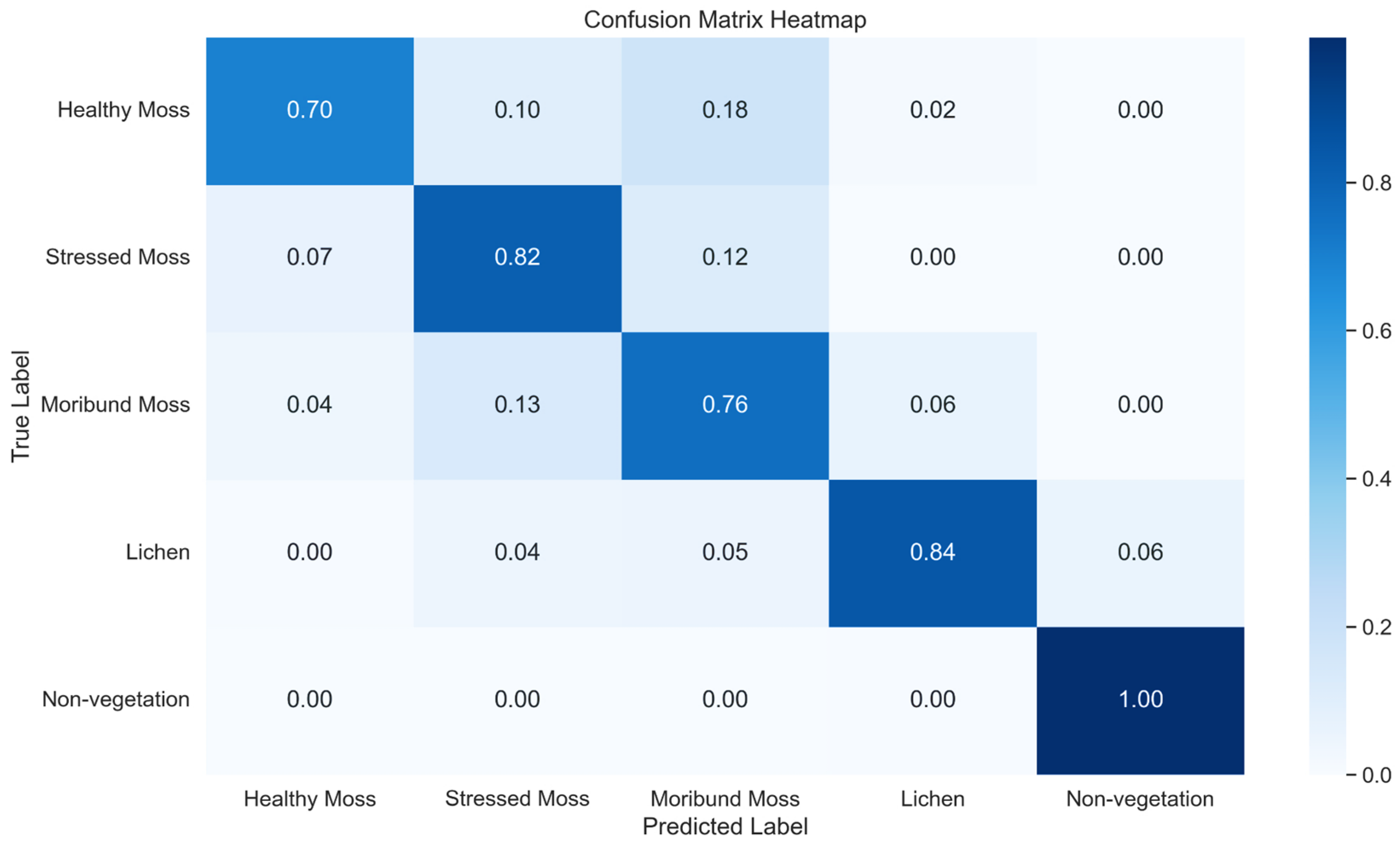
Figure 15.
Normalised confusion Matrix Heatmap representing the classification performance of U-Net across five classes using method 1.
Figure 15.
Normalised confusion Matrix Heatmap representing the classification performance of U-Net across five classes using method 1.
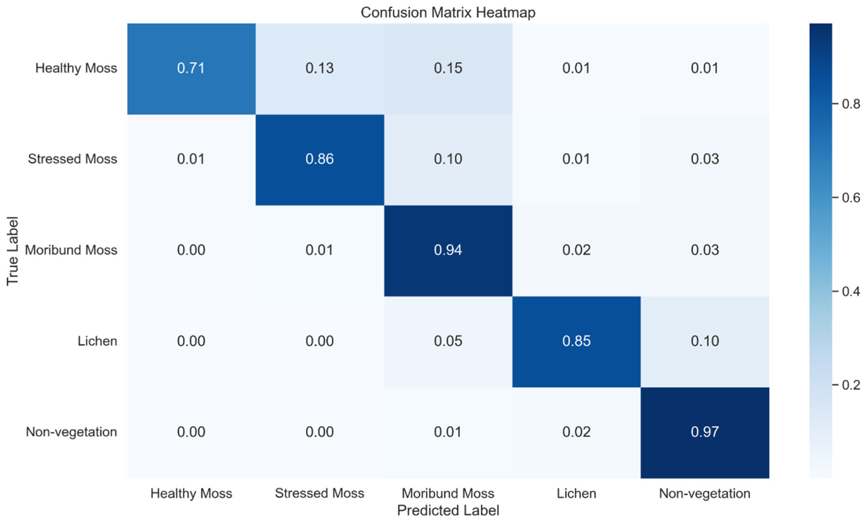
Figure 16.
Normalised confusion Matrix Heatmap representing the classification performance of a U-Net across five classes using method 2.
Figure 16.
Normalised confusion Matrix Heatmap representing the classification performance of a U-Net across five classes using method 2.
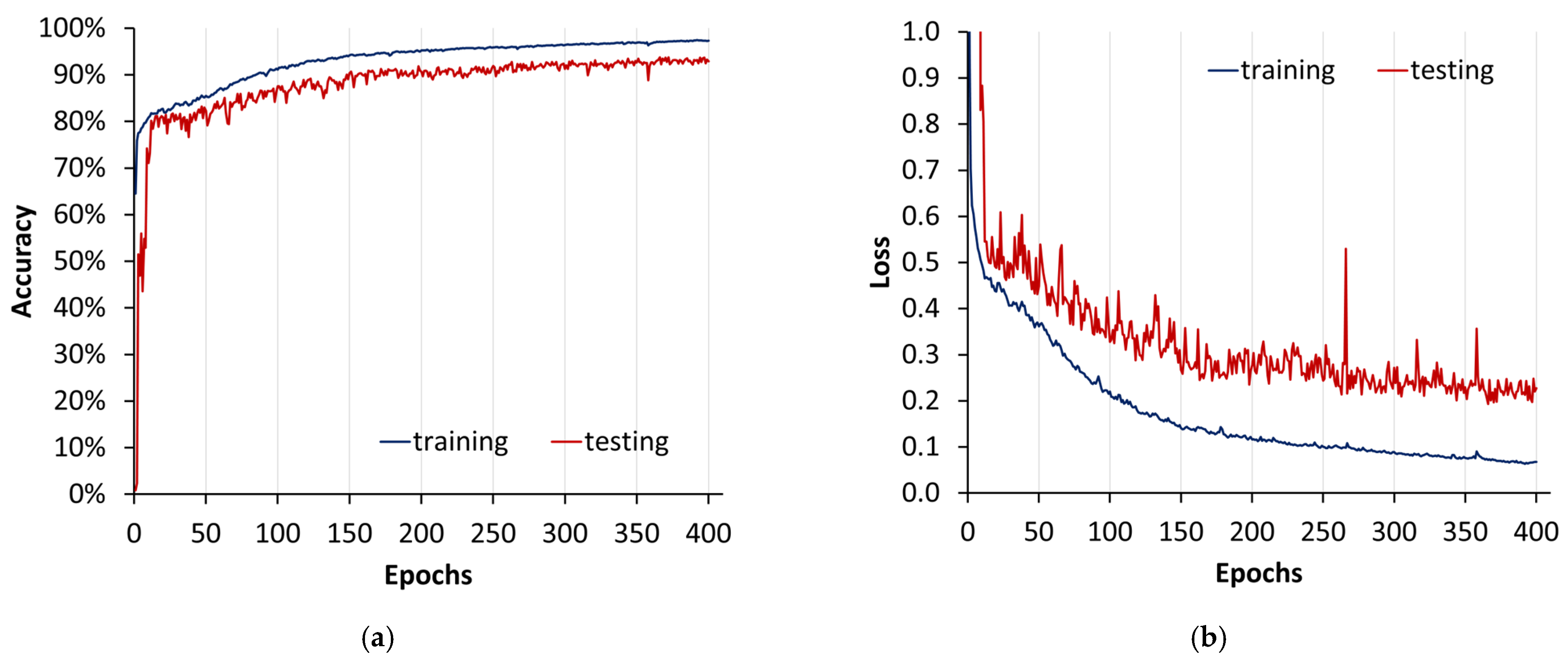
Figure 17.
U-Net model training plot from method 2: (a) accuracy; (b) loss. This visual representation spans epochs 0 to 400, providing an insight into the evolution of the model’s performance over a training period.
Figure 17.
U-Net model training plot from method 2: (a) accuracy; (b) loss. This visual representation spans epochs 0 to 400, providing an insight into the evolution of the model’s performance over a training period.
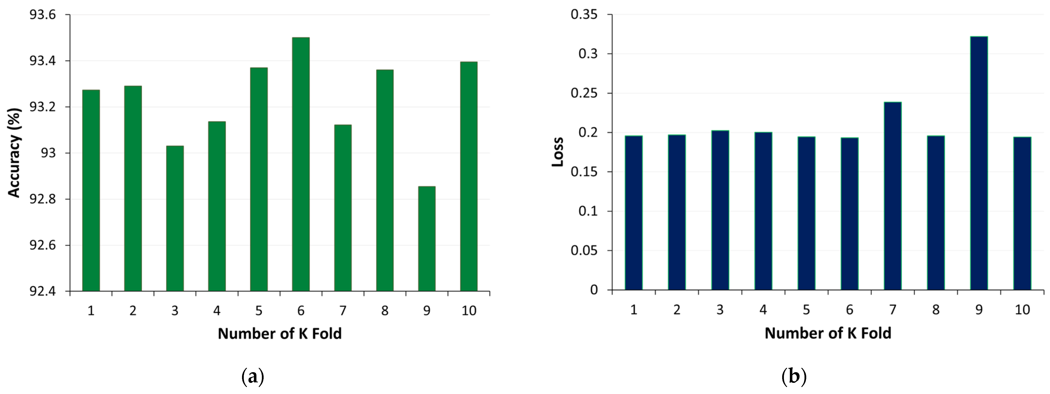
Figure 18.
K-fold cross validation for U-Net model using method 2: (a) accuracy, (b) loss.
Figure 18.
K-fold cross validation for U-Net model using method 2: (a) accuracy, (b) loss.
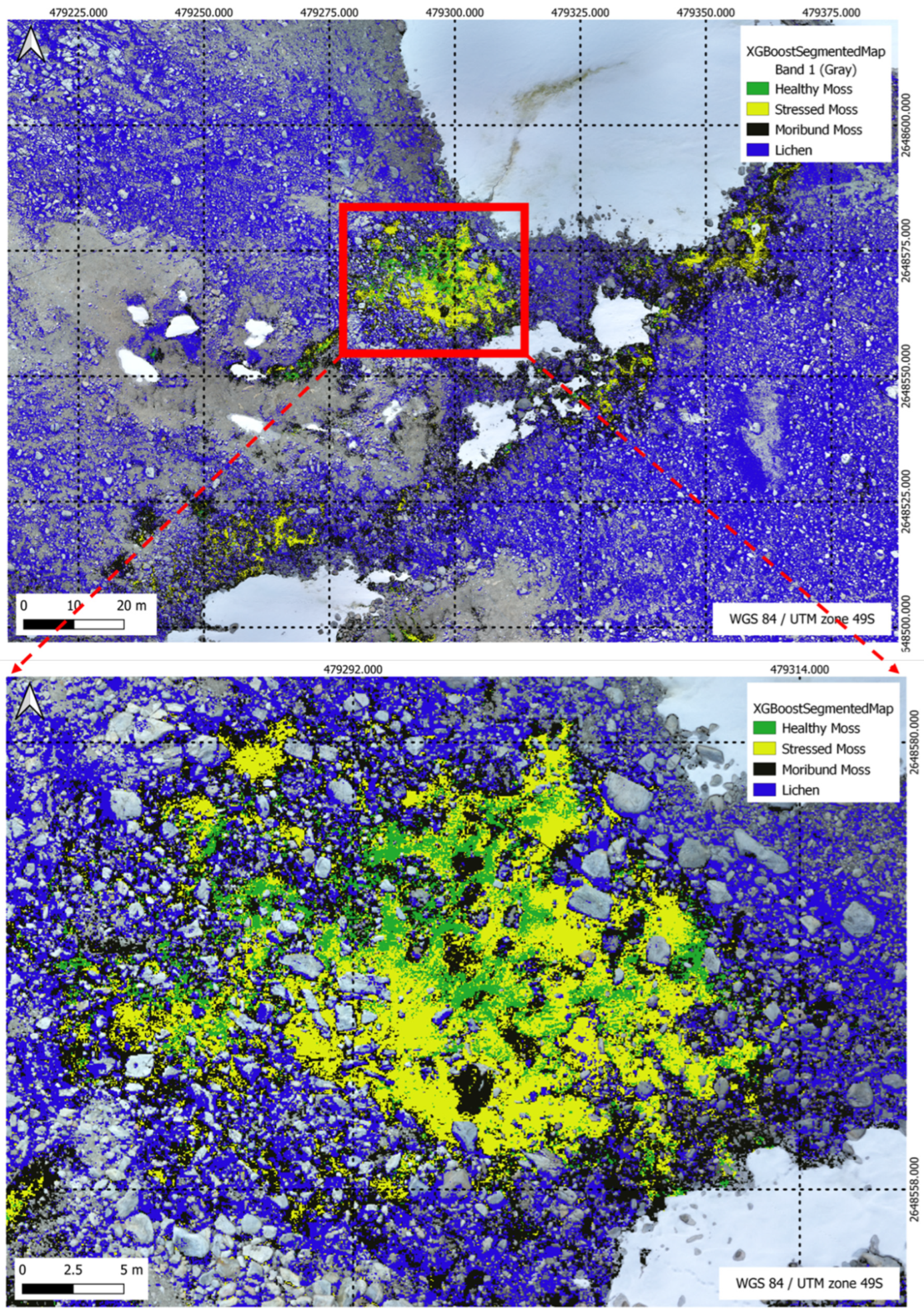
Figure 19.
XGBoost Segmentation results for a multi-class scenario, highlighting the model’s classification outcomes across five distinct classes in the segmentation task.
Figure 19.
XGBoost Segmentation results for a multi-class scenario, highlighting the model’s classification outcomes across five distinct classes in the segmentation task.
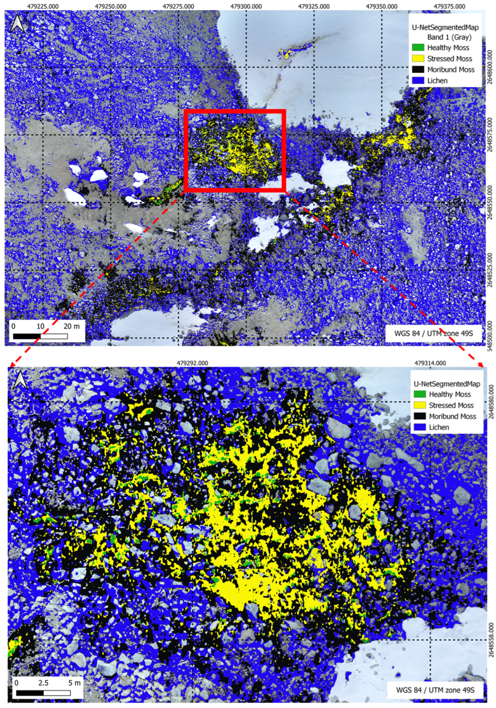
Figure 20.
U-Net Segmentation results (method 2) for a multi-class scenario, highlighting the model’s classification outcomes across five distinct classes in the segmentation task.
Figure 20.
U-Net Segmentation results (method 2) for a multi-class scenario, highlighting the model’s classification outcomes across five distinct classes in the segmentation task.
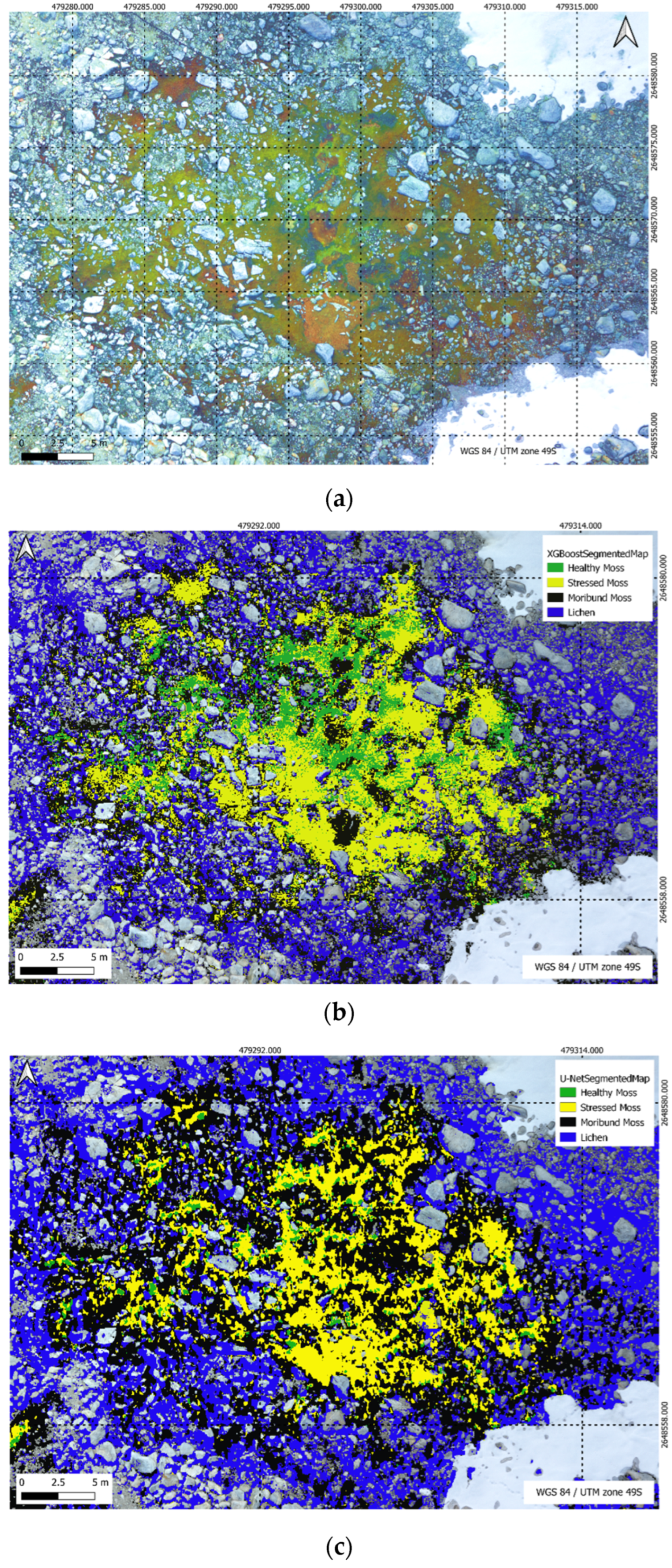
Figure 21.
(a) High resolution RGB image; (b) U-Net segmentation; (c) XGBoost segmentation.
Figure 21.
(a) High resolution RGB image; (b) U-Net segmentation; (c) XGBoost segmentation.
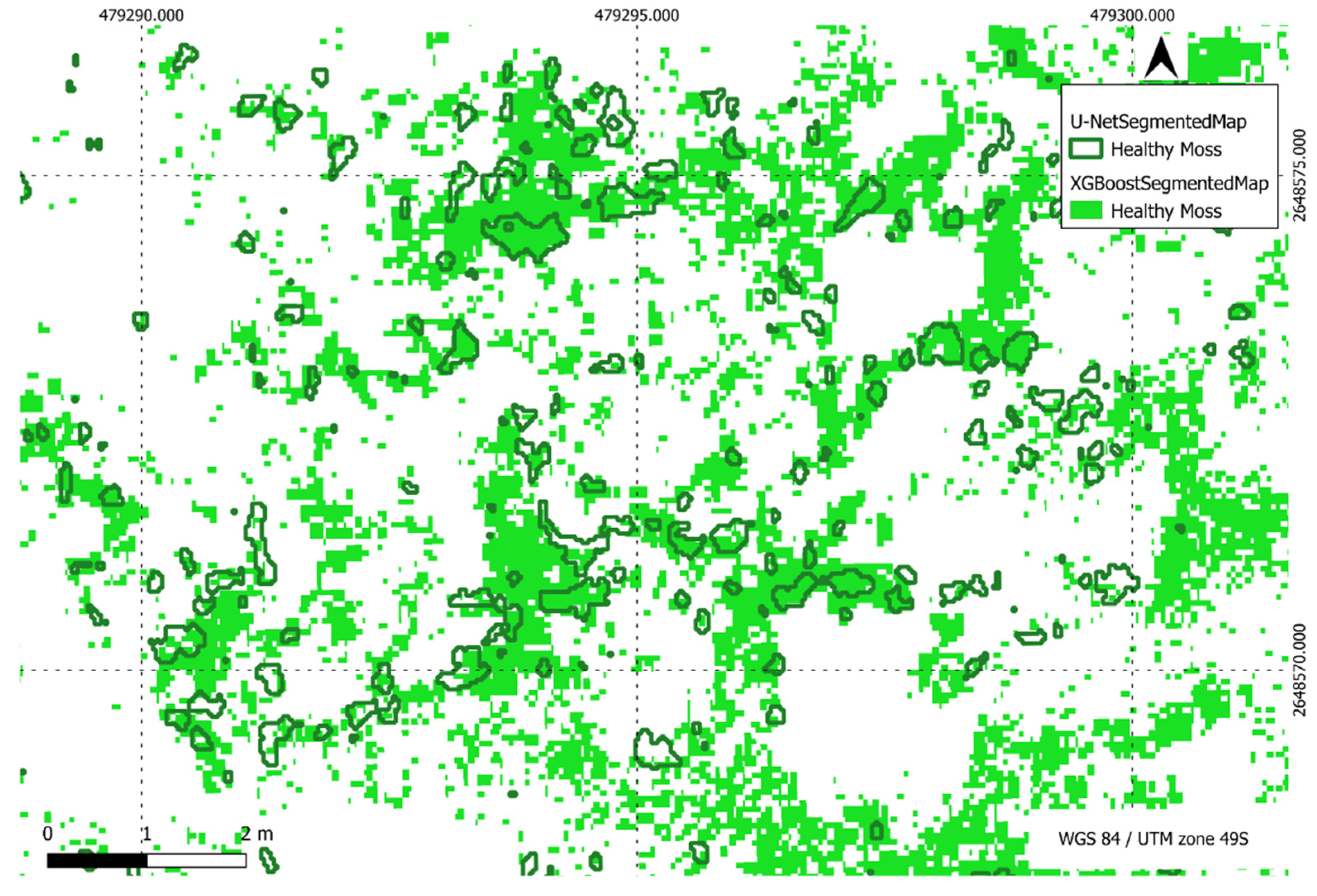
Figure 22.
Comparison of XGBoost and U-Net predictions of healthy moss in a region of interest.
Figure 22.
Comparison of XGBoost and U-Net predictions of healthy moss in a region of interest.
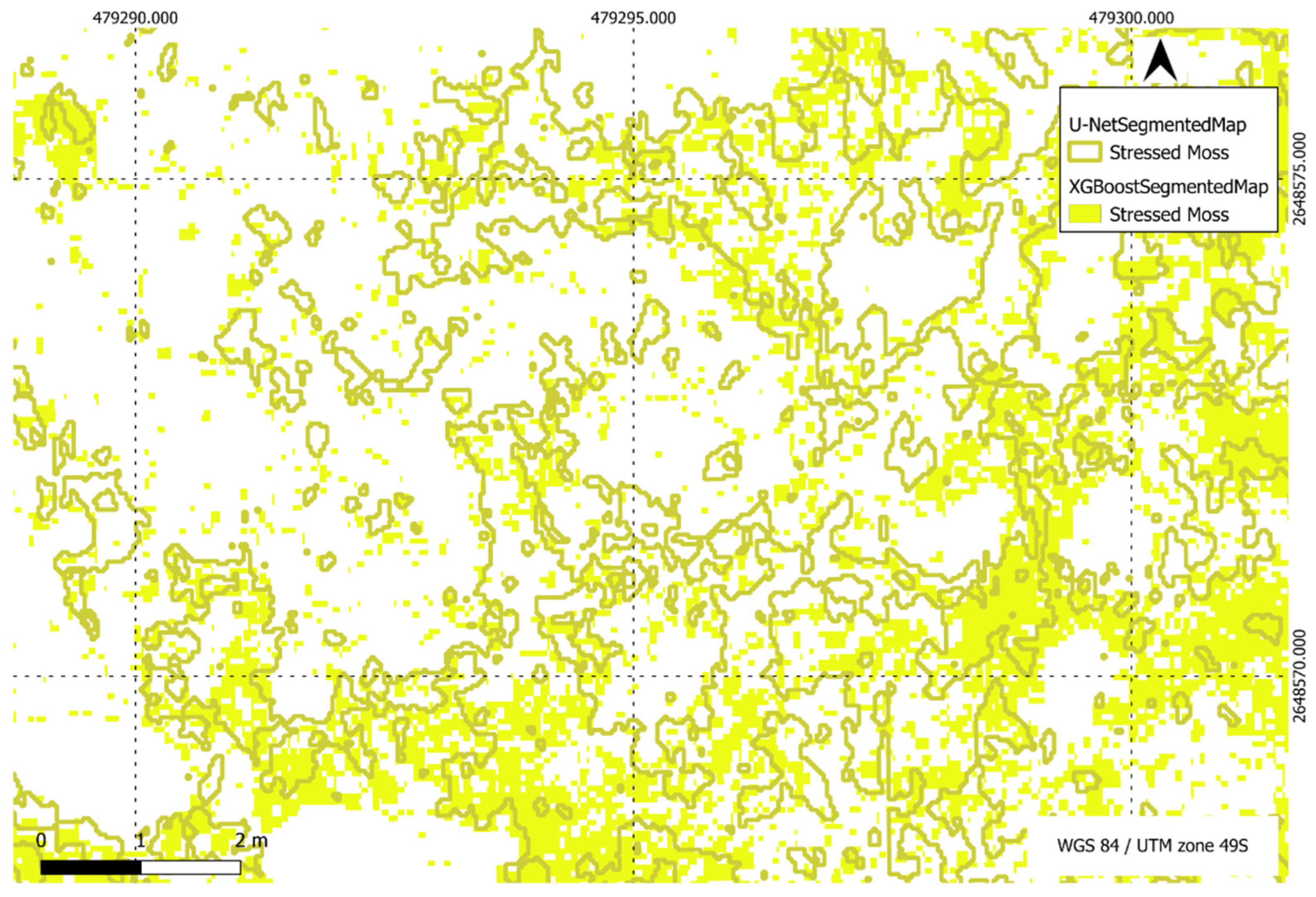
Figure 23.
Comparison of XGBoost and U-Net predictions of stressed moss in a region of interest.
Figure 23.
Comparison of XGBoost and U-Net predictions of stressed moss in a region of interest.
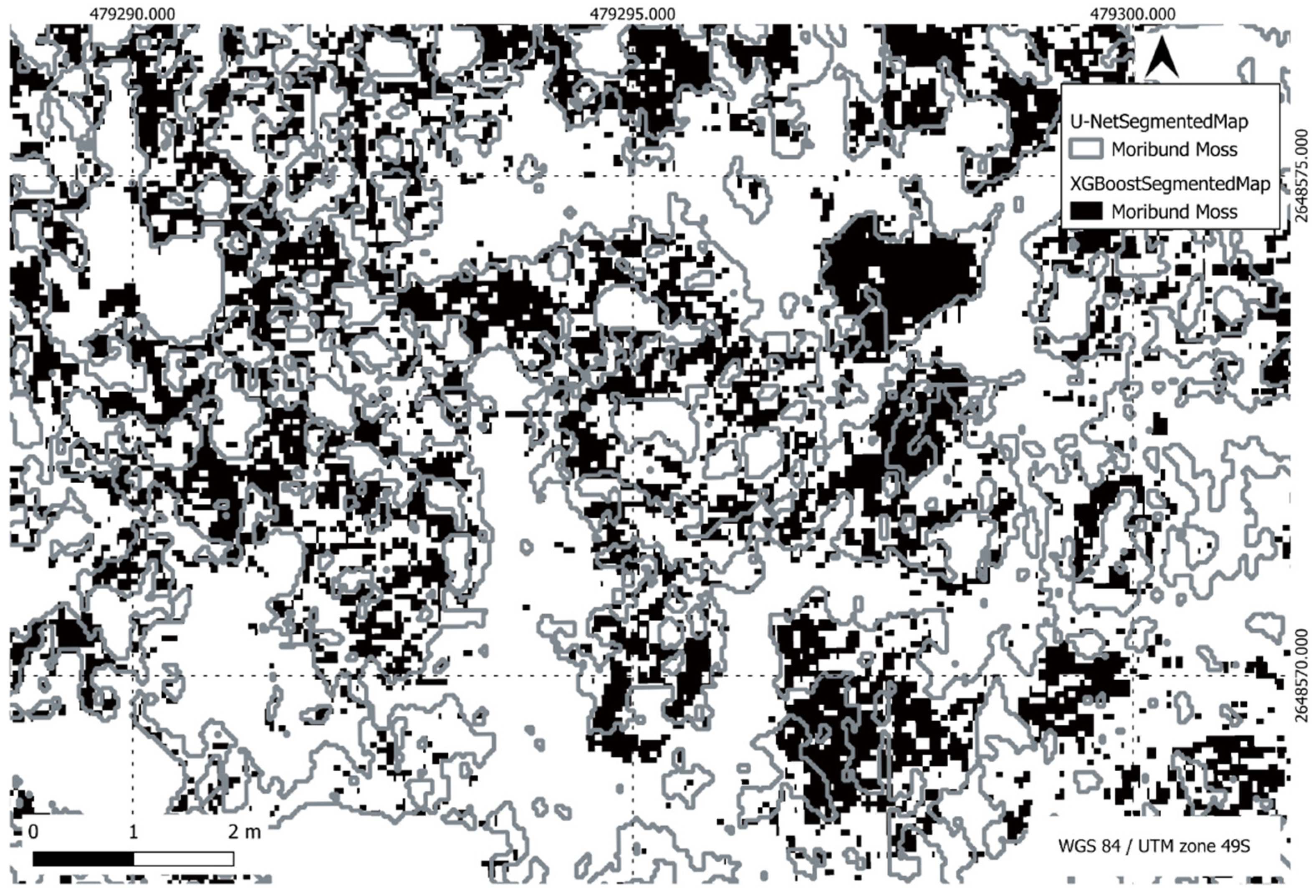
Figure 24.
Comparison of XGBoost and U-Net predictions of moribund moss in a region of interest.
Figure 24.
Comparison of XGBoost and U-Net predictions of moribund moss in a region of interest.
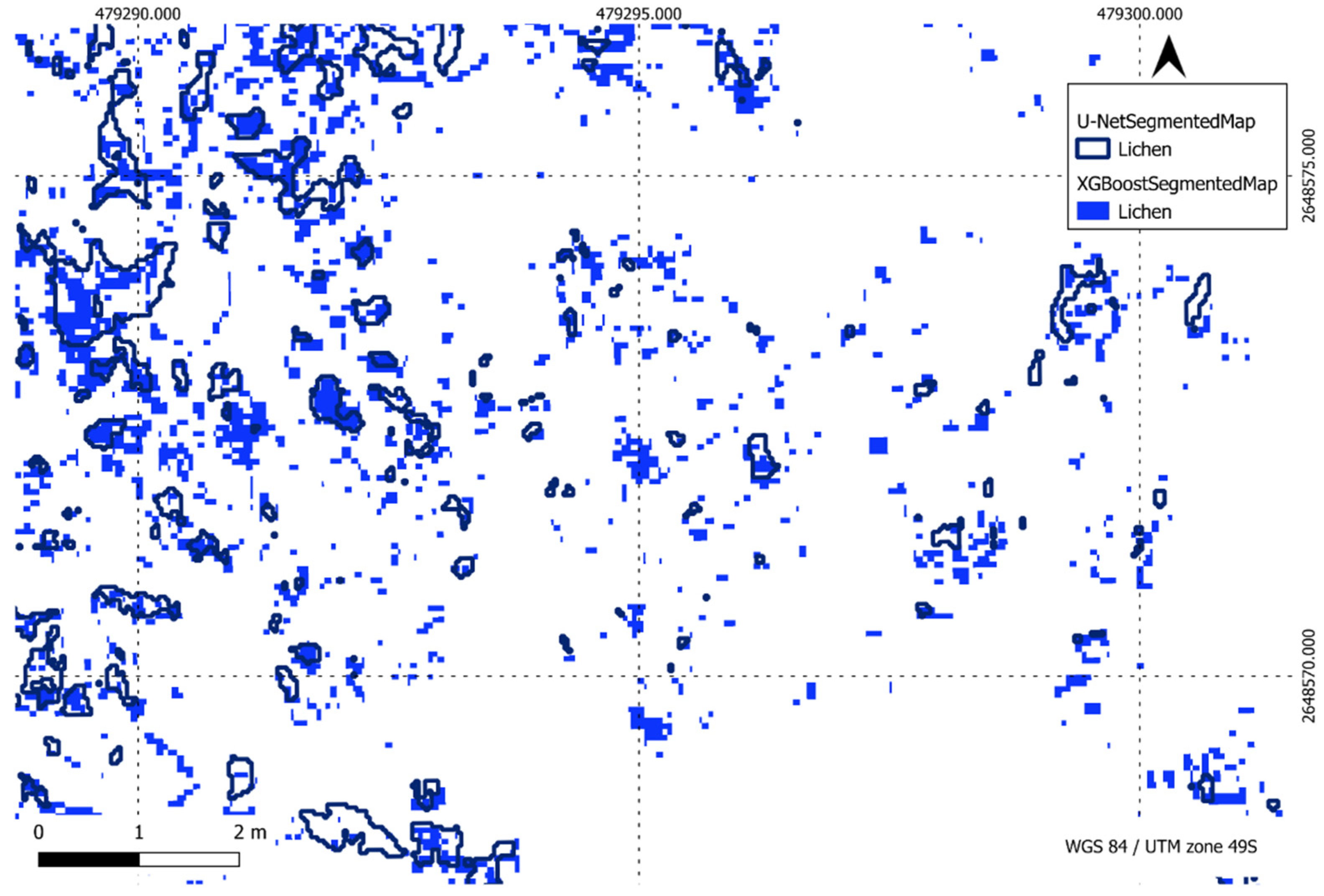
Figure 25.
Comparison of XGBoost and U-Net predictions of lichen in a region of interest.
Figure 25.
Comparison of XGBoost and U-Net predictions of lichen in a region of interest.
Table 1.
Key specifications of different aircraft used in this study.
Table 1.
Key specifications of different aircraft used in this study.
| Specifications | BMR3.9RTK | DJI Mini 3 Pro |
|---|
| Weight | 12 kg,
Maximum take-off weight of 14 kg | Less than 249 g |
| Battery type | Two six cell LiPo batteries | Li-ion |
| Flight time | 30 min with dual payload capability | 34 min (with Intelligent Flight Battery measured while flying at 21.6 kph in windless conditions) |
Table 2.
Key specifications of different sensors used in this study.
Table 2.
Key specifications of different sensors used in this study.
| Specifications | MicaSense Altum | Sony Alpha 5100 | DJI Mini 3 Pro Inbuilt Camera |
|---|
| Number of bands | Five multispectral and a thermal band | Three | Three |
| Bands | blue, green, red, red-edge, and near-infrared, short wave infrared (thermal) | blue, green, red | blue, green, red |
| Resolution | Multispectral: 3.2 megapixels (MPs) and Thermal: 320 × 256 pixels. | 24.3 MPs | 48 MPs |
| Field of view | 50.2° × 38.4° | 83° | 82.1° |
Table 3.
Comprehensive overview of moss health states and descriptions.
Table 3.
Comprehensive overview of moss health states and descriptions.
| Health Status of Moss | Description |
|---|
| Healthy | Moss in good health exhibits shades ranging from dark (ms_gr) to bright green (ms_bg), indicating healthy chloroplasts and plenty of chlorophyll. It is typically found in regions with consistent meltwater availability. |
| Stressed | Moss undergoing stress experiences a reduction in chlorophyll pigments, appearing red or brown (ms_rd) due to the presence of carotenoids and other photoprotective pigments, as noted by Waterman et al. (2018). Stressors such as drought or intense solar radiation can contribute to this condition. However, if the stress is reversed, the moss turf has the potential to regain its green colour, facilitated by the formation of new leaves [4]. |
| Moribund | Intense or prolonged stress leads to the moribund state of moss, where leaves undergo pigment loss, rendering them grey in colour (ms_bw and ms_mm). Additionally, these stressed moss specimens may become encrusted with lichens. |
Table 4.
Comprehensive overview of the various spectral indices utilised in the current study, offering a detailed compilation of the specific indices employed to analyse and interpret spectral data.
Table 4.
Comprehensive overview of the various spectral indices utilised in the current study, offering a detailed compilation of the specific indices employed to analyse and interpret spectral data.
| Spectral Indices | Formula | Literature Review |
|---|
| Normalised Difference Vegetation Index (NDVI) | | [43] |
| Green Normalised Difference Vegetation Index (GNDVI) | | [44,45,46] |
| Modified Soil-Adjusted Vegetation Index (MSAVI) | | [47] |
| Enhanced Vegetation Index (EVI) | | [48] |
| Simple Ratio Index (SRI) | | [49] |
| Atmospherically Resistant Vegetation Index (ARVI) | | [47] |
| Structure Insensitive Pigment Index (SIPI) | | [50] |
| Green Chlorophyll Index (GCI) | | [51,52] |
| Normalised Difference Red Edge Index (NDRE) | | [53,54,55] |
| Leaf Chlorophyll Index (LCI) | | [48] |
| Difference Vegetation Index (DVI) | | [46,51,56] |
| Triangular Vegetation Index (TVI) | | [48] |
| Normalised Green Red Difference (NGRDI) | | [46,57] |
| Optimised Soil-Adjusted Vegetation Index (OSAVI) | | [58] |
| Green Optimised Soil Adjusted Vegetation Index (GOSAVI) | | [58] |
| Excess Green (EXG) | | [59] |
| Excess Red (EXR) | | [59] |
| Excess Green Red (EXGR) | | [59] |
| Red Green Index (RGI) | | [59] |
| Green Red Vegetation Index (GRVI) | | [59] |
| Enhanced Normalised Difference Vegetation Index (ENDVI) | | [50] |
Table 5.
Parameter tuning for U-Net training.
Table 5.
Parameter tuning for U-Net training.
| Preprocessing | Patch size | 32, 64, 128, 256 |
| Overlap | 0.1, 0.2, 0.3 |
| Low pass filter | Without filter, 3 × 3, 5 × 5, 7 × 7 |
| Gaussian blur filter | Without filter, 3 × 3, 5 × 5, 7 × 7 |
| Train test split | 20%, 25%, 30% |
| Model Architecture | Convolution layers | 8–1024, 16–1024, 32–1024, 64–1024, 128–1024, 16–512, 32–512, 128–512, 8–256, 16–256, 32–256 |
| Kernal size | 1 × 1, 3 × 3, 5 × 5 |
| Dropout | 0.1, 0.2 |
| Model compile and Training | Learning rate | 0.1, 0.01, 0.001, 0.0001 |
| Batch size | 10, 15, 20, 25, 30, 35 |
| Epochs | 50, 75, 100, 150, 200, 250, 300, 400 |
Table 6.
Classification Report summarising key metrics for an XGBoost model, including precision, recall, and F1-score, across five classes.
Table 6.
Classification Report summarising key metrics for an XGBoost model, including precision, recall, and F1-score, across five classes.
| Classes | Precision | Recall | F1-Score |
|---|
| Healthy Moss | 0.86 | 0.71 | 0.78 |
| Stressed Moss | 0.86 | 0.83 | 0.85 |
| Moribund Moss | 0.88 | 0.92 | 0.90 |
| Lichen | 0.94 | 0.91 | 0.93 |
| Non-Vegetation | 1.00 | 1.00 | 1.00 |
Table 7.
Classification Report summarising key metrics for a U-Net model, including precision, recall, and F1-score, across five classes using method 1.
Table 7.
Classification Report summarising key metrics for a U-Net model, including precision, recall, and F1-score, across five classes using method 1.
| Classes | Precision | Recall | F1-Score | IoU |
|---|
| Healthy Moss | 0.74 | 0.70 | 0.72 | 0.56 |
| Stressed Moss | 0.69 | 0.82 | 0.75 | 0.60 |
| Moribund Moss | 0.77 | 0.76 | 0.77 | 0.63 |
| Lichen | 0.86 | 0.84 | 0.85 | 0.74 |
| Non-Vegetation | 1.00 | 1.00 | 1.00 | 0.99 |
Table 8.
Classification Report summarising key metrics for a U-Net model, including precision, recall, and F1-score, across five classes using method 2.
Table 8.
Classification Report summarising key metrics for a U-Net model, including precision, recall, and F1-score, across five classes using method 2.
| Classes | Precision | Recall | F1-Score | IoU |
|---|
| Healthy Moss | 0.94 | 0.71 | 0.81 | 0.67 |
| Stressed Moss | 0.86 | 0.86 | 0.86 | 0.75 |
| Moribund Moss | 0.87 | 0.94 | 0.90 | 0.82 |
| Lichen | 0.95 | 0.85 | 0.90 | 0.82 |
| Non-Vegetation | 0.94 | 0.97 | 0.96 | 0.92 |
Table 9.
Class distribution in the target area (931.12 m2) using XGBoost and U-Net Models.
Table 9.
Class distribution in the target area (931.12 m2) using XGBoost and U-Net Models.
| Class | XGBoost | U-Net |
|---|
| Healthy Moss | 6% | 3% |
| Stressed Moss | 15% | 12% |
| Moribund Moss | 20% | 30% |
| Lichen | 21% | 21% |


 ,
, 


