Funding
The author reports that no funding was received for this study. Data used in the preparation of this article were obtained on 15 July 2024 from the Parkinson’s Progression Markers Initiative (PPMI). PPMI—a public-private partnership—is funded by the Michael J. Fox Foundation for Parkinson’s Research and funding partners, including 4D Pharma, Abbvie, AcureX, Allergan, Amathus Therapeutics, Aligning Science Across Parkinson’s, AskBio, Avid Radiopharmaceuticals, BIAL, Biogen, Biohaven, BioLegend, BlueRock Therapeutics, Bristol-Myers Squibb, Calico Labs, Celgene, Cerevel Therapeutics, Coave Therapeutics, DaCapo Brainscience, Denali, Edmond J. Safra Foundation, Eli Lilly, Gain Therapeutics, GE HealthCare, Genentech, GSK, Golub Capital, Handl Therapeutics, Insitro, Janssen Neuroscience, Lundbeck, Merck, Meso Scale Discovery, Mission Therapeutics, Neurocrine Biosciences, Pfizer, Piramal, Prevail Therapeutics, Roche, Sanofi, Servier, Sun Pharma Advanced Research Company, Takeda, Teva, UCB, Vanqua Bio, Verily, Voyager Therapeutics, the Weston Family Foundation, and Yumanity Therapeutics.
Figure 1.
Schematic representation of basal ganglia circuitry and its disruption in Parkinson’s disease (PD). The diagram highlights the structures involved in movement regulation: the substantia nigra (SN), striatum (D1 and D2 pathways), globus pallidus externus (GPe) and internus (GPi), subthalamic nucleus (STN), thalamus, and frontal motor cortex (M1 and SMC). Green arrows indicate excitatory pathways, while red arrows represent inhibitory pathways. In PD, the loss of dopamine-producing neurons in the substantia nigra (SNc) disrupts the balance between the “GO” (direct) and “noGO” (indirect) pathways, leading to overactivation of the GPi and increased inhibition of the thalamus, eventually impairing movement signals to the motor cortex. Based on work by Przybyszewski et al. (2021) [
20].
Figure 2.
This 3D reconstruction illustrates the segmentation of selected brain regions of interest (ROIs) based on FreeSurfer processing. The segmented structures include the thalamus, hippocampus, amygdala, caudate, putamen, pallidum, cerebellum, and cerebrospinal fluid (CSF). Each structure is represented by a distinct color. In the center of each segmented structure, a central point (centroid) is displayed, representing the geometric center of that region.
Figure 3.
The Euclidean distance (considered as Minkowski distance with the parameter p = 2) represents the straight-line distance between the centroids of each structure (A) relative to the thalamus (B) in a three-dimensional space, providing a measure of physical separation. The Cosine distance is the angular difference between the vectors originating from the thalamus to the structures, showing their relative orientation in space.
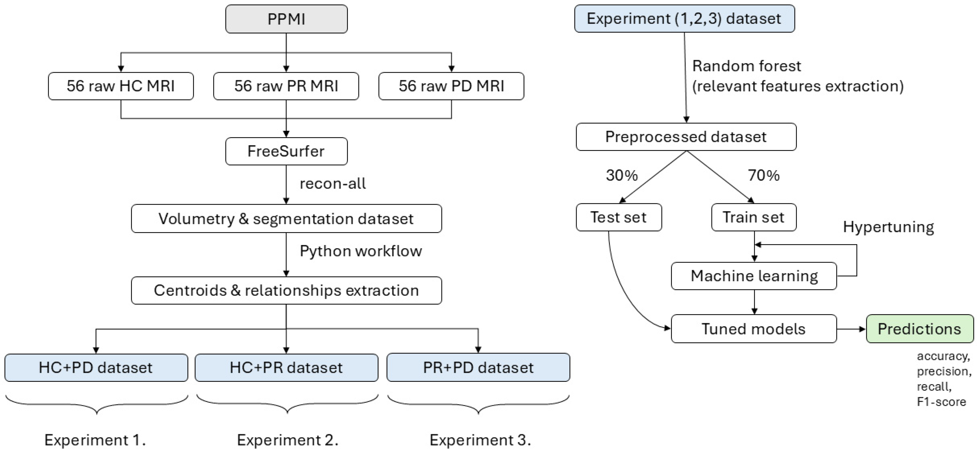
Figure 4.
The workflow illustrates the processing pipeline starting from raw MRI data obtained from the PPMI dataset, including 56 healthy controls (HCs), 56 prodromal (PR), and 56 Parkinson’s disease (PD) subjects. The data are processed using FreeSurfer to extract volumetric and centroid-based features, which are then organized into three experimental datasets. In each experiment, Random Forest is applied for feature selection. This is followed by a 30/70 train–test split, hypertuning, and machine learning model training to generate predictions for each experiment.
Figure 5.
Thalamus volume distribution. The boxplot (left) shows the distribution of thalamus volumes for the control, Parkinson’s disease, and prodromal groups. The density plot (right) shows the kernel density estimates for the thalamus volumes in each group. The circles in the boxplot represent outliers beyond 1.5 times the IQR.
Figure 6.
Left Hippocampus—Euclidean distance. The boxplot (left) shows the distribution of the normalized Euclidean distances between the left hippocampus and thalamus across the control, Parkinson’s disease, and prodromal groups. The density plot (right) illustrates the kernel density estimates of the distances for each group, showing variability in the distance between the left hippocampus and thalamus. The circles in the boxplot represent outliers beyond 1.5 times the IQR.
Figure 7.
Left Hippocampus—Cosine distance. The boxplot (left) illustrates the distribution of Cosine distances between the left hippocampus and thalamus across the control, Parkinson’s disease, and prodromal groups. The density plot (right) shows the kernel density estimates of the Cosine distances for each group, showing variability in angular positioning of the left hippocampus with respect to the thalamus. The circles in the boxplot represent outliers beyond 1.5 times the IQR.
Figure 8.
ROC curves and confusion matrices for classification of HC and PD. The top row shows the receiver operating characteristic (ROC) curves for the Random Forest (left), Support Vector Classifier (middle), and Logistic Regression (right) models. The area under the curve (AUC) values are presented for each model, with Logistic Regression achieving the highest AUC (0.89). The bottom row presents the corresponding confusion matrices for each model, illustrating the distribution of correctly and incorrectly classified participants for healthy controls and Parkinson’s patients. Logistic Regression achieved the best performance with 15 true positives and only 2 false negatives.
Figure 9.
ROC curves and confusion matrices for classification of HC and PR. The top row shows the receiver operating characteristic (ROC) curves for the Random Forest (left), Support Vector Classifier (middle), and Logistic Regression (right) models. The area under the curve (AUC) values are presented for each model, with SVC achieving the highest AUC (0.99). The bottom row presents the corresponding confusion matrices for each model, illustrating the distribution of correctly and incorrectly classified participants for healthy controls and prodromal cases. The numbers in the figure represent the counts of correctly and incorrectly classified samples for each group. The Logistic Regression and SVC models showed the best performance, with both correctly classifying all prodromal cases and having only four and five false positives, respectively.
Figure 10.
ROC curves and confusion matrices for classification of PD and PR. The top row shows the receiver operating characteristic (ROC) curves for the Random Forest (left), Support Vector Classifier (middle), and Logistic Regression (right) models. The area under the curve (AUC) values are presented for each model, with Logistic Regression achieving the highest AUC (0.73). The bottom row presents the corresponding confusion matrices for each model, illustrating the distribution of correctly and incorrectly classified participants for Parkinson’s disease and prodromal cases. The numbers in the figure represent the counts of correctly and incorrectly classified samples for each group. Logistic Regression showed the best performance, correctly classifying 15 prodromal cases and 9 Parkinson’s cases, while Random Forest and SVC demonstrated lower overall accuracy with more misclassifications.
Table 1.
Parameters of selected MRI scans and sensors obtained from the PPMI study.
Table 1.
Parameters of selected MRI scans and sensors obtained from the PPMI study.
| Parameter | Value |
|---|
| Sensor | MRI |
| Group | Control, Prodromal, Parkinson |
| Visit | Baseline (BL) |
| Acquisition Plane | Sagittal |
| Field Strength | 3.0 Tesla |
| Slice Thickness | 1.0 mm |
| Sequencing | 3D T1-weighted or MPRAGE GRAPPA |
| Weighting | T1 |
Table 2.
MRI Scanners and sequences used in the study.
Table 2.
MRI Scanners and sequences used in the study.
| Manufacturer | Model | Sequence | HC (n = 56) | PD (n = 56) | PR (n = 56) |
|---|
| Siemens | TrioTim | MPRAGE GRAPPA | 46 | 0 | 0 |
| Siemens | Verio | MPRAGE GRAPPA | 9 | 0 | 0 |
| GE | SIGNA Architect | SAG 3D T1-weighted | 1 | 0 | 0 |
| GE | DISCOVERY MR750 | 3D T1-weighted | 0 | 5 | 10 |
| GE | SIGNA Architect | 3D T1-weighted | 0 | 12 | 17 |
| Philips | Achieva | 3D T1-weighted | 0 | 3 | 3 |
| Philips | Achieva dStream | 3D T1-weighted | 0 | 34 | 26 |
| Toshiba | Vantage Elan | 3D T1-weighted | 0 | 2 | 0 |
Table 3.
The table presents the mean ± standard deviation for demographic and clinical parameters, including sex, age, and UPDRS3 scores, across the healthy control (CONTROL), Parkinson’s disease (PARKINSON), and prodromal (PRODROMAL) groups.
Table 3.
The table presents the mean ± standard deviation for demographic and clinical parameters, including sex, age, and UPDRS3 scores, across the healthy control (CONTROL), Parkinson’s disease (PARKINSON), and prodromal (PRODROMAL) groups.
| Parameter | p-Value | CONTROL (n = 56) | PARKINSON (n = 56) | PRODROMAL (n = 56) |
|---|
| Age, years | 0.065 | 61.536 ± 11.492 | 61.839 ± 10.986 | 66.339 ± 6.162 |
| Sex, female | 0.260 | 0.321 ± 0.471 | 0.429 ± 0.499 | 0.250 ± 0.437 |
| UPDRS | 0.000 | 0.786 ± 1.670 | 23.893 ± 11.474 | 4.857 ± 5.910 |
Table 4.
The table presents statistical comparisons (FDR-adjusted) between the volumes of selected brain structures across the healthy control (HC), Parkinson’s disease (PD), and prodromal (PR) groups. Bold values indicate statistically significant results.
Table 4.
The table presents statistical comparisons (FDR-adjusted) between the volumes of selected brain structures across the healthy control (HC), Parkinson’s disease (PD), and prodromal (PR) groups. Bold values indicate statistically significant results.
| Volume | ANOVA p-Value | HC vs. PD p-Value | HC vs. PR p-Value | PD vs. PR p-Value |
|---|
| Thalamus | 0.108 | 0.062 | 0.793 | 0.167 |
| Left-Hippocampus | 0.065 | 0.035 | 0.363 | 0.227 |
| Right-Hippocampus | 0.589 | 0.338 | 0.710 | 0.674 |
| Left-Amygdala | 0.001 | 0.002 | 0.002 | 0.799 |
| Right-Amygdala | 0.945 | 0.839 | 0.721 | 0.945 |
| Left-Caudate | 0.034 | 0.015 | 0.096 | 0.465 |
| Right-Caudate | 0.200 | 0.089 | 0.184 | 0.873 |
| Left-Putamen | 0.002 | 0.002 | 0.001 | 0.984 |
| Right-Putamen | 0.016 | 0.035 | 0.006 | 0.707 |
| Left-Pallidum | 0.167 | 0.124 | 0.089 | 0.945 |
| Right-Pallidum | 0.945 | 0.799 | 0.859 | 0.945 |
| Left-Accumbens | 0.001 | 0.001 | 0.001 | 0.859 |
| Right-Accumbens | 0.347 | 0.257 | 0.184 | 0.963 |
| Left-VentralDC | 0.003 | 0.002 | 0.051 | 0.227 |
| Right-VentralDC | 0.133 | 0.065 | 0.168 | 0.710 |
| 4th-Ventricle | 0.945 | 0.799 | 0.945 | 0.823 |
| Left-Cerebellum | 0.258 | 0.599 | 0.411 | 0.112 |
| Right-Cerebellum | 0.220 | 0.638 | 0.343 | 0.096 |
| CSF | 0.177 | 0.599 | 0.065 | 0.334 |
Table 5.
The table presents statistical comparisons (FDR-adjusted) between the Euclidean distances of selected brain structures and the thalamus across the healthy control (HC), Parkinson’s disease (PD), and prodromal (PR) groups. Bold values indicate statistically significant results.
Table 5.
The table presents statistical comparisons (FDR-adjusted) between the Euclidean distances of selected brain structures and the thalamus across the healthy control (HC), Parkinson’s disease (PD), and prodromal (PR) groups. Bold values indicate statistically significant results.
| Euclidean Distance. | ANOVA p-Value | HC vs. PD p-Value | HC vs. PR p-Value | PD vs. PR p-Value |
|---|
| Left-Hippocampus | 0.015 | 0.015 | 0.019 | 0.674 |
| Right-Hippocampus | 0.984 | 0.945 | 0.945 | 0.984 |
| Left-Amygdala | 0.184 | 0.411 | 0.051 | 0.477 |
| Right-Amygdala | 0.250 | 0.112 | 0.399 | 0.571 |
| Left-Caudate | 0.966 | 0.885 | 0.945 | 0.945 |
| Right-Caudate | 0.015 | 0.011 | 0.017 | 0.941 |
| Left-Putamen | 0.945 | 0.945 | 0.799 | 0.749 |
| Right-Putamen | 0.017 | 0.006 | 0.108 | 0.343 |
| Left-Pallidum | 0.721 | 0.475 | 0.629 | 0.889 |
| Right-Pallidum | 0.000 | 0.000 | 0.004 | 0.542 |
| Left-Accumbens | 0.945 | 0.945 | 0.803 | 0.920 |
| Right-Accumbens | 0.710 | 0.799 | 0.410 | 0.710 |
| Left-VentralDC | 0.008 | 0.072 | 0.001 | 0.389 |
| Right-VentralDC | 0.171 | 0.079 | 0.410 | 0.399 |
| 4th-Ventricle | 0.436 | 0.312 | 0.945 | 0.363 |
| Left-Cerebellum | 0.029 | 0.011 | 0.244 | 0.206 |
| Right-Cerebellum | 0.107 | 0.062 | 0.707 | 0.178 |
| CSF | 0.051 | 0.095 | 0.018 | 0.674 |
Table 6.
The table presents statistical comparisons (FDR-adjusted) between the Cosine distances of selected brain structures and the thalamus across the healthy control (HC), Parkinson’s disease (PD), and prodromal (PR) groups. Bold values indicate statistically significant results.
Table 6.
The table presents statistical comparisons (FDR-adjusted) between the Cosine distances of selected brain structures and the thalamus across the healthy control (HC), Parkinson’s disease (PD), and prodromal (PR) groups. Bold values indicate statistically significant results.
| Cosine Distance | ANOVA p-Value | HC vs. PD p-Value | HC vs. PR p-Value | PD vs. PR p-Value |
|---|
| Left-Hippocampus | 0.009 | 0.017 | 0.011 | 0.984 |
| Right-Hippocampus | 0.721 | 0.399 | 0.739 | 0.799 |
| Left-Amygdala | 0.171 | 0.362 | 0.071 | 0.478 |
| Right-Amygdala | 0.910 | 0.859 | 0.859 | 0.710 |
| Left-Caudate | 0.011 | 0.540 | 0.001 | 0.051 |
| Right-Caudate | 0.112 | 0.984 | 0.046 | 0.108 |
| Left-Putamen | 0.004 | 0.257 | 0.000 | 0.073 |
| Right-Putamen | 0.322 | 0.945 | 0.200 | 0.240 |
| Left-Pallidum | 0.017 | 0.411 | 0.001 | 0.108 |
| Right-Pallidum | 0.494 | 0.839 | 0.399 | 0.342 |
| Left-Accumbens | 0.128 | 0.945 | 0.051 | 0.117 |
| Right-Accumbens | 0.250 | 0.901 | 0.179 | 0.168 |
| Left-VentralDC | 0.220 | 0.362 | 0.066 | 0.674 |
| Right-VentralDC | 0.945 | 0.847 | 0.799 | 0.963 |
| 4th-Ventricle | 0.187 | 0.095 | 0.701 | 0.244 |
| Left-Cerebellum | 0.343 | 0.312 | 0.945 | 0.167 |
| Right-Cerebellum | 0.242 | 0.762 | 0.311 | 0.094 |
| CSF | 0.342 | 0.410 | 0.296 | 0.479 |
Table 7.
Experiment 1. The table presents a model comparison for HC vs. PD classification trained on 11 features (Euclidean distances of Right-Pallidum, Right-Putamen, Right-Caudate, Left-Hippocampus; Cosine distances of Left-VentralDC, Left-Putamen, Left-Hippocampus, Left-Pallidum; Volumes of Left-Amygdala, Left-Caudate, Left-Accumbens). The table includes the hyperparameters for each model and reports the accuracy, precision, recall, and F1 score for each. Logistic Regression achieved the highest performance with an accuracy of 0.85. The bold values in the table indicate the best-performing models.
| Model Name | Accuracy | Precision | Recall | F1-Score |
|---|
| RandomForest | 0.71 | 0.71 | 0.71 | 0.70 |
| • 75 decision trees, max. depth 3, min. 4 samples in each leaf, min. 2 samples to split. |
| SVC | 0.79 | 0.80 | 0.79 | 0.79 |
| • Penalty factor of 10, a ’one-vs-one’ decision function, a gamma value of 0.01. |
| LogisticRegression | 0.85 | 0.85 | 0.85 | 0.85 |
| • Penalty factor of 1.0 and runs up to 100 iterations to optimize its parameter. |
| RoughSets | 0.82 | 0.81 | 0.81 | 0.81 |
| • 185 rules based on discernibility relationships between data attributes. |
Table 8.
Experiment 2. The table presents model a comparison for the HC vs. PR classification, trained on 16 features (Cosine distances of Left-Putamen, Left-Caudate, Left-Pallidum, Right-Pallidum, Left-VentralDC, Left-Hippocampus, Right-Caudate, Right-Putamen; Euclidean distances of Left-VentralDC, Left-Hippocampus, Right-Cerebellum, Right-Caudate; Volumes of Left-Accumbens, CSF, Left-Putamen, Left-Amygdala). The table includes the hyperparameters for each model and reports the accuracy, precision, recall, and F1 score for each. Logistic Regression achieved an accuracy of 0.85 and was slightly outperformed by Rough Sets (0.88 accuracy). The bold values in the table indicate the best-performing models.
| Model Name | Accuracy | Precision | Recall | F1-Score |
|---|
| RandomForest | 0.85 | 0.85 | 0.85 | 0.85 |
| • 75 decision trees, max. depth 3, min. 3 samples in each leaf, min. 2 samples to split. |
| SVC | 0.82 | 0.87 | 0.82 | 0.82 |
| • Penalty factor of 10, a ’one-vs-one’ decision function, a gamma value of 0.01. |
| LogisticRegression | 0.85 | 0.89 | 0.85 | 0.85 |
| • Penalty factor of 0.1 and runs up to 100 iterations to optimize its parameter. |
| RoughSets | 0.88 | 0.89 | 0.89 | 0.89 |
| • 182 rules based on discernibility relationships between data attributes. |
Table 9.
Experiment 3. The table presents a comparison of models trained to differentiate between Parkinson’s disease (PD) and prodromal (PR) cases using 17 features (Cosine distances of Left-Putamen, Right-Accumbens, Left-Accumbens, Left-Cerebellum, Left-Amygdala, Left-Caudate, Right-Putamen, Right-Amygdala, 4th-Ventricle, Right-Caudate, Right-Cerebellum; Euclidean distance of Right-Cerebellum, Left-Hippocampus; Volumes of Left-Cerebellum, Left-Putamen, Left-VentralDC; and Age). The table includes the hyperparameters for each model and reports accuracy, precision, recall, and F1 score for each. Logistic Regression achieved the highest performance with an accuracy of 0.71. The bold values in the table indicate the best-performing models.
| Model Name | Accuracy | Precision | Recall | F1-Score |
|---|
| RandomForest | 0.65 | 0.66 | 0.65 | 0.64 |
| • 100 decision trees, max. depth 3, min. 3 samples in each leaf, min. 2 samples to split. |
| SVC | 0.59 | 0.60 | 0.59 | 0.58 |
| • Penalty factor of 10, a ’one-vs-one’ decision function, a gamma value of 0.1. |
| LogisticRegression | 0.71 | 0.72 | 0.71 | 0.70 |
| • Penalty factor of 0.1 and runs up to 100 iterations to optimize its parameter. |
| RoughSets | 0.66 | 0.71 | 0.58 | 0.64 |
| • 271 rules based on discernibility relationships between data attributes. |


