Author Contributions
Conceptualization, Y.S. and S.H.; methodology, Y.S.; software, Y.S. and S.H.; validation, Y.S. and M.L.; formal analysis, Y.S.; investigation, S.H.; resources, M.L.; data curation, Y.S. and S.H.; writing—original draft preparation, Y.S.; writing—review and editing, S.H. and M.L.; visualization, Y.S.; supervision, S.H. and M.L.; funding acquisition, S.H. All authors have read and agreed to the published version of the manuscript.
Figure 1.
Grid map: White cells represent free space without obstacles, black cells represent occupied space with obstacles, and gray cells represent unknown space.
Figure 1.
Grid map: White cells represent free space without obstacles, black cells represent occupied space with obstacles, and gray cells represent unknown space.
Figure 2.
Diagram of various estimated costs. The estimated cost from node n to the goal can be measured in several ways: Euclidean distance (green) represents the straight-line distance between two points in two dimensions, the Manhattan distance (blue) is the sum of the horizontal and vertical distances between two points, the Chebyshev distance (red) is the maximum of the horizontal and vertical distances between two points, and the Octile distance (purple) is the shortest distance between two points when only eight-directional searches are allowed.
Figure 3.
Diagram of forced neighbors. The black cell represents occupied space. The green cell represents x’s parent node. There are two ways to reach the blue cell n from the green parent node: one route passes through x along the black path with a shortest distance cost of , while the other route avoids x along the red path with a shortest distance cost of . The former cost is less than the latter; thus, the blue cell is a forced neighbor of x.
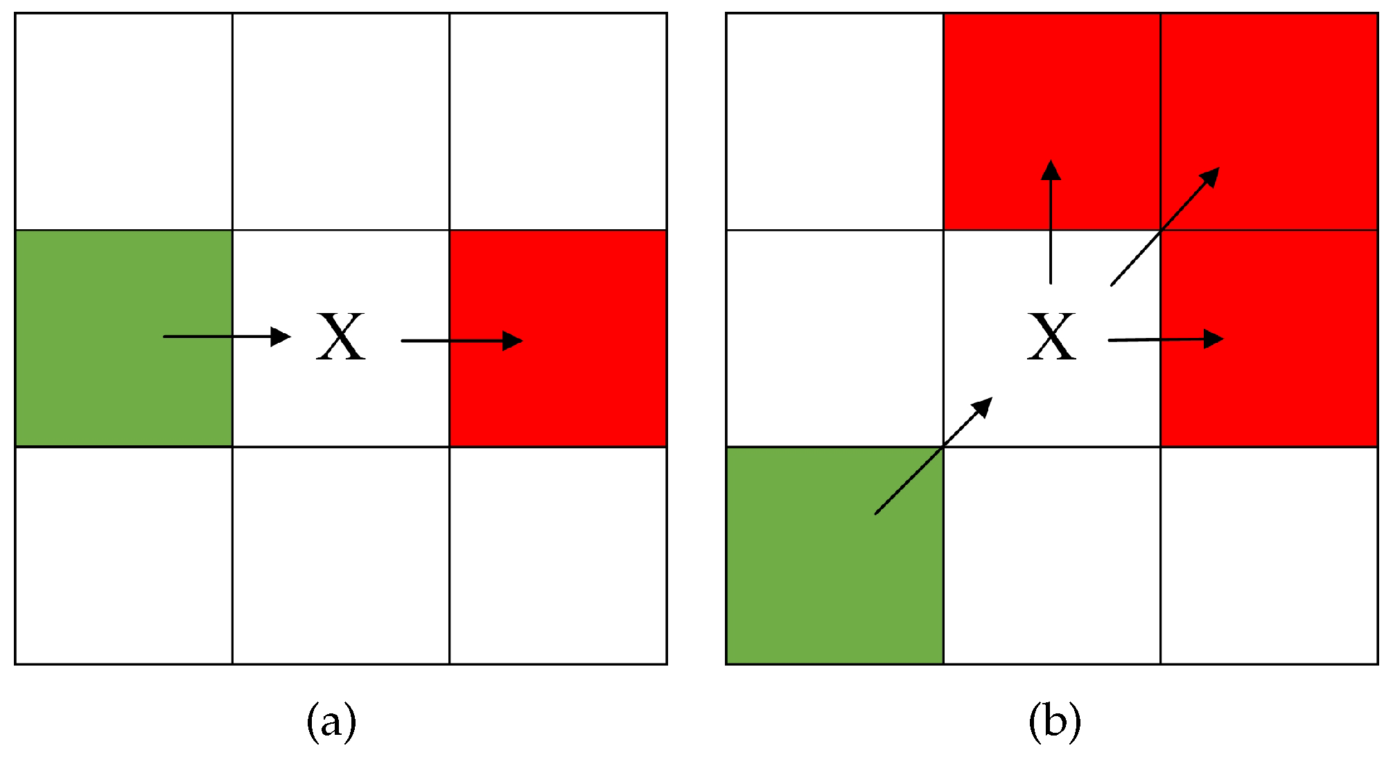
Figure 4.
Diagram of natural nodes. Green cells represent x’s parent node, and red cells represent x’s natural node. (a) Parent node in x’s horizontal or vertical direction. (b) Parent node in x’s diagonal direction.
Figure 4.
Diagram of natural nodes. Green cells represent x’s parent node, and red cells represent x’s natural node. (a) Parent node in x’s horizontal or vertical direction. (b) Parent node in x’s diagonal direction.
Figure 5.
Globalpath generation optimization flowchart. (a) Backtrack to detect the ancestor node that collides. (b) Search for the critical point that avoids collision. (c) Obtain the critical point C that avoids collision. (d) Obtain the critical point D that avoids collision. (e) Complete the path optimization.
Figure 6.
Kinematic model diagram of the robot, with positions before and after movement represented by ans , respectively.
Figure 6.
Kinematic model diagram of the robot, with positions before and after movement represented by ans , respectively.
Figure 7.
Diagram of the evaluation function, where is the angular difference between the robot’s orientation at the predicted endpoint and the target direction, and is the minimum distance between the robot’s position at the predicted endpoint and the obstacle.
Figure 7.
Diagram of the evaluation function, where is the angular difference between the robot’s orientation at the predicted endpoint and the target direction, and is the minimum distance between the robot’s position at the predicted endpoint and the obstacle.
Figure 8.
Diagram of deviation distance.
Figure 8.
Diagram of deviation distance.
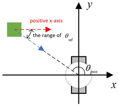
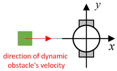
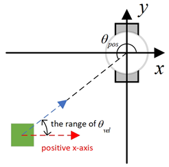
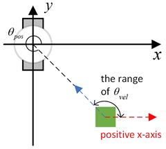
Figure 9.
Diagram of and , with the geometric center of the mobile robot set as the coordinate origin and the direction of the mobile robot’s velocity set as the positive x-axis.
Figure 9.
Diagram of and , with the geometric center of the mobile robot set as the coordinate origin and the direction of the mobile robot’s velocity set as the positive x-axis.
Figure 10.
Diagram of inflation radius: in the diagram, the inflation radius is 1.5 units, and the inflated space is depicted in yellow cells.
Figure 10.
Diagram of inflation radius: in the diagram, the inflation radius is 1.5 units, and the inflated space is depicted in yellow cells.
Figure 11.
Flowchart of the improved fusion path-planning algorithm. After the mobile robot completes map acquisition and processing, it executes the improved global path-planning algorithm to generate local path points. The robot starts from the starting point, continuously treats the next local path point as the current target, and eventually reaches the endpoint.
Figure 12.
Various global path-planning algorithms diagram for the 20 × 20 map environment, Zhang et al. proposed the improved JPS algorithm in reference [
22], written by Zhang et al. in 2021.
Figure 12.
Various global path-planning algorithms diagram for the 20 × 20 map environment, Zhang et al. proposed the improved JPS algorithm in reference [
22], written by Zhang et al. in 2021.
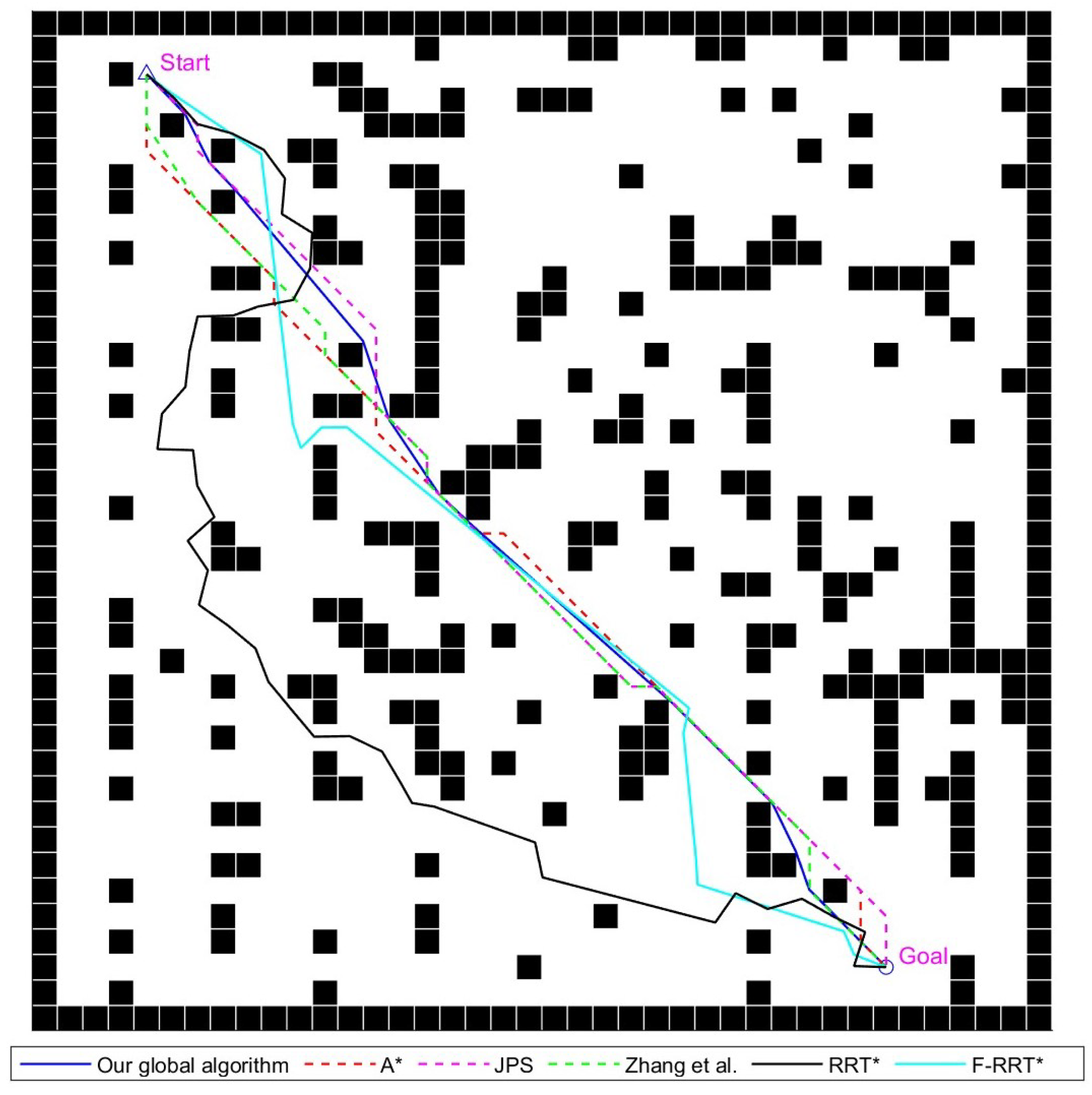
Figure 13.
Various global path-planning algorithms diagram for the 40 × 40 map environment, Zhang et al. proposed the improved JPS algorithm in reference [
22], written by Zhang et al. in 2021.
Figure 13.
Various global path-planning algorithms diagram for the 40 × 40 map environment, Zhang et al. proposed the improved JPS algorithm in reference [
22], written by Zhang et al. in 2021.
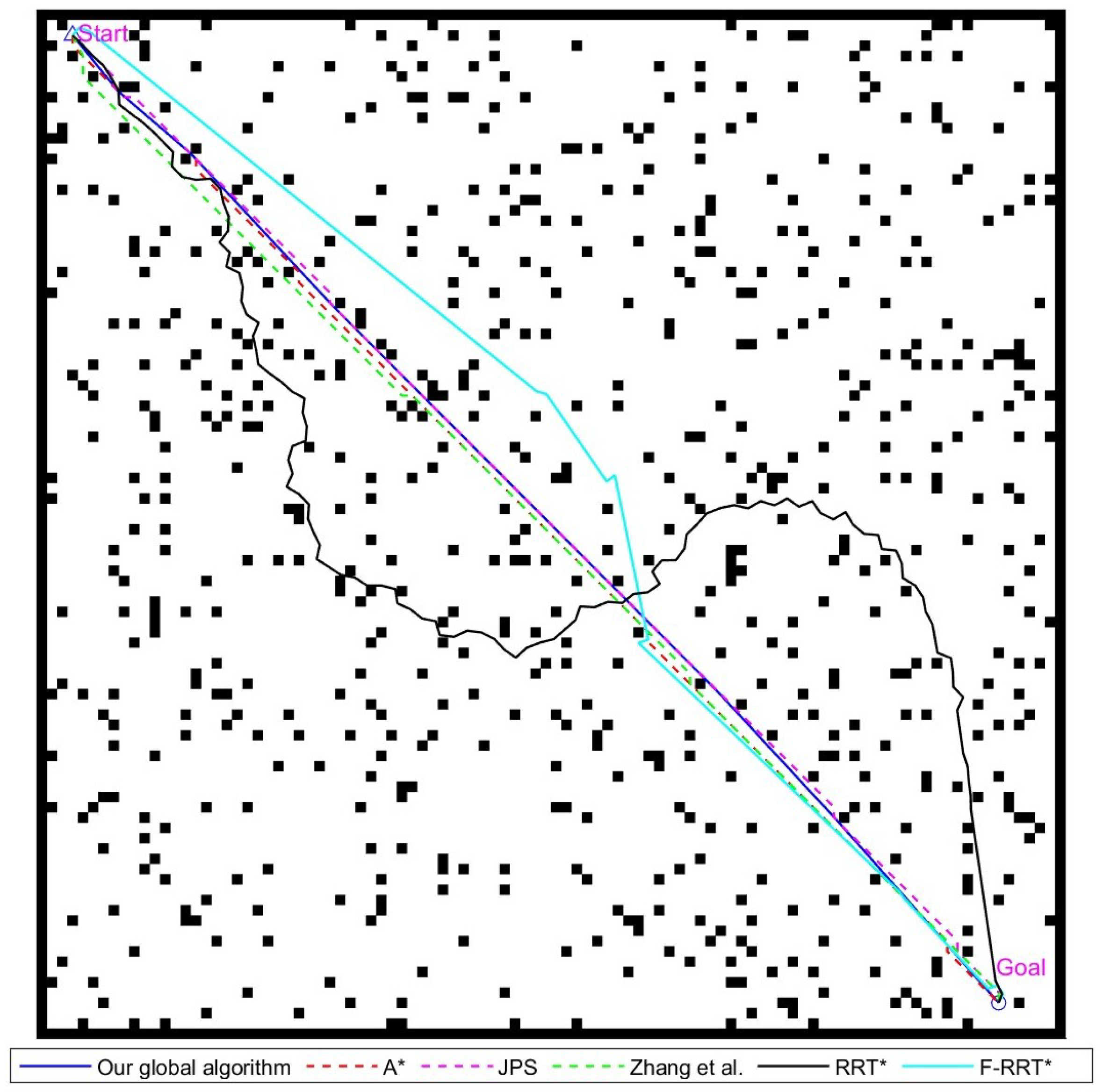
Figure 14.
Various global path-planning algorithms diagram for the 100 × 100 map environment, Zhang et al. proposed the improved JPS algorithm in reference [
22], written by Zhang et al. in 2021.
Figure 14.
Various global path-planning algorithms diagram for the 100 × 100 map environment, Zhang et al. proposed the improved JPS algorithm in reference [
22], written by Zhang et al. in 2021.
Figure 15.
Diagrams of an experiment for static scene 1, with yellow cells representing the inflated space, Zhang et al. proposed the improved JPS algorithm in reference [
22], written by Zhang et al. in 2021. (
a) Paths generated by various global path-planning algorithms. (
b) Paths traveled by the mobile robot using various fusion path-planning algorithms.
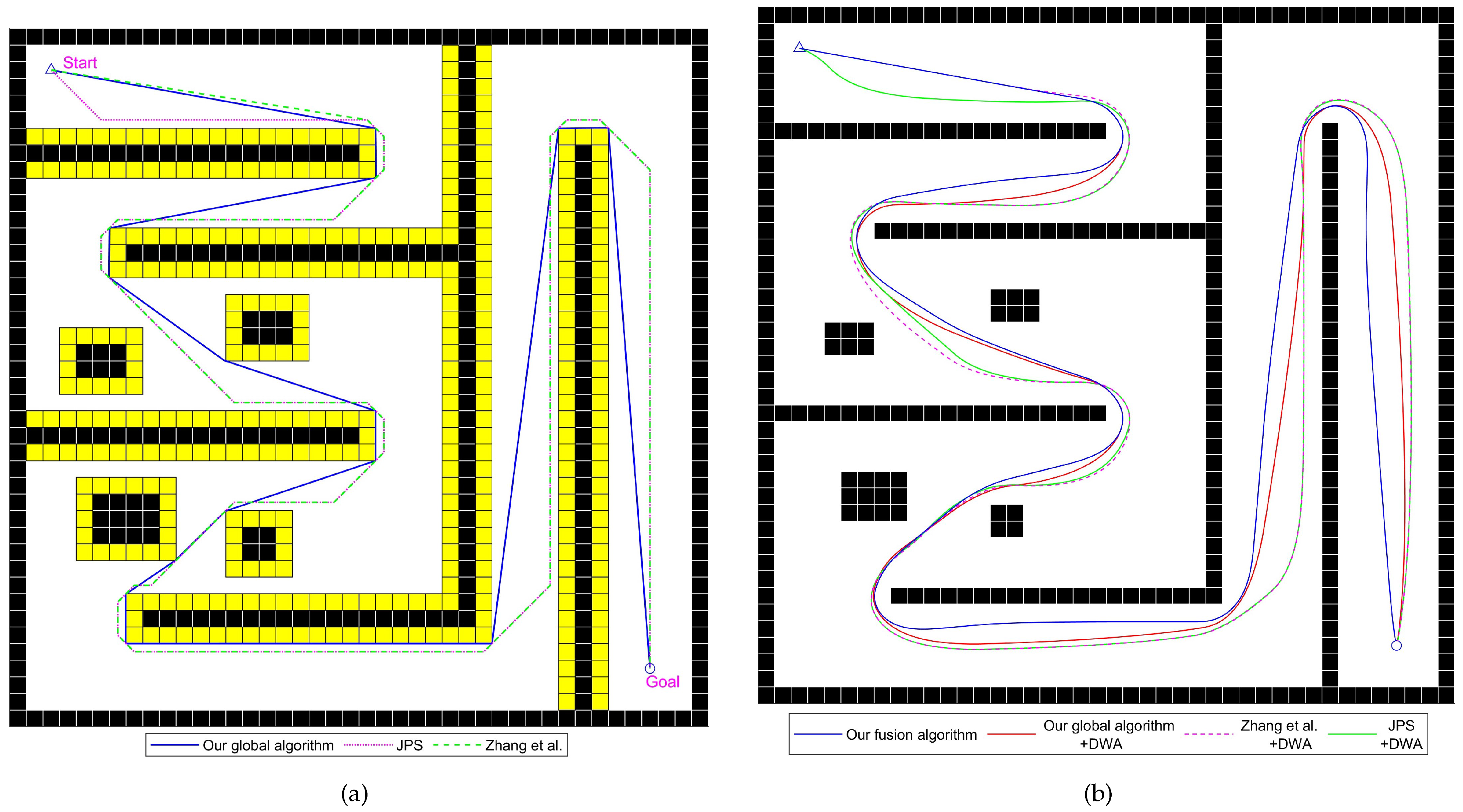
Figure 16.
Diagrams of the experiment for static scene 2, with yellow cells representing the inflated space, Zhang et al. proposed the improved JPS algorithm in reference [
22], written by Zhang et al. in 2021. (
a) Paths generated by various global path-planning algorithms. (
b) Paths traveled by the mobile robot using various fusion path-planning algorithms.
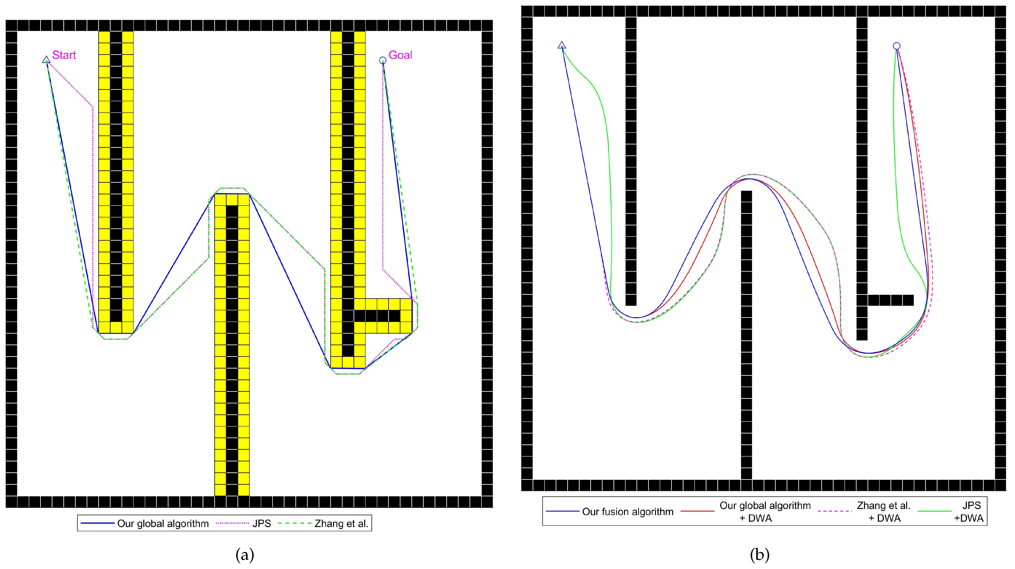
Figure 17.
Diagrams of the experiment for static scene 3, with yellow cells representing the inflated space, Zhang et al. proposed the improved JPS algorithm in reference [
22], written by Zhang et al. in 2021. (
a) Paths generated by various global path-planning algorithms. (
b) Paths traveled by the mobile robot using various fusion path-planning algorithms.
Figure 18.
Diagrams of the experiment for the static scene with unknown obstacles, with gray cells representing the unknown space. (a) The blue path is the route planned by our improved global path-planning algorithm, with yellow cells representing the inflated space. (b) Paths planned by the mobile robot using the DWA algorithm and our improved local path-planning algorithm.
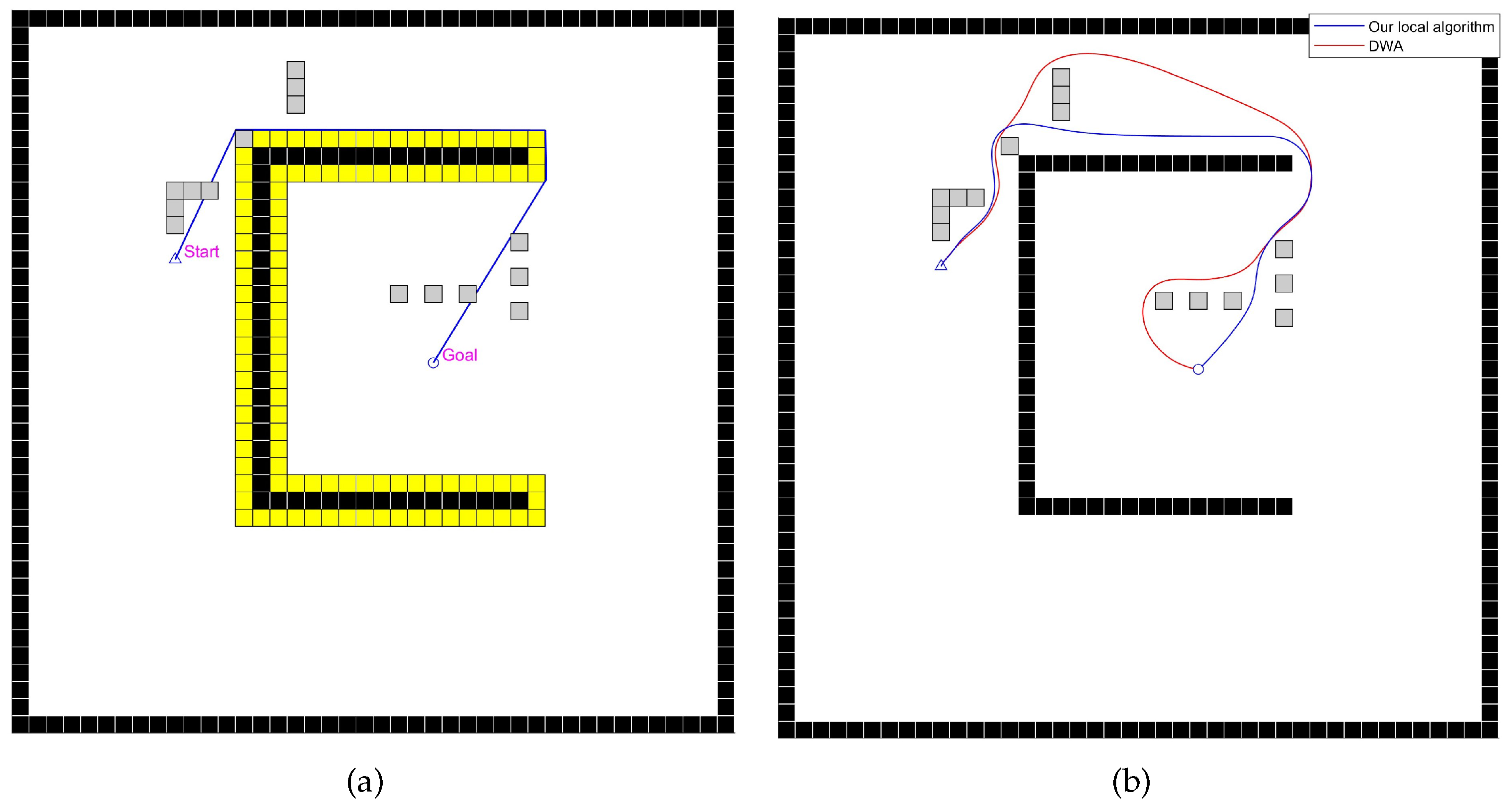
Figure 19.
Diagrams of the experiment for dynamic scene. (a) The blue and red paths respectively represent the planned paths of the mobile robot and the dynamic obstacle, with yellow cells representing the inflated space. (b) Diagram of the moment when the device using our improved local path-planning algorithm is closest to the dynamic obstacle, where the green rectangle represents the dynamic obstacle, and the black circle represents the mobile robot. The blue line represents the route that the robot has already traveled. (c) Diagram of the moment when the device using the DWA algorithm is closest to the dynamic obstacle. The blue line represents the route that the robot has already traveled. (d) Travel paths of the two fusion algorithms.
Table 1.
The relationship between and in various collision risk scenes.
Table 2.
Experimental results for global path-planning algorithms in the 20 × 20 map environment; the best results are highlighted.
Table 2.
Experimental results for global path-planning algorithms in the 20 × 20 map environment; the best results are highlighted.
| Global Algorithm | Calculation Time (ms) | Path Length | Number of Nodes | Total Turning Angle (°) |
|---|
| A* | 32 | 22.97 | 19 | 315 |
| JPS | 22 | 22.97 | 18 | 450 |
| Zhang et al. [22] | 23 | 22.24 | 8 | 180 |
| RRT* | 44 | 27.4 | 21 | 868° |
| F-RRT* | 84 | 22.41 | 12 | 510° |
| Our global algorithm | 23 | 21.71 | 7 | 59.38 |
Table 3.
Experimental results for global path-planning algorithms in the 40 × 40 map environment; the best results are highlighted.
Table 3.
Experimental results for global path-planning algorithms in the 40 × 40 map environment; the best results are highlighted.
| Global Algorithm | Calculation Time (ms) | Path Length | Number of Nodes | Total Turning Angle (°) |
|---|
| A* | 79 | 47.59 | 37 | 405° |
| JPS | 34 | 47.59 | 31 | 405° |
| Zhang et al. [22] | 35 | 47.37 | 12 | 405° |
| RRT* | 315 | 65.71 | 49 | 1753° |
| F-RRT* | 723 | 51.9 | 14 | 510° |
| Our global algorithm | 35 | 46.09 | 12 | 143.26° |
Table 4.
Experimental results for global path-planning algorithms in the 100 × 100 map environment; the best results are highlighted.
Table 4.
Experimental results for global path-planning algorithms in the 100 × 100 map environment; the best results are highlighted.
| Global Algorithm | Calculation Time (ms) | Path Length | Number of Nodes | Total Turning Angle (°) |
|---|
| A* | 121 | 131.86 | 96 | 495° |
| JPS | 44 | 131.86 | 83 | 495° |
| Zhang et al. [22] | 45 | 131.68 | 9 | 296.57° |
| RRT* | 2180 | 185.73 | 134 | 4113.69° |
| F-RRT* | 3260 | 138.19 | 15 | 778.59° |
| Our global algorithm | 48 | 130.23 | 7 | 21.89° |
Table 5.
Comparison of experimental results for static scene 1; the best results are highlighted.
Table 5.
Comparison of experimental results for static scene 1; the best results are highlighted.
| Fusion Algorithm | Global Path Length | Global Path Turning Angle (°) | Robot Travel Length | Robot
Travel Time (s) | Average Linear Velocity | Average Angular Velocity |
|---|
| JPS + DWA | 98.59 | 765 | 94.86 | 162.79 | 0.582 | 4.45 |
| Zhang et al. [22] + DWA | 96.00 | 538.26 | 94.25 | 161.49 | 0.583 | 3.42 |
| Our global algorithm + DWA | 92.01 | 425.57 | 90.57 | 155.29 | 0.583 | 3.03 |
| Our fusion algorithm | 92.01 | 425.57 | 90.34 | 153.67
| 0.587 | 2.93 |
Table 6.
Comparison of experimental results for static scene 2; the best results are highlighted.
Table 6.
Comparison of experimental results for static scene 2; the best results are highlighted.
| Fusion Algorithm | Global Path Length | Global Path Turning Angle (°) | Robot Travel Length | Robot
Travel Time (s) | Average Linear Velocity | Average Angular Velocity |
|---|
| JPS + DWA | 181.49 | 1125 | 176.58 | 297.08 | 0.594 | 3.79 |
| Zhang et al. [22] + DWA | 180.49 | 1071.03 | 176.88 | 296.28 | 0.597 | 3.5 |
| Our global algorithm + DWA | 172.4 | 886.29 | 169.13 | 282.98 | 0.597 | 3.33 |
| Our fusion algorithm | 172.4 | 886.29 | 167.5 | 278.96 | 0.600 | 3.32 |
Table 7.
Comparison of experimental results for static scene 3; the best results are highlighted.
Table 7.
Comparison of experimental results for static scene 3; the best results are highlighted.
| Fusion Algorithm | Global Path Length | Global Path Turning Angle (°) | Robot Travel Length | Robot
Travel Time (s) | Average Linear Velocity | Average Angular Velocity |
|---|
| JPS + DWA | 288.04 | 1035 | 283.34 | 443.56 | 0.606 | 2.35 |
| Zhang et al. [22] + DWA | 284.22 | 889.7 | 280.75 | 462.87 | 0.606 | 1.94 |
| Our global algorithm + DWA | 272.91 | 606.9 | 270.61 | 445.27 | 0.607 | 1.53 |
| Our fusion algorithm | 272.91 | 606.9 | 270.45 | 443.57 | 0.610 | 1.45 |
Table 8.
Comparison of experimental results for the static scene with unknown obstacles; the best results are highlighted.
Table 8.
Comparison of experimental results for the static scene with unknown obstacles; the best results are highlighted.
| Local Algorithm | Robot Travel Length | Robot Travel Time (s) | Average Linear Velocity | Average Angular Velocity |
|---|
| DWA | 51.31 | 92.82 | 0.552 | 6.46 |
| Our local algorithm | 42.12 | 76.21 | 0.552 | 5.75 |
Table 9.
Comparison of experimental results for the dynamic scene, where “Closest distance” refers to the minimum distance between the robot and the dynamic obstacle during its journey.
Table 9.
Comparison of experimental results for the dynamic scene, where “Closest distance” refers to the minimum distance between the robot and the dynamic obstacle during its journey.
| Local Algorithm | Robot Travel Length | Robot Travel Time (s) | Average Linear Velocity | Average Angular Velocity | Closest Distance |
|---|
| DWA | 47.66 | 84.51 | 0.566 | 0.457 | 0.62 |
| Our local algorithm | 47.75 | 84.08 | 0.567 | 0.968 | 1.27 |


