
YOLO-DHGC: Small Object Detection Using Two-Stream Structure with Dense Connections


Abstract

1. Introduction
- (1)
- We designed a two-stream structure based on an edge-gated branch, which includes a regular detection stream and an edge-gated stream. The regular detection stream uses the DenseHRNet backbone to capture high-level semantic information from the image. An edge-gated stream is especially proposed to extract object contour information of small objects in images with complex backgrounds. The localization accuracy of small objects is improved by emphasizing boundary information and reducing background interference;
- (2)
- We designed a feature extraction backbone network called DenseHRNet. By incorporating a dense connection mechanism, the network extracts and transmits feature information across multiple layers in the main pathway of high-resolution feature maps. This proposed mechanism compensates the loss of the detailed information of objects, which occurs due to reduced image resolution after downsampling. As the backbone of the regular detection stream, DenseHRNet uses a dense connection mechanism to transmit feature information across multiple layers, thereby improving the accuracy of small object recognition;
- (3)
- To further verify the performance of our method, we constructed a dataset of backlight panel images with surface micro-defects captured in a real industrial production line. This dataset was used to test and validate the generalization performance of the YOLO-DHGC algorithm.
2. Related Work
2.1. Small Object Detection
2.2. Two-Stream Structure in Spatial and Temporal Feature Extraction
2.3. Dense Connections for Feature Reuse
3. Methods
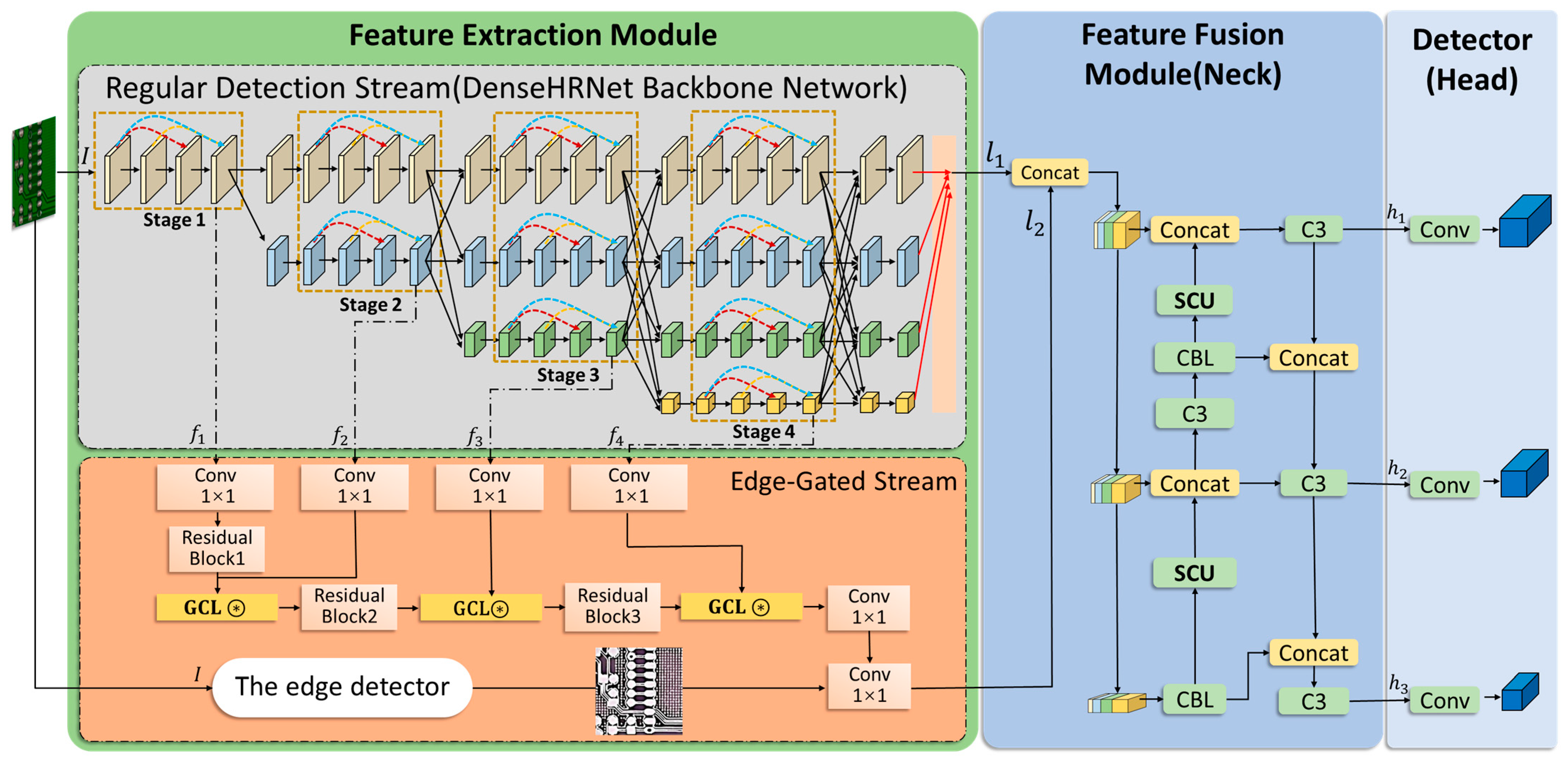
3.1. YOLO-DHGC
3.2. Feature Extraction Module
3.2.1. Regular Detection Stream with DenseHRNet Backbone Network
3.2.2. Edge-Gated Stream
3.2.3. Two-Stream Object Detection Structure Based on Edge-Gated Branch
3.3. Feature Fusion Module
3.4. Object Detection Heads
4. Experiments
4.1. Dataset
4.1.1. PKU-Market-PCB Dataset
4.1.2. NEU-DET Hot Rolled Steel Surface Defect Dataset
4.1.3. TinyPerson Dataset
4.1.4. Self-Constructed Backlight Panel Micro-Defect Dataset
4.2. Assessment of Indicators
4.3. Experimental Configurations
4.4. Benchmark Selection Comparison Experiment
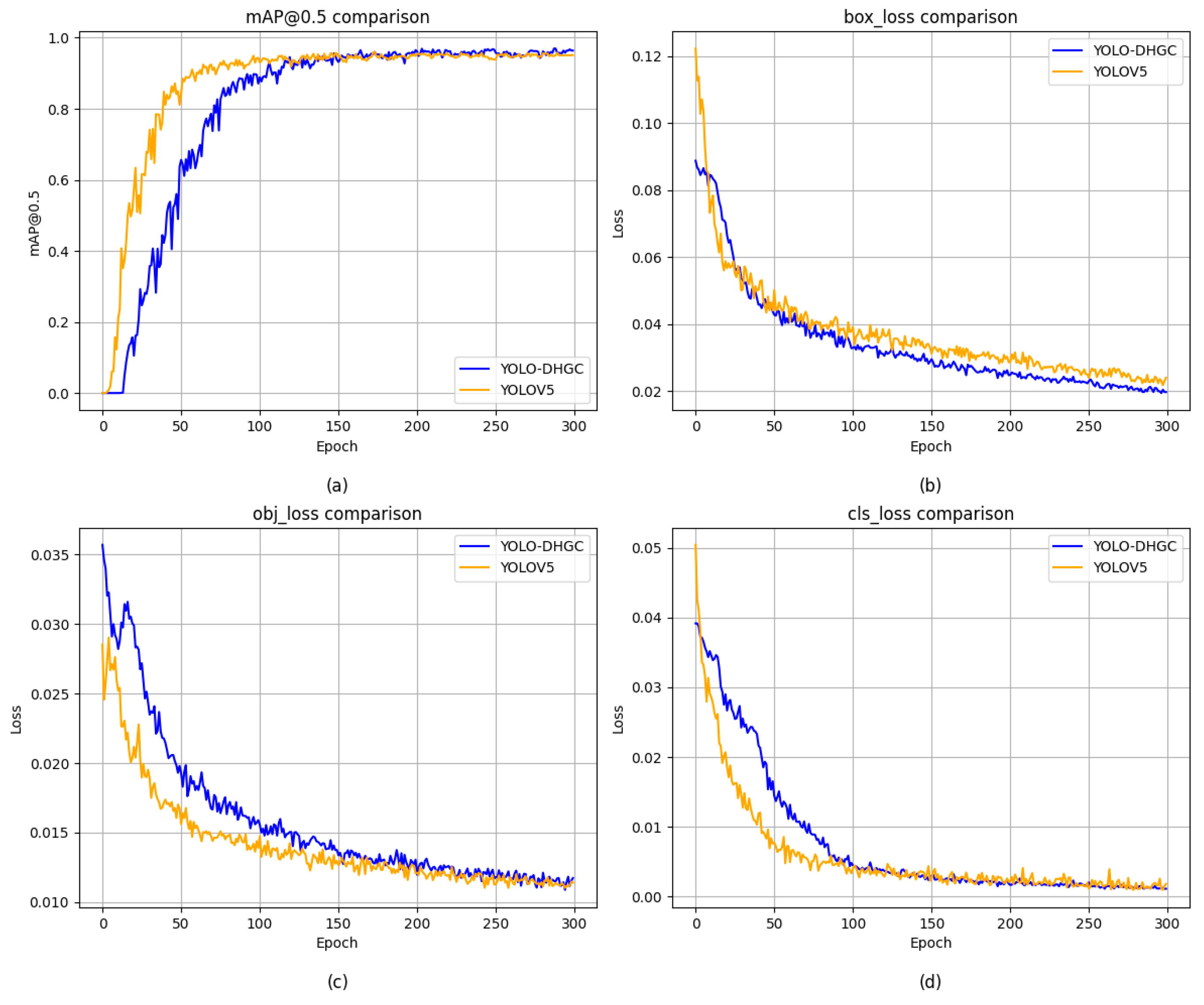
4.5. Model Training
4.6. Experimental Results
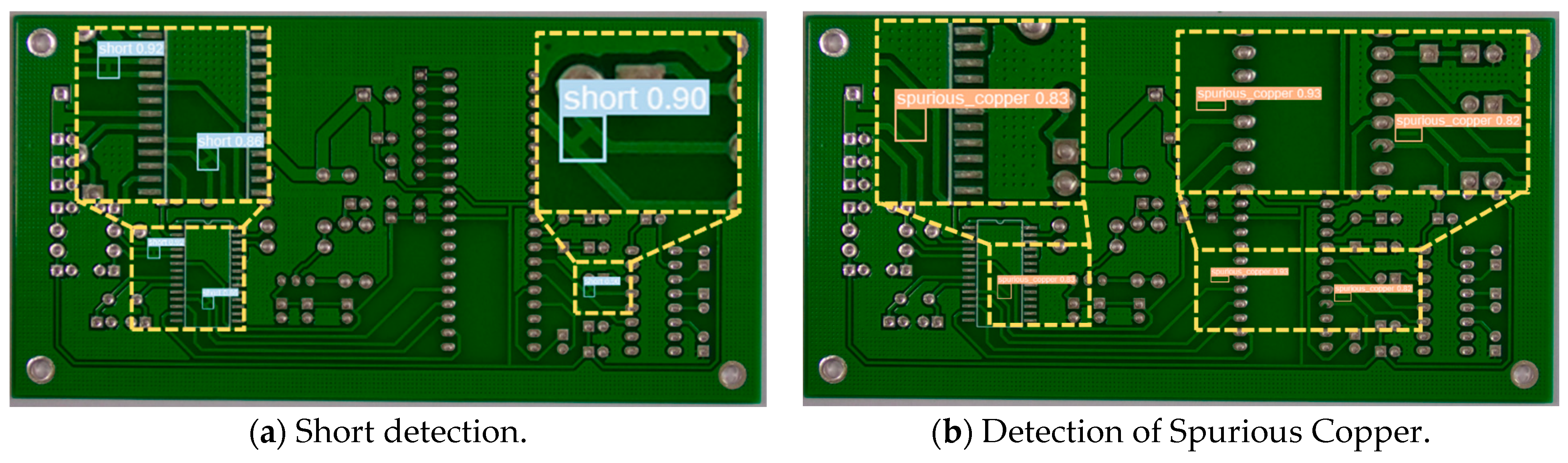
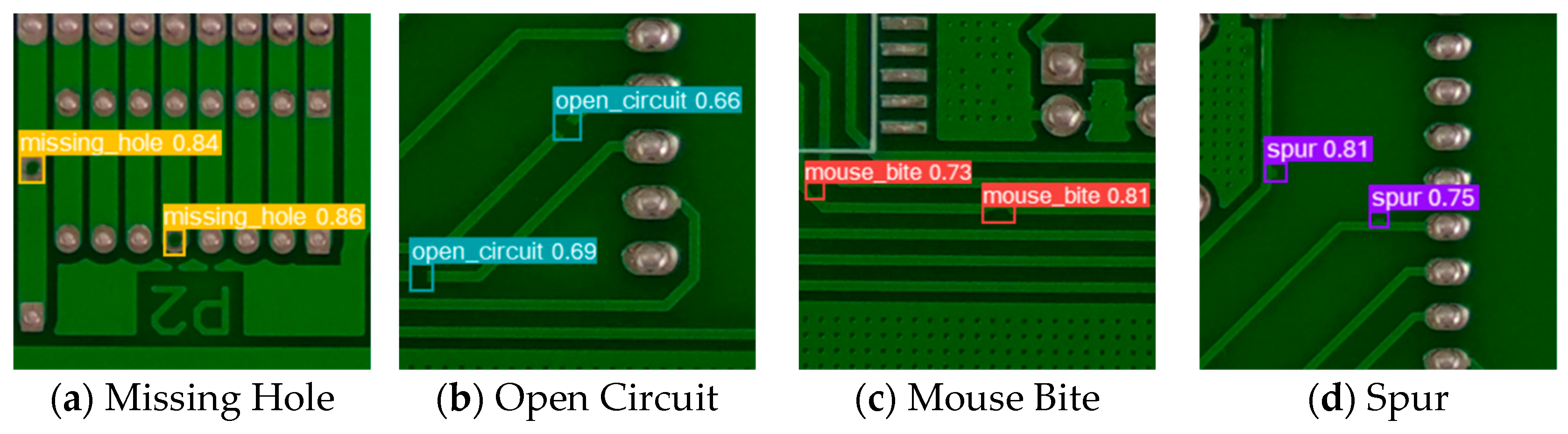
4.6.1. PKU-Market-PCB Dataset
4.6.2. Analysis of Experimental Results of NEU-DET Hot-Rolled Steel Surface Defect Dataset
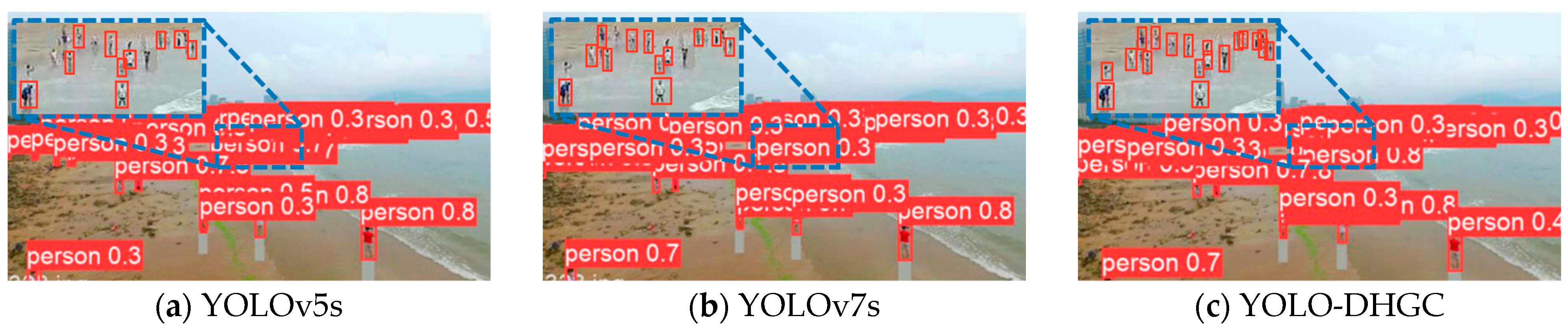
4.6.3. Analysis of Experimental Results on TinyPerson Dataset
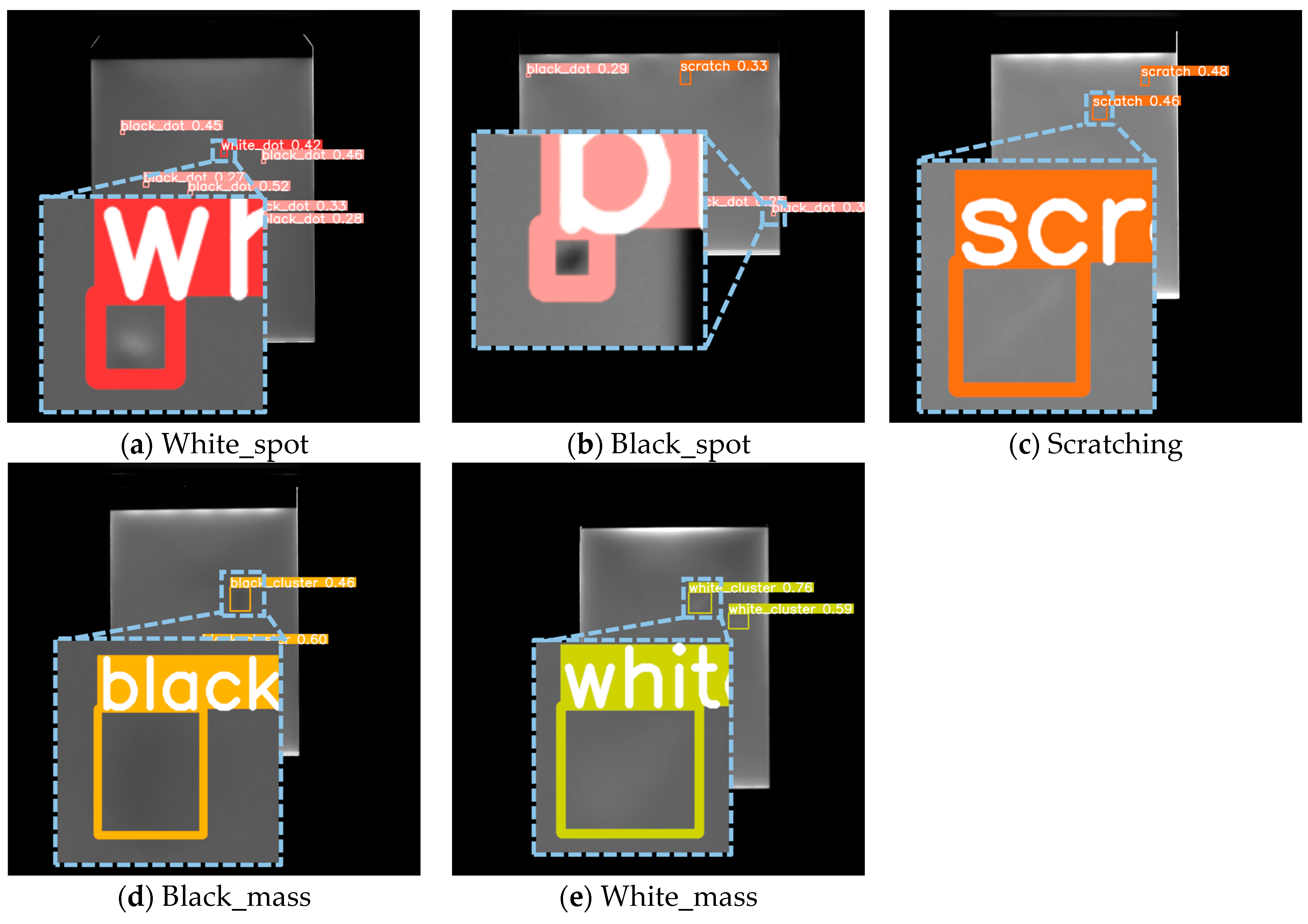
4.6.4. Self-Constructed Backlight Panel Micro-Defect Dataset
4.7. Ablation Experiments
- Utilization of the DenseHRNet Backbone
- Two-stream Object Detection Structure Based on the Edge-Gated Branch
- Using Both the DenseHRNet Backbone and the Edge-Gated Two-stream Detection Structure
5. Conclusions
Author Contributions
Funding
Data Availability Statement
Acknowledgments
Conflicts of Interest
References
- Qiu, Z.; Wang, S.; Zeng, Z.; Yu, D. Automatic visual defects inspection of wind turbine blades via YOLO-based small object detection approach. J. Electron. Imaging 2019, 28, 043023. [Google Scholar] [CrossRef]
- Spencer Jr, B.F.; Hoskere, V.; Narazaki, Y. Advances in computer vision-based civil infrastructure inspection and monitoring. Engineering 2019, 5, 199–222. [Google Scholar] [CrossRef]
- Tulbure, A.-A.; Tulbure, A.-A.; Dulf, E.-H. A review on modern defect detection models using DCNNs–Deep convolutional neural networks. J. Adv. Res. 2022, 35, 33–48. [Google Scholar] [CrossRef] [PubMed]
- Zou, Z.; Chen, K.; Shi, Z.; Guo, Y.; Ye, J. Object detection in 20 years: A survey. Proc. IEEE 2023, 111, 257–276. [Google Scholar] [CrossRef]
- Girshick, R.; Donahue, J.; Darrell, T.; Malik, J. Rich feature hierarchies for accurate object detection and semantic segmentation. In Proceedings of the IEEE Conference on Computer Vision and Pattern Recognition, Columbus, OH, USA, 23–28 June 2014; pp. 580–587. [Google Scholar]
- Girshick, R. Fast r-cnn. In Proceedings of the IEEE International Conference on Computer Vision, Santiago, Chile, 7–13 December 2015; pp. 1440–1448. [Google Scholar]
- Ren, S.; He, K.; Girshick, R.; Sun, J. Faster r-cnn: Towards real-time object detection with region proposal networks. In Proceedings of the Advances in Neural Information Processing Systems (NIPS 2015), Montreal, QC, Canada, 7–13 December 2015; Volume 28. [Google Scholar]
- Kisantal, M.; Wojna, Z.; Murawski, J.; Naruniec, J.; Cho, K. Augmentation for small object detection. arXiv 2019, arXiv:1902.07296. [Google Scholar]
- Huang, Y.; Fan, J.; Hu, Y.; Guo, J.; Zhu, Y. TBi-YOLOv5: A surface defect detection model for crane wire with Bottleneck Transformer and small object detection layer. Proc. Inst. Mech. Eng. Part C J. Mech. Eng. Sci. 2024, 238, 2425–2438. [Google Scholar] [CrossRef]
- Zoph, B.; Cubuk, E.D.; Ghiasi, G.; Lin, T.-Y.; Shlens, J.; Le, Q.V. Learning data augmentation strategies for object detection. In Proceedings of the Computer Vision–ECCV 2020: 16th European Conference, Glasgow, UK, 23–28 August 2020; Proceedings, Part XXVII 16. Springer International Publishing: Berlin/Heidelberg, Germany, 2020; pp. 566–583. [Google Scholar]
- Lin, T.-Y.; Dollár, P.; Girshick, R.; He, K.; Hariharan, B.; Belongie, S. Feature pyramid networks for object detection. In Proceedings of the IEEE Conference on Computer Vision and Pattern Recognition, Honolulu, HI, USA, 21–26 July 2017; pp. 2117–2125. [Google Scholar]
- Zeng, N.; Wu, P.; Wang, Z.; Li, H.; Liu, W.; Liu, X. A small-sized object detection oriented multi-scale feature fusion approach with application to defect detection. IEEE Trans. Instrum. Meas. 2022, 71, 1–14. [Google Scholar] [CrossRef]
- Luo, P.; Wang, B.; Wang, H.; Ma, F.; Ma, H.; Wang, L. An ultrasmall bolt defect detection method for transmission line inspection. IEEE Trans. Instrum. Meas. 2023, 72, 1–12. [Google Scholar] [CrossRef]
- Xiao, J.; Zhao, T.; Yao, Y.; Yu, Q.; Chen, Y. Context Augmentation and Feature Refinement Network for Tiny Object Detection. Available online: https://openreview.net/pdf?id=q2ZaVU6bEsT (accessed on 15 September 2024).
- Luo, H.-W.; Zhang, C.-S.; Pan, F.-C.; Ju, X.-M. Contextual-YOLOV3: Implement better small object detection based deep learning. In Proceedings of the 2019 International Conference on Machine Learning, Big Data and Business Intelligence (MLBDBI), Taiyuan, China, 8–10 November 2019; pp. 134–141. [Google Scholar]
- Fu, K.; Li, J.; Ma, L.; Mu, K.; Tian, Y. Intrinsic relationship reasoning for small object detection. arXiv 2020, arXiv:2009.00833. [Google Scholar]
- Zhong, Y.; Wang, J.; Peng, J.; Zhang, L. Anchor box optimization for object detection. In Proceedings of the IEEE/CVF Winter Conference on Applications of Computer Vision, Seattle, WA, USA, 13–19 June 2020; pp. 1286–1294. [Google Scholar]
- Kong, T.; Sun, F.; Liu, H.; Jiang, Y.; Li, L.; Shi, J. Foveabox: Beyound anchor-based object detection. IEEE Trans. Image Process. 2020, 29, 7389–7398. [Google Scholar] [CrossRef]
- Zhang, Y.; Zhang, H.; Huang, Q.; Han, Y.; Zhao, M. DsP-YOLO: An anchor-free network with DsPAN for small object detection of multiscale defects. Expert Syst. Appl. 2024, 241, 122669. [Google Scholar] [CrossRef]
- Bosquet, B.; Cores, D.; Seidenari, L.; Brea, V.M.; Mucientes, M.; Del Bimbo, A. A full data augmentation pipeline for small object detection based on generative adversarial networks. Pattern Recognit. 2023, 133, 108998. [Google Scholar] [CrossRef]
- Ji, S.-J.; Ling, Q.-H.; Han, F. An improved algorithm for small object detection based on YOLO v4 and multi-scale contextual information. Comput. Electr. Eng. 2023, 105, 108490. [Google Scholar] [CrossRef]
- Li, J.; Liang, X.; Wei, Y.; Xu, T.; Feng, J.; Yan, S. Perceptual generative adversarial networks for small object detection. In Proceedings of the IEEE Conference on Computer Vision and Pattern Recognition, Honolulu, HI, USA, 21–26 July 2017; pp. 1222–1230. [Google Scholar]
- Yang, T.; Wang, S.; Tong, J.; Wang, W. Accurate real-time obstacle detection of coal mine driverless electric locomotive based on ODEL-YOLOv5s. Sci. Rep. 2023, 13, 17441. [Google Scholar] [CrossRef] [PubMed]
- Tong, X.; Su, S.; Wu, P.; Guo, R.; Wei, J.; Zuo, Z.; Sun, B. MSAFFNet: A multiscale label-supervised attention feature fusion network for infrared small object detection. IEEE Trans. Geosci. Remote Sens. 2023, 61, 1–16. [Google Scholar] [CrossRef]
- Tang, S.; Zhang, S.; Fang, Y. HIC-YOLOv5: Improved YOLOv5 for small object detection. In Proceedings of the 2024 IEEE International Conference on Robotics and Automation (ICRA), Yokohama, Japan, 13–17 May 2024; pp. 6614–6619. [Google Scholar]
- Zhang, T.; Li, L.; Cao, S.; Pu, T.; Peng, Z. Attention-guided pyramid context networks for detecting infrared small object under complex background. IEEE Trans. Aerosp. Electron. Syst. 2023, 59, 4250–4261. [Google Scholar] [CrossRef]
- Dai, Y.; Li, X.; Zhou, F.; Qian, Y.; Chen, Y.; Yang, J. One-stage cascade refinement networks for infrared small object detection. IEEE Trans. Geosci. Remote Sens. 2023, 61, 1–17. [Google Scholar]
- Simonyan, K.; Zisserman, A. Two-stream convolutional networks for action recognition in videos. In Proceedings of the Advances in Neural Information Processing Systems 27 (NIPS 2014), Montreal, QC, Canada, 8–13 December 2014; Volume 27. [Google Scholar]
- Li, B.; Cui, W.; Wang, W.; Zhang, L.; Chen, Z.; Wu, M. Two-stream convolution augmented transformer for human activity recognition. In Proceedings of the AAAI Conference on Artificial Intelligence, Virtually, 2–9 February 2021; pp. 286–293. [Google Scholar]
- Cheng, X.; Zhang, M.; Lin, S.; Zhou, K.; Zhao, S.; Wang, H. Two-stream isolation forest based on deep features for hyperspectral anomaly detection. IEEE Geosci. Remote Sens. Lett. 2023, 20, 1–5. [Google Scholar] [CrossRef]
- Yi, Y.; Zhang, N.; Zhou, W.; Shi, Y.; Xie, G.; Wang, J. GPONet: A two-stream gated progressive optimization network for salient object detection. Pattern Recognit. 2024, 150, 110330. [Google Scholar] [CrossRef]
- Huang, G.; Liu, Z.; Van Der Maaten, L.; Weinberger, K.Q. Densely connected convolutional networks. In Proceedings of the IEEE Conference on Computer Vision and Pattern Recognition, Honolulu, HI, USA, 21–26 July 2017; pp. 4700–4708. [Google Scholar]
- Fang, S.; Li, K.; Shao, J.; Li, Z. SNUNet-CD: A densely connected Siamese network for change detection of VHR images. IEEE Geosci. Remote Sens. Lett. 2021, 19, 1–5. [Google Scholar] [CrossRef]
- Zhang, J.; Zhang, Y.; Jin, Y.; Xu, J.; Xu, X. Mdu-net: Multi-scale densely connected u-net for biomedical image segmentation. Health Inf. Sci. Syst. 2023, 11, 13. [Google Scholar] [CrossRef] [PubMed]
- Ju, R.-Y.; Chen, C.-C.; Chiang, J.-S.; Lin, Y.-S.; Chen, W.-H. Resolution enhancement processing on low quality images using swin transformer based on interval dense connection strategy. Multimed. Tools Appl. 2024, 83, 14839–14855. [Google Scholar] [CrossRef]
- Wang, J.; Sun, K.; Cheng, T.; Jiang, B.; Deng, C.; Zhao, Y.; Liu, D.; Mu, Y.; Tan, M.; Wang, X. Deep high-resolution representation learning for visual recognition. IEEE Trans. Pattern Anal. Mach. Intell. 2020, 43, 3349–3364. [Google Scholar] [CrossRef] [PubMed]
- Iandola, F. Densenet: Implementing Efficient Convnet Descriptor Pyramids. arXiv 2014, arXiv:1404.1869. [Google Scholar]


| Number of Labels/Images | Training Set | Validation Set | Test Set | Totals | ||
|---|---|---|---|---|---|---|
| Original | Enhancement | Original | Enhancement | |||
| Missing Hole | 340 | 1987 | 53 | 56 | 449 | 2327 |
| Mouse Bite | 314 | 1804 | 49 | 48 | 411 | 2118 |
| Open Circuit | 358 | 2058 | 50 | 45 | 453 | 2416 |
| Short | 340 | 1998 | 40 | 53 | 433 | 2338 |
| Spur | 385 | 2258 | 47 | 41 | 473 | 2643 |
| Spurious Copper | 351 | 2078 | 51 | 41 | 443 | 2429 |
| Total Number of Images | 555 | 3330 | 69 | 69 | 693 | 3885 |
| Number of Labels/Images | Training Set | Validation Set | Test Set | Totals |
|---|---|---|---|---|
| Crazing, Cr | 532 | 74 | 83 | 689 |
| Inclusion, In | 732 | 80 | 69 | 881 |
| Patches, Pa | 784 | 116 | 112 | 1012 |
| Pitted Surface, Ps | 327 | 47 | 58 | 432 |
| Rolled-in Scale, Rs | 505 | 68 | 55 | 628 |
| Scratches, Sc | 408 | 65 | 75 | 548 |
| Total Number of Images | 1440 | 180 | 180 | 1800 |
| Number of Images or Labels | Training Set | Validation Set | Totals |
|---|---|---|---|
| Number of Images | 794 | 816 | 1610 |
| Number of Labels | 42,197 | 30,454 | 72,651 |
| Number of Defects/Images | Training Set | Validation Set | Test Set | Totals | ||
|---|---|---|---|---|---|---|
| Original | Enhancement | Original | Enhancement | |||
| White_spot | 107 | 1562 | 28 | 24 | 159 | 1614 |
| Black_spot | 541 | 7259 | 42 | 44 | 627 | 7345 |
| Scratching | 89 | 1280 | 20 | 19 | 128 | 1319 |
| Black_mass | 45 | 628 | 15 | 13 | 73 | 656 |
| White_mass | 84 | 1202 | 18 | 19 | 121 | 1239 |
| Total Number of Images | 241 | 3374 | 31 | 31 | 303 | 3436 |
| Detection Algorithms | Backbone Network | PCB | NEU-DET | ||||||
|---|---|---|---|---|---|---|---|---|---|
| mAP@0.5 (%) | APS (%) | APM (%) | APL (%) | mAP@0.5 (%) | APS (%) | APM (%) | APL (%) | ||
| YOLOv5s | Modified CSP v5 | 94.3 | 45.9 | 55.1 | 56.5 | 76.9 | 42.7 | 50.7 | 51.1 |
| YOLOv8s | CSPDarknet53 | 93.2 | 40.4 | 38.5 | 51.6 | 74.7 | 38.3 | 33.3 | 42.1 |
| Detection Algorithms | Backbone Network | mAP@0.5 (%) | mAP@0.75 (%) | mAP@0.5:0.95 (%) | APS (%) | APM (%) | APL (%) |
|---|---|---|---|---|---|---|---|
| Faster R-CNN | ResNet-101 | 90.5 | 41.0 | 50.1 | 42.7 | 50.7 | 51.1 |
| Cascade R-CNN | ResNet-101 | 91.8 | 42.6 | 50.5 | 44.9 | 53.1 | 53.8 |
| SSD512 | ResNet-101 | 780.5 | 36.5 | 44.3 | 37.6 | 42.8 | 46.9 |
| RetinaNet | ResNet-101 | 84.1 | 40.2 | 45.9 | 38.9 | 47.6 | 47.3 |
| YOLOv4 | CSPDarknet-53 | 92.7 | 44.7 | 51.8 | 44.8 | 53 | 53.1 |
| YOLOv5s | Modified CSP v5 | 94.3 | 47.8 | 52.6 | 45.9 | 55.1 | 56.5 |
| YOLOX-s | Modified CSP v5 | 92.9 | 45.7 | 51.5 | 45.1 | 53.4 | 52.9 |
| YOLOv7s | RepConvN | 95.8 | 48.2 | 53.3 | 46.6 | 55.2 | 56.3 |
| DETR | ResNet-50 | 91.2 | 44.4 | 49.2 | 23.3 | 46.7 | 46.5 |
| YOLO-DHGC (ours) | DHRNet-W32 | 96.3 | 48.5 | 54.0 | 48.5 | 55.4 | 56.9 |
| Detection Algorithms | Backbone Network | mAP@0.5(%) | |||||
|---|---|---|---|---|---|---|---|
| Missing Hole | Mouse Bite | Open Circuit | Short | Spur | Spurious Copper | ||
| Faster R-CNN | ResNet-101 | 93.9 | 91.8 | 88.3 | 92.6 | 83.7 | 92.6 |
| Cascade R-CNN | ResNet-101 | 94.6 | 93.7 | 90.1 | 94.2 | 86.7 | 91.8 |
| SSD512 | ResNet-101 | 91.6 | 84.6 | 78.3 | 85.5 | 76.3 | 80.5 |
| RetinaNet | ResNet-101 | 87.8 | 85.1 | 80.6 | 85.5 | 79.5 | 84.4 |
| YOLOv4 | CSPDarknet-53 | 95.3 | 93.2 | 92.3 | 94.1 | 85.4 | 93.8 |
| YOLOv5s | Modified CSP v5 | 96.4 | 94.9 | 92.1 | 95.9 | 90.7 | 95.5 |
| YOLOX-s | Modified CSP v5 | 94.1 | 93.6 | 90.4 | 93.8 | 88.6 | 94.1 |
| YOLOv7s | RepConvN | 99.1 | 96.7 | 94.9 | 98.6 | 91.5 | 94.6 |
| DETR | ResNet-50 | 92.7 | 91.7 | 89.9 | 92.8 | 86.7 | 93.1 |
| YOLO-DHGC (ours) | DHRNet-W32 | 99.3 | 97.4 | 95.9 | 97.2 | 91.8 | 96.1 |
| Detection Algorithms | Backbone Network | mAP@0.5 (%) | mAP@0.75 (%) | mAP@0.5:0.95 (%) | APS (%) | APM (%) | APL (%) |
|---|---|---|---|---|---|---|---|
| Faster R-CNN | ResNet-101 | 72.9 | 40.8 | 43.1 | 38.1 | 40.4 | 49.1 |
| Cascade R-CNN | ResNet-101 | 76.3 | 39.7 | 43.1 | 40.8 | 42.4 | 50.6 |
| SSD512 | ResNet-101 | 71 | 34.9 | 37.4 | 31.4 | 32.3 | 43.5 |
| RetinaNet | ResNet-101 | 72.5 | 38.8 | 40.8 | 35.5 | 37.7 | 44.2 |
| YOLOv4 | CSPDarknet-53 | 75.1 | 41 | 45.1 | 41.4 | 43.6 | 50.6 |
| YOLOv5s | Modified CSP v5 | 76.9 | 46.2 | 47.2 | 41.5 | 44.6 | 51.2 |
| YOLOX-s | Modified CSP v5 | 76.4 | 42.2 | 47.5 | 42.7 | 42.5 | 51.5 |
| YOLOv7s | RepConvN | 80.2 | 47.1 | 49.3 | 43.1 | 45.3 | 51.8 |
| YOLO-DHGC (ours) | DHRNet-W32 | 81.6 | 47.8 | 50.2 | 44.3 | 45.4 | 51.2 |
| Detection Algorithms | Backbone Network | mAP@0.5 (%) | |||||
|---|---|---|---|---|---|---|---|
| Cr | In | Pa | Ps | Rs | Sc | ||
| Faster R-CNN | ResNet-101 | 40.9 | 77.4 | 85.9 | 82.4 | 66.5 | 84.2 |
| Cascade R-CNN | ResNet-101 | 44.8 | 78.8 | 88.8 | 85.4 | 70.9 | 87.3 |
| SSD512 | ResNet-101 | 35.6 | 78.2 | 85.6 | 79.6 | 60.7 | 83.2 |
| RetinaNet | ResNet-101 | 39.8 | 75.3 | 84.7 | 80.6 | 68.2 | 84.5 |
| YOLOv4 | CSPDarknet-53 | 41.8 | 77.5 | 86.6 | 85.1 | 70.4 | 85.3 |
| YOLOv5s | Modified CSP v5 | 48.3 | 82.8 | 89.4 | 85.9 | 75.2 | 83.9 |
| YOLOX-s | Modified CSP v5 | 44.4 | 83.1 | 87.2 | 79.5 | 80.0 | 86.3 |
| YOLOv7s | RepConvN | 50.2 | 86.5 | 90.4 | 85.4 | 79.2 | 84.5 |
| YOLO-DHGC (ours) | DHRNet-W32 | 51.1 | 85.8 | 91.5 | 87.9 | 78.9 | 87.4 |
| Detection Algorithms | Backbone Network | (%) | (%) | (%) | (%) | (%) | (%) | (%) |
|---|---|---|---|---|---|---|---|---|
| Faster R-CNN | ResNet-101 | 48.01 | 29.45 | 50.25 | 57.69 | 63.29 | 69.32 | 6.03 |
| Cascade R-CNN | ResNet-101 | 51.12 | 31.78 | 53.21 | 60.38 | 65.12 | 72.01 | 6.42 |
| SSD512 | ResNet-101 | 34.12 | 13.48 | 35.29 | 48.83 | 57.36 | 61.67 | 2.67 |
| RetinaNet | ResNet-101 | 45.52 | 26.63 | 51.01 | 55.78 | 57.38 | 68.24 | 4.16 |
| YOLOv4 | CSPDarknet-53 | 50.33 | 32.15 | 52.67 | 58.36 | 66.92 | 71.24 | 6.26 |
| YOLOv5s | Modified CSP v5 | 52.45 | 35.57 | 54.23 | 61.02 | 65.32 | 73.45 | 6.63 |
| YOLOX-s | Modified CSP v5 | 53.57 | 37.31 | 57.37 | 63.95 | 67.31 | 75.82 | 7.30 |
| YOLOv7s | RepConvN | 52.67 | 35.69 | 55.67 | 62.13 | 66.35 | 74.72 | 6.91 |
| YOLO-DHGC (ours) | DHRNet-W32 | 53.98 | 38.43 | 58.91 | 64.23 | 67.92 | 76.15 | 7.39 |
| Detection Algorithms | Backbone Network | mAP@0.5 (%) | mAP@0.5:0.95 (%) | APS (%) | APM (%) | APL (%) |
|---|---|---|---|---|---|---|
| Faster R-CNN | ResNet-101 | 78.1 | 38.6 | 33.2 | 35.8 | 48.3 |
| Cascade R-CNN | ResNet-101 | 79.9 | 41.2 | 35.8 | 39.1 | 54.3 |
| SSD512 | ResNet-101 | 71.3 | 34.7 | 29.3 | 29.4 | 46.9 |
| RetinaNet | ResNet-101 | 76.2 | 36.2 | 30.8 | 33.2 | 48.6 |
| YOLOv4 | CSPDarknet-53 | 78.3 | 39.8 | 34.4 | 37.5 | 50 |
| YOLOv5s | Modified CSP v5 | 83.2 | 43.2 | 38.2 | 42.6 | 56.7 |
| YOLOX-s | Modified CSP v5 | 85.5 | 44.8 | 39.4 | 46.2 | 57.2 |
| YOLOv7s | RepConvN | 89.3 | 49.9 | 44.1 | 50.9 | 63.2 |
| YOLO-DHGC (ours) | DHRNet-W32 | 93.4 | 52.8 | 47.4 | 53.7 | 64.8 |
| Detection Algorithms | Backbone Network | mAP@0.5 (%) | ||||
|---|---|---|---|---|---|---|
| White_spot | Black_spot | Scratching | Black_mass | White_mass | ||
| Faster R-CNN | ResNet-101 | 77.5 | 67.3 | 82.5 | 76.3 | 83.4 |
| Cascade R-CNN | ResNet-101 | 80.4 | 63.3 | 78.4 | 74.8 | 87.8 |
| SSD512 | ResNet-101 | 73.5 | 51.3 | 69.8 | 69.5 | 85.4 |
| RetinaNet | ResNet-101 | 81.4 | 55.1 | 73.8 | 72.5 | 87.3 |
| YOLOv4 | CSPDarknet-53 | 79.3 | 60.2 | 80.1 | 72.3 | 90.4 |
| YOLOv5s | Modified CSP v5 | 85.2 | 64.1 | 84.6 | 75.9 | 94.4 |
| YOLOX-s | Modified CSP v5 | 85.8 | 62.5 | 87.2 | 78.5 | 97.9 |
| YOLOv7s | RepConvN | 86.9 | 76.7 | 93.5 | 96.1 | 98.6 |
| YOLO-DHGC (ours) | DHRNet-W32 | 90.4 | 79.3 | 96.4 | 98.2 | 98.9 |
| Algorithm Number | Improvement Strategies | mAP@0.5 (%) | APS (%) | APM (%) | APL (%) | |
|---|---|---|---|---|---|---|
| DenseHRNet | Two-Stream | |||||
| Ⅰ | YOLOV5s (baseline) | 94.3 | 45.9 | 54.5 | 56.7 | |
| Ⅱ | ✔ | 95.4 | 48 | 55.3 | 57.8 | |
| Ⅲ | ✔ | 95.8 | 48.3 | 55.0 | 57.2 | |
| Ⅳ | ✔ | ✔ | 96.3 | 48.5 | 55.4 | 56.3 |
| Algorithm Number | Improvement Strategies | mAP@0.5 (%) | Params (M) | FPS (Fps) | |
|---|---|---|---|---|---|
| DenseHRNet | Two-Stream | ||||
| I | YOLOV5s (baseline) | 94.3 | 13.5 | 49.1 | |
| II | ✔ | 95.4 | 36.8 | 35.3 | |
| III | ✔ | 95.8 | 101.7 | 28.6 | |
| IV | ✔ | ✔ | 96.3 | 133.6 | 17.7 |
Disclaimer/Publisher’s Note: The statements, opinions and data contained in all publications are solely those of the individual author(s) and contributor(s) and not of MDPI and/or the editor(s). MDPI and/or the editor(s) disclaim responsibility for any injury to people or property resulting from any ideas, methods, instructions or products referred to in the content. |
© 2024 by the authors. Licensee MDPI, Basel, Switzerland. This article is an open access article distributed under the terms and conditions of the Creative Commons Attribution (CC BY) license (https://creativecommons.org/licenses/by/4.0/).
Share and Cite
Chen, L.; Su, L.; Chen, W.; Chen, Y.; Chen, H.; Li, T. YOLO-DHGC: Small Object Detection Using Two-Stream Structure with Dense Connections. Sensors 2024, 24, 6902. https://doi.org/10.3390/s24216902
Chen L, Su L, Chen W, Chen Y, Chen H, Li T. YOLO-DHGC: Small Object Detection Using Two-Stream Structure with Dense Connections. Sensors. 2024; 24(21):6902. https://doi.org/10.3390/s24216902
Chicago/Turabian StyleChen, Lihua, Lumei Su, Weihao Chen, Yuhan Chen, Haojie Chen, and Tianyou Li. 2024. "YOLO-DHGC: Small Object Detection Using Two-Stream Structure with Dense Connections" Sensors 24, no. 21: 6902. https://doi.org/10.3390/s24216902
APA StyleChen, L., Su, L., Chen, W., Chen, Y., Chen, H., & Li, T. (2024). YOLO-DHGC: Small Object Detection Using Two-Stream Structure with Dense Connections. Sensors, 24(21), 6902. https://doi.org/10.3390/s24216902