
Impact of Mask Type as Training Target for Speech Intelligibility and Quality in Cochlear-Implant Noise Reduction


Abstract
1. Introduction
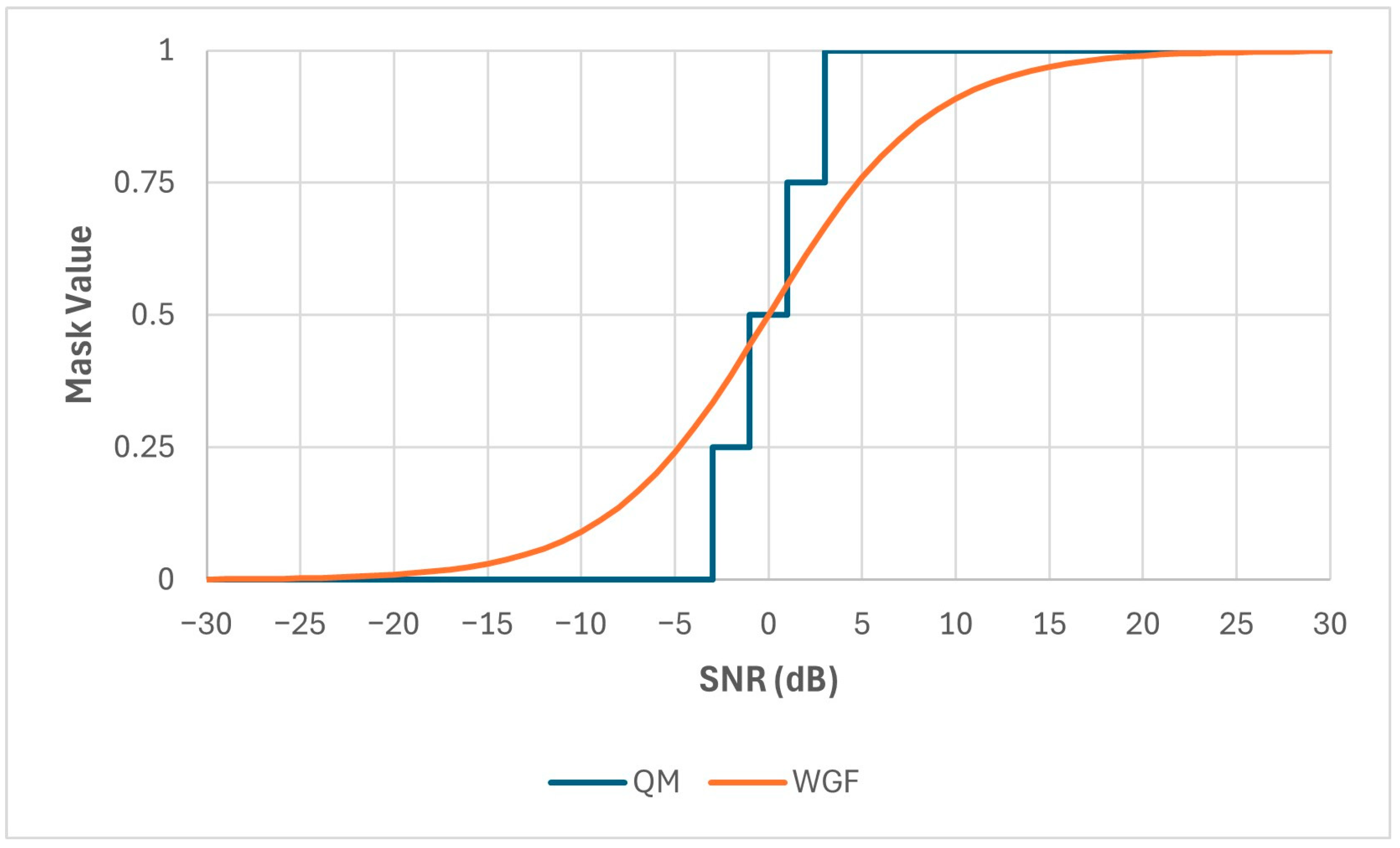
- It proposes the use of a new Quantized Mask (QM), which is an approximation of the Wiener Gain Function (WGF), for the application of speech enhancement in cochlear implants;
- It also proposes another new mask called the PSM+, which is a hybrid of the PSM and the IRM for the same purpose;
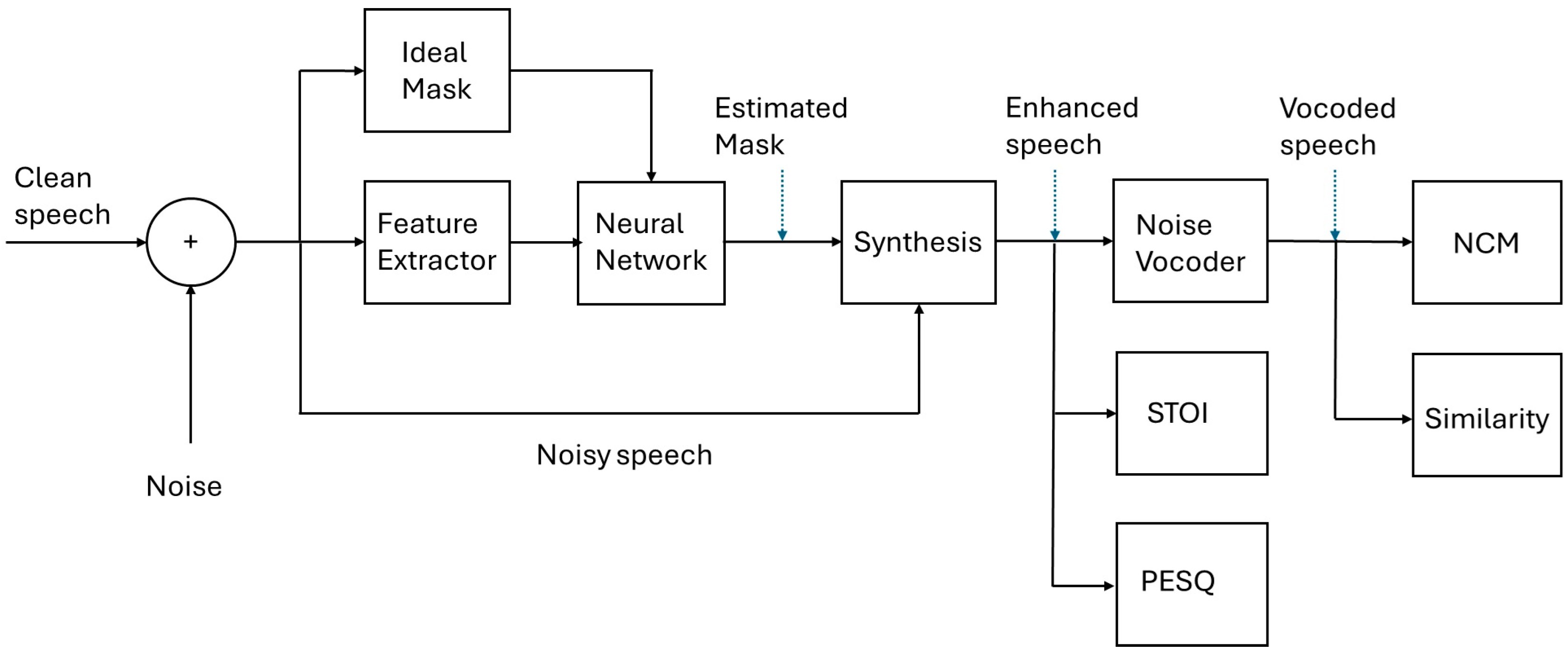
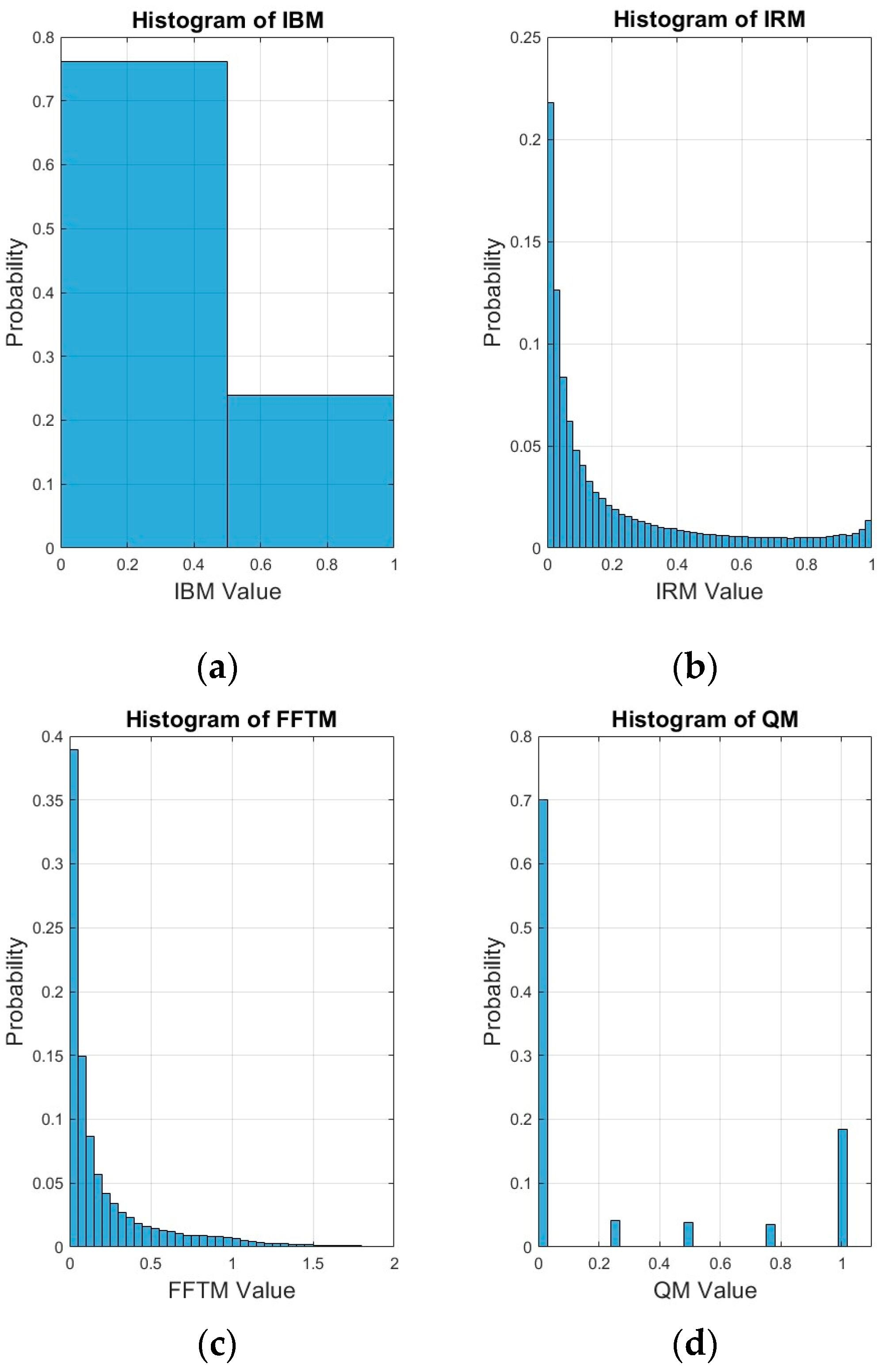
- It compares the performance of these masks to other well-established masks (e.g., IBM, IRM, and FFTM) in terms of speech intelligibility and quality for normal hearing as well as speech intelligibility and similarity for hearing impairment.
2. Background
3. Masks
3.1. Existing Masks
3.2. Proposed Masks
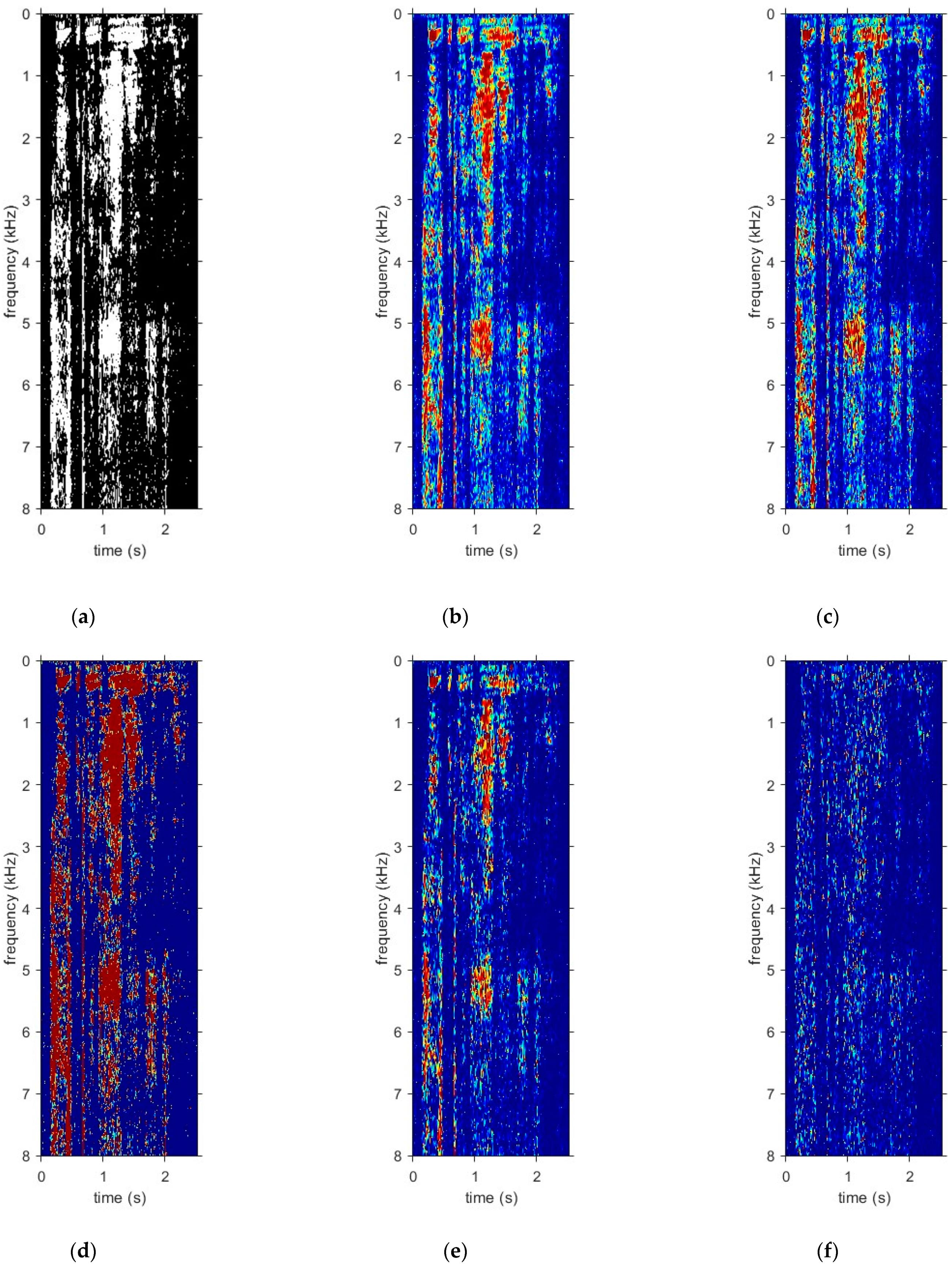
3.3. Examples
4. Materials and Methods
4.1. The Dataset
4.2. Mask Generation
4.3. The Neural Network
4.4. Vocoder Simulation
4.5. Metrics
4.6. Software
5. Results
5.1. Oracle Performance
5.2. Normal Hearing Speech Intelligibility
5.3. Normal Hearing Speech Quality
5.4. Hearing-Impaired Speech Intelligibility
5.5. Hearing-Impaired Speech Similarity
5.5.1. Babble Noise
5.5.2. Speech-Shaped Noise
6. Discussion
7. Conclusions
Author Contributions
Funding
Institutional Review Board Statement
Informed Consent Statement
Data Availability Statement
Conflicts of Interest
References
- Bolner, F.; Goehring, T.; Monaghan, J.; van Dijk, B.; Wouters, J.; Bleeck, S. Speech enhancement based on neural networks applied to cochlear implant coding strategies. In Proceedings of the 2016 IEEE International Conference on Acoustics, Speech and Signal Processing (ICASSP), Shanghai, China, 20–25 March 2016; pp. 6520–6524. [Google Scholar]
- Goehring, T.; Bolner, F.; Monaghan, J.J.; van Dijk, B.; Zarowski, A.; Bleeck, S. Speech enhancement based on neural networks improves speech intelligibility in noise for cochlear implant users. Hear. Res. 2017, 344, 183–194. [Google Scholar] [CrossRef] [PubMed]
- Goehring, T.; Keshavarzi, M.; Carlyon, R.P.; Moore, B.C. Using recurrent neural networks to improve the perception of speech in non-stationary noise by people with cochlear implants. J. Acoust. Soc. Am. 2019, 146, 705–718. [Google Scholar] [CrossRef] [PubMed]
- Chen, J.; Wang, D. Dnn based mask estimation for supervised speech separation. In Audio Source Separation. Signals and Communication Technology; Makino, S., Ed.; Springer: Cham, Switzerland, 2018; pp. 207–235. [Google Scholar]
- Wang, D.; Chen, J. Supervised speech separation based on deep learning: An overview. IEEE/ACM Trans. Audio Speech Lang. Process. 2018, 26, 1702–1726. [Google Scholar] [CrossRef]
- Michelsanti, D.; Tan, Z.-H.; Zhang, S.-X.; Xu, Y.; Yu, M.; Yu, D.; Jensen, J. An overview of deep-learning-based audio-visual speech enhancement and separation. IEEE/ACM Trans. Audio Speech Lang. Process. 2021, 29, 1368–1396. [Google Scholar] [CrossRef]
- Wang, Y.; Wang, D. A deep neural network for time-domain signal reconstruction. In Proceedings of the 2015 IEEE International Conference on Acoustics, Speech and Signal Processing (ICASSP), South Brisbane, QLD, Australia, 19–24 April 2015; pp. 4390–4394. [Google Scholar]
- Nossier, S.A.; Wall, J.; Moniri, M.; Glackin, C.; Cannings, N. Mapping and masking targets comparison using different deep learning based speech enhancement architectures. In Proceedings of the 2020 International Joint Conference on Neural Networks (IJCNN), Glasgow, UK, 19–24 July 2020; pp. 1–8. [Google Scholar]
- Samui, S.; Chakrabarti, I.; Ghosh, S.K. Time–frequency masking based supervised speech enhancement framework using fuzzy deep belief network. Appl. Soft Comput. 2019, 74, 583–602. [Google Scholar] [CrossRef]
- Lee, J.; Skoglund, J.; Shabestary, T.; Kang, H.-G. Phase-sensitive joint learning algorithms for deep learning-based speech enhancement. IEEE Signal Process. Lett. 2018, 25, 1276–1280. [Google Scholar] [CrossRef]
- Heymann, J.; Drude, L.; Haeb-Umbach, R. Neural network based spectral mask estimation for acoustic beamforming. In Proceedings of the 2016 IEEE International Conference on Acoustics, Speech and Signal Processing (ICASSP), Shanghai, China, 20–25 March 2016; pp. 196–200. [Google Scholar]
- Kjems, U.; Boldt, J.B.; Pedersen, M.S.; Lunner, T.; Wang, D. Role of mask pattern in intelligibility of ideal binary-masked noisy speech. J. Acoust. Soc. Am. 2009, 126, 1415–1426. [Google Scholar] [CrossRef]
- Abdullah, S.; Zamani, M.; Demosthenous, A. Towards more efficient DNN-based speech enhancement using quantized correlation mask. IEEE Access 2021, 9, 24350–24362. [Google Scholar] [CrossRef]
- Bao, F.; Abdulla, W.H. Noise masking method based on an effective ratio mask estimation in Gammatone channels. APSIPA Trans. Signal Inf. Process. 2018, 7, e5. [Google Scholar] [CrossRef]
- Bao, F.; Dou, H.-j.; Jia, M.-s.; Bao, C.-c. A novel speech enhancement method using power spectra smooth in wiener filtering. In Proceedings of the Signal and Information Processing Association Annual Summit and Conference (APSIPA), 2014 Asia-Pacific, Siem Reap, Cambodia, 9–12 December 2014; pp. 1–4. [Google Scholar]
- Boldt, J.B.; Ellis, D.P. A simple correlation-based model of intelligibility for nonlinear speech enhancement and separation. In Proceedings of the 2009 17th European Signal Processing Conference, Glasgow, UK, 24–28 August 2009; pp. 1849–1853. [Google Scholar]
- Lang, H.; Yang, J. Learning Ratio Mask with Cascaded Deep Neural Networks for Echo Cancellation in Laser Monitoring Signals. Electronics 2020, 9, 856. [Google Scholar] [CrossRef]
- Choi, H.-S.; Kim, J.-H.; Huh, J.; Kim, A.; Ha, J.-W.; Lee, K. Phase-aware speech enhancement with deep complex u-net. In Proceedings of the International Conference on Learning Representations, Vancouver, BC, Canada, 30 April–3 May 2018. [Google Scholar]
- Erdogan, H.; Hershey, J.R.; Watanabe, S.; Le Roux, J. Phase-sensitive and recognition-boosted speech separation using deep recurrent neural networks. In Proceedings of the 2015 IEEE International Conference on Acoustics, Speech and Signal Processing (ICASSP), South Brisbane, QLD, Australia, 19–24 April 2015; pp. 708–712. [Google Scholar]
- Hasannezhad, M.; Ouyang, Z.; Zhu, W.-P.; Champagne, B. Speech enhancement with phase sensitive mask estimation using a novel hybrid neural network. IEEE Open J. Signal Process. 2021, 2, 136–150. [Google Scholar] [CrossRef]
- Li, H.; Xu, Y.; Ke, D.; Su, K. Improving speech enhancement by focusing on smaller values using relative loss. IET Signal Process. 2020, 14, 374–384. [Google Scholar] [CrossRef]
- Mayer, F.; Williamson, D.S.; Mowlaee, P.; Wang, D. Impact of phase estimation on single-channel speech separation based on time-frequency masking. J. Acoust. Soc. Am. 2017, 141, 4668–4679. [Google Scholar] [CrossRef] [PubMed]
- Ouyang, Z.; Yu, H.; Zhu, W.-P.; Champagne, B. A fully convolutional neural network for complex spectrogram processing in speech enhancement. In Proceedings of the ICASSP 2019–2019 IEEE International Conference on Acoustics, Speech and Signal Processing (ICASSP), Brighton, UK, 12–17 May 2019; pp. 5756–5760. [Google Scholar]
- Tan, K.; Wang, D. Complex spectral mapping with a convolutional recurrent network for monaural speech enhancement. In Proceedings of the ICASSP 2019–2019 IEEE International Conference on Acoustics, Speech and Signal Processing (ICASSP), Brighton, UK, 12–17 May 2019; pp. 6865–6869. [Google Scholar]
- Routray, S.; Mao, Q. Phase sensitive masking-based single channel speech enhancement using conditional generative adversarial network. Comput. Speech Lang. 2022, 71, 101270. [Google Scholar] [CrossRef]
- Wang, X.; Bao, C. Mask estimation incorporating phase-sensitive information for speech enhancement. Appl. Acoust. 2019, 156, 101–112. [Google Scholar] [CrossRef]
- Zhang, Q.; Song, Q.; Ni, Z.; Nicolson, A.; Li, H. Time-frequency attention for monaural speech enhancement. In Proceedings of the ICASSP 2022–2022 IEEE International Conference on Acoustics, Speech and Signal Processing (ICASSP), Singapore, 23–27 May 2022; pp. 7852–7856. [Google Scholar]
- Zheng, N.; Zhang, X.-L. Phase-aware speech enhancement based on deep neural networks. IEEE/ACM Trans. Audio Speech Lang. Process. 2018, 27, 63–76. [Google Scholar] [CrossRef]
- Sivapatham, S.; Kar, A.; Bodile, R.; Mladenovic, V.; Sooraksa, P. A deep neural network-correlation phase sensitive mask based estimation to improve speech intelligibility. Appl. Acoust. 2023, 212, 109592. [Google Scholar] [CrossRef]
- Sowjanya, D.; Sivapatham, S.; Kar, A.; Mladenovic, V. Mask estimation using phase information and inter-channel correlation for speech enhancement. Circuits Syst. Signal Process. 2022, 41, 4117–4135. [Google Scholar] [CrossRef]
- Wang, D. On ideal binary mask as the computational goal of auditory scene analysis. In Speech Separation by Humans and Machines; Springer: Berlin/Heidelberg, Germany, 2005; pp. 181–197. [Google Scholar]
- Wang, Y.; Narayanan, A.; Wang, D. On training targets for supervised speech separation. IEEE/ACM Trans. Audio Speech Lang. Process. 2014, 22, 1849–1858. [Google Scholar] [CrossRef]
- Li, X.; Li, J.; Yan, Y. Ideal Ratio Mask Estimation Using Deep Neural Networks for Monaural Speech Segregation in Noisy Reverberant Conditions. In Proceedings of the Interspeech, Stockholm, Sweden, 20–24 August 2017; pp. 1203–1207. [Google Scholar]
- Wang, Z.; Wang, X.; Li, X.; Fu, Q.; Yan, Y. Oracle performance investigation of the ideal masks. In Proceedings of the 2016 IEEE International Workshop on Acoustic Signal Enhancement (IWAENC), Xi’an, China, 13–16 September 2016; pp. 1–5. [Google Scholar]
- Liang, S.; Liu, W.; Jiang, W.; Xue, W. The optimal ratio time-frequency mask for speech separation in terms of the signal-to-noise ratio. J. Acoust. Soc. Am. 2013, 134, EL452–EL458. [Google Scholar] [CrossRef]
- Xia, S.; Li, H.; Zhang, X. Using optimal ratio mask as training target for supervised speech separation. In Proceedings of the 2017 Asia-Pacific Signal and Information Processing Association Annual Summit and Conference (APSIPA ASC), Kuala Lumpur, Malaysia, 12–15 December 2017; pp. 163–166. [Google Scholar]
- Issa, R.J.; Al-Irhaym, Y.F. Audio source separation using supervised deep neural network. In Proceedings of the Journal of Physics: Conference Series; IOP Publishing: Bristol, UK, 2021; p. 022077. [Google Scholar]
- Williamson, D.S.; Wang, Y.; Wang, D. Complex ratio masking for monaural speech separation. IEEE/ACM Trans. Audio Speech Lang. Process. 2015, 24, 483–492. [Google Scholar] [CrossRef] [PubMed]
- Williamson, D.S.; Wang, D. Time-frequency masking in the complex domain for speech dereverberation and denoising. IEEE/ACM Trans. Audio Speech Lang. Process. 2017, 25, 1492–1501. [Google Scholar] [CrossRef] [PubMed]
- Hu, Y.; Loizou, P.C. A new sound coding strategy for suppressing noise in cochlear implants. J. Acoust. Soc. Am. 2008, 124, 498–509. [Google Scholar] [CrossRef] [PubMed]
- Hasan, T.; Hansen, J.H. Acoustic factor analysis for robust speaker verification. IEEE Trans. Audio Speech Lang. Process. 2012, 21, 842–853. [Google Scholar] [CrossRef]
- Zhou, L.; Jiang, W.; Xu, J.; Wen, F.; Liu, P. Masks fusion with multi-target learning for speech enhancement. arXiv 2021, arXiv:2109.11164. [Google Scholar]
- Rothauser, E. IEEE recommended practice for speech quality measurements. IEEE Trans. Audio Electroacoust. 1969, 17, 225–246. [Google Scholar]
- Loizou, P.C. Speech Enhancement: Theory and Practice; CRC Press: Boca Raton, FL, USA, 2013. [Google Scholar]
- Liu, Y.; Zhang, H.; Zhang, X. Using Shifted Real Spectrum Mask as Training Target for Supervised Speech Separation. In Proceedings of the Interspeech, Hyderabad, India, 2–6 September 2018; pp. 1151–1155. [Google Scholar]
- Henry, F.; Parsi, A.; Glavin, M.; Jones, E. Experimental Investigation of Acoustic Features to Optimize Intelligibility in Cochlear Implants. Sensors 2023, 23, 7553. [Google Scholar] [CrossRef] [PubMed]
- Healy, E.W.; Yoho, S.E.; Wang, Y.; Wang, D. An algorithm to improve speech recognition in noise for hearing-impaired listeners. J. Acoust. Soc. Am. 2013, 134, 3029–3038. [Google Scholar] [CrossRef]
- Cychosz, M.; Winn, M.B.; Goupell, M.J. How to vocode: Using channel vocoders for cochlear-implant research. J. Acoust. Soc. Am. 2024, 155, 2407–2437. [Google Scholar] [CrossRef]
- Falk, T.H.; Parsa, V.; Santos, J.F.; Arehart, K.; Hazrati, O.; Huber, R.; Kates, J.M.; Scollie, S. Objective quality and intelligibility prediction for users of assistive listening devices: Advantages and limitations of existing tools. IEEE Signal Process. Mag. 2015, 32, 114–124. [Google Scholar] [CrossRef]
- Cosentino, S.; Marquardt, T.; McAlpine, D.; Falk, T.H. Towards objective measures of speech intelligibility for cochlear implant users in reverberant environments. In Proceedings of the 2012 11th International Conference on Information Science, Signal Processing and their Applications (ISSPA), Montreal, QC, Canada, 2–5 July 2012; pp. 666–671. [Google Scholar]
- Santos, J.F.; Cosentino, S.; Hazrati, O.; Loizou, P.C.; Falk, T.H. Performance comparison of intrusive objective speech intelligibility and quality metrics for cochlear implant users. In Proceedings of the Thirteenth Annual Conference of the International Speech Communication Association, Portland, OR, USA, 9–13 September 2012. [Google Scholar]
- Kokkinakis, K.; Loizou, P.C. Evaluation of objective measures for quality assessment of reverberant speech. In Proceedings of the 2011 IEEE International Conference on Acoustics, Speech and Signal Processing (ICASSP), Prague, Czech Republic, 22–27 May 2011; pp. 2420–2423. [Google Scholar]
- Hu, Y.; Loizou, P.C. Evaluation of objective quality measures for speech enhancement. IEEE Trans. Audio Speech Lang. Process. 2007, 16, 229–238. [Google Scholar] [CrossRef]
- Taal, C.H.; Hendriks, R.C.; Heusdens, R.; Jensen, J. An algorithm for intelligibility prediction of time–frequency weighted noisy speech. IEEE Trans. Audio Speech Lang. Process. 2011, 19, 2125–2136. [Google Scholar] [CrossRef]
- Taal, C.H.; Hendriks, R.C.; Heusdens, R.; Jensen, J. A short-time objective intelligibility measure for time-frequency weighted noisy speech. In Proceedings of the 2010 IEEE International Conference on Acoustics, Speech and Signal Processing, Dallas, TX, USA, 14–19 March 2010; pp. 4214–4217. [Google Scholar]
- Rix, A.W.; Beerends, J.G.; Hollier, M.P.; Hekstra, A.P. Perceptual evaluation of speech quality (PESQ)-a new method for speech quality assessment of telephone networks and codecs. In Proceedings of the 2001 IEEE International Conference on Acoustics, Speech, and Signal Processing. Proceedings (Cat. No. 01CH37221), Salt Lake City, UT, USA, 7–11 May 2001; pp. 749–752. [Google Scholar]
- Kurittu, A.; Samela, J.; Lakaniemi, A.; Mattila, V.-v.; Zacharov, N. Application and Verfication of the Objective Quality Assessment Method According to ITU Recommendation Series ITU-T P. 862. J. Audio Eng. Soc. 2006, 54, 1189–1202. [Google Scholar]
- Holube, I.; Kollmeier, B. Speech intelligibility prediction in hearing-impaired listeners based on a psychoacoustically motivated perception model. J. Acoust. Soc. Am. 1996, 100, 1703–1716. [Google Scholar] [CrossRef]
- Lai, Y.-H.; Chen, F.; Wang, S.-S.; Lu, X.; Tsao, Y.; Lee, C.-H. A deep denoising autoencoder approach to improving the intelligibility of vocoded speech in cochlear implant simulation. IEEE Trans. Biomed. Eng. 2017, 64, 1568–1578. [Google Scholar] [CrossRef] [PubMed]
- Kalaivani, S.; Thakur, R.S. Modified Hidden Markov Model for Speaker Identification System. Int. J. Adv. Comput. Electron. Eng. 2017, 2, 1–7. [Google Scholar]
- Thakur, A.S.; Sahayam, N. Speech recognition using euclidean distance. Int. J. Emerg. Technol. Adv. Eng. 2013, 3, 587–590. [Google Scholar]
- Park, M.W.; Lee, E.C. Similarity measurement method between two songs by using the conditional Euclidean distance. Wseas Trans. Inf. Sci. Appl. 2013, 10, 12. [Google Scholar]
- Cha, S.-H. Comprehensive survey on distance/similarity measures between probability density functions. Int. J. Math. Models Methods Appl. Sci. 2007, 1, 300–307. [Google Scholar]
- Newman, R.; Chatterjee, M. Toddlers’ recognition of noise-vocoded speech. J. Acoust. Soc. Am. 2013, 133, 483–494. [Google Scholar] [CrossRef]
- Hu, Y.; Liu, Y.; Lv, S.; Xing, M.; Zhang, S.; Fu, Y.; Wu, J.; Zhang, B.; Xie, L. DCCRN: Deep complex convolution recurrent network for phase-aware speech enhancement. arXiv 2020, arXiv:2008.00264. [Google Scholar]


| Mask | Mix (babble) | IBM | IRM | FFTM | QM | PSM |
| mean | 0.5483 | 0.8761 | 0.9171 | 0.9364 | 0.8861 | 0.9343 |
| median | 0.5502 | 0.8787 | 0.9188 | 0.9379 | 0.8883 | 0.9356 |
| standard deviation | 0.055 | 0.0213 | 0.0156 | 0.0136 | 0.0199 | 0.0134 |
| Mask | Mix (SSN) | IBM | IRM | FFTM | QM | PSM |
| mean | 0.574 | 0.872 | 0.9114 | 0.9321 | 0.8825 | 0.9288 |
| median | 0.5789 | 0.8746 | 0.9128 | 0.9338 | 0.8846 | 0.9302 |
| standard deviation | 0.0524 | 0.0211 | 0.0157 | 0.0143 | 0.0196 | 0.0143 |
| Mask | Mix (factory) | IBM | IRM | FFTM | QM | PSM |
| mean | 0.5525 | 0.8717 | 0.9172 | 0.937 | 0.8821 | 0.935 |
| median | 0.5559 | 0.8737 | 0.9187 | 0.9385 | 0.8853 | 0.9367 |
| standard deviation | 0.0492 | 0.023 | 0.0149 | 0.013 | 0.0212 | 0.0129 |
| Noise | SNR (dB) | Mask | |||||
|---|---|---|---|---|---|---|---|
| Mix | IBM | IRM | FFTM | QM | PSM+ | ||
| babble | −5 | 0.5599 | 0.6328 | 0.6333 | 0.6396 | 0.6326 | 0.6358 |
| babble | 0 | 0.6738 | 0.7717 | 0.7659 | 0.775 | 0.7693 | 0.7737 |
| babble | 5 | 0.7889 | 0.8684 | 0.8639 | 0.8677 | 0.8686 | 0.8701 |
| SSN | −5 | 0.5849 | 0.7231 | 0.7256 | 0.7305 | 0.7231 | 0.7307 |
| SSN | 0 | 0.7047 | 0.8322 | 0.8289 | 0.8363 | 0.8328 | 0.838 |
| SSN | 5 | 0.8216 | 0.9043 | 0.9017 | 0.9072 | 0.9046 | 0.9092 |
| MEAN | 0.688967 | 0.78875 | 0.78655 | 0.792717 | 0.7885 | 0.792917 | |
| Noise | SNR (dB) | Mask | |||||
|---|---|---|---|---|---|---|---|
| Mix | IBM | IRM | FFTM | QM | PSM+ | ||
| babble | −5 | 1.0692 | 1.1004 | 1.1195 | 1.1142 | 1.1038 | 1.1348 |
| babble | 0 | 1.0895 | 1.2511 | 1.2541 | 1.2376 | 1.2622 | 1.2932 |
| babble | 5 | 1.1978 | 1.6059 | 1.5391 | 1.5191 | 1.6156 | 1.5774 |
| SSN | −5 | 1.0479 | 1.1595 | 1.1675 | 1.1723 | 1.1618 | 1.1904 |
| SSN | 0 | 1.0787 | 1.3317 | 1.3161 | 1.3365 | 1.3356 | 1.3676 |
| SSN | 5 | 1.1597 | 1.6618 | 1.605 | 1.6123 | 1.6704 | 1.7079 |
| MEAN | 1.107133 | 1.351733 | 1.33355 | 1.332 | 1.358233 | 1.37855 | |
| Noise | SNR (dB) | Mask | |||||
|---|---|---|---|---|---|---|---|
| Mix | IBM | IRM | FFTM | QM | PSM+ | ||
| babble | −5 | 0.3651 | 0.5385 | 0.5492 | 0.5482 | 0.5448 | 0.555 |
| babble | 0 | 0.5626 | 0.7121 | 0.7137 | 0.7109 | 0.7166 | 0.7157 |
| babble | 5 | 0.7149 | 0.813 | 0.8091 | 0.8063 | 0.8131 | 0.8103 |
| SSN | −5 | 0.4456 | 0.701 | 0.7101 | 0.7075 | 0.7036 | 0.7126 |
| SSN | 0 | 0.631 | 0.8018 | 0.7984 | 0.7953 | 0.802 | 0.8001 |
| SSN | 5 | 0.756 | 0.8469 | 0.8469 | 0.8447 | 0.8469 | 0.8468 |
| MEAN | 0.5792 | 0.73555 | 0.7379 | 0.73548 | 0.737833 | 0.740083 | |
| Metric/Mask | Mix | IBM | IRM | FFTM | QM | PSM+ |
|---|---|---|---|---|---|---|
| Lp | 0.7765 | 0.8632 | 0.8673 | 0.8585 | 0.8714 | 0.8716 |
| L1 | 0.6722 | 0.8401 | 0.8417 | 0.8305 | 0.8485 | 0.8412 |
| Intersection | 0.3339 | 0.5356 | 0.5389 | 0.5243 | 0.5472 | 0.5409 |
| Inner Product | 0.1999 | 0.4138 | 0.4228 | 0.4082 | 0.428 | 0.431 |
| Fidelity | 0.7441 | 0.9164 | 0.9189 | 0.9115 | 0.9228 | 0.9196 |
| Squared L2 | 0.9376 | 0.9754 | 0.9763 | 0.9735 | 0.9778 | 0.9773 |
| Shannon’s Entropy | 0.5999 | 0.1164 | 0.1102 | 0.1267 | 0.102 | 0.1074 |
| Combinations | 0.6368 | 0.8544 | 0.8586 | 0.8463 | 0.8649 | 0.8612 |
| Correlation | 0.5724 | 0.8756 | 0.8754 | 0.8572 | 0.8875 | 0.8789 |
| Metric/Mask | Mix | IBM | IRM | FFTM | QM | PSM+ |
|---|---|---|---|---|---|---|
| Lp | 0.7891 | 0.9136 | 0.9023 | 0.8889 | 0.9356 | 0.9062 |
| L1 | 0.717 | 0.8936 | 0.88 | 0.8661 | 0.911 | 0.8793 |
| Intersection | 0.3834 | 0.6097 | 0.5916 | 0.5719 | 0.6364 | 0.593 |
| Inner Product | 0.2452 | 0.4869 | 0.4744 | 0.4563 | 0.5125 | 0.4808 |
| Fidelity | 0.8017 | 0.9505 | 0.9431 | 0.9353 | 0.9599 | 0.9434 |
| Squared L2 | 0.945 | 0.9889 | 0.986 | 0.9827 | 0.9934 | 0.9869 |
| Shannon’s Entropy | 0.4296 | 0.0479 | 0.0602 | 0.0753 | 0.0322 | 0.0591 |
| Combinations | 0.6991 | 0.9137 | 0.9008 | 0.886 | 0.9332 | 0.9026 |
| Correlation | 0.6418 | 0.9497 | 0.9317 | 0.9134 | 0.972 | 0.9353 |
| Metric/Mask | Mix | IBM | IRM | FFTM | QM | PSM+ |
|---|---|---|---|---|---|---|
| Lp | 0.8103 | 0.9675 | 0.929 | 0.9281 | 0.9672 | 0.9458 |
| L1 | 0.7685 | 0.9406 | 0.9088 | 0.9079 | 0.9402 | 0.9208 |
| Intersection | 0.4434 | 0.6793 | 0.6311 | 0.6297 | 0.6788 | 0.6505 |
| Inner Product | 0.3084 | 0.5416 | 0.5045 | 0.5035 | 0.5414 | 0.5223 |
| Fidelity | 0.856 | 0.9728 | 0.9581 | 0.958 | 0.9726 | 0.9641 |
| Squared L2 | 0.9555 | 0.9982 | 0.9921 | 0.992 | 0.9982 | 0.9951 |
| Shannon’s Entropy | 0.2717 | 0.0152 | 0.0354 | 0.0357 | 0.0154 | 0.0263 |
| Combinations | 0.7662 | 0.9609 | 0.9292 | 0.9283 | 0.9607 | 0.9427 |
| Correlation | 0.7275 | 0.9954 | 0.9643 | 0.9642 | 0.9953 | 0.9794 |
| Metric/Mask | Mix | IBM | IRM | FFTM | QM | PSM+ |
|---|---|---|---|---|---|---|
| Lp | 0.767 | 0.8853 | 0.8814 | 0.8796 | 0.8945 | 0.8949 |
| L1 | 0.6368 | 0.866 | 0.8564 | 0.854 | 0.8744 | 0.8579 |
| Intersection | 0.2954 | 0.5699 | 0.5592 | 0.5562 | 0.5823 | 0.5682 |
| Inner Product | 0.1651 | 0.4504 | 0.447 | 0.4444 | 0.4633 | 0.4694 |
| Fidelity | 0.6921 | 0.9339 | 0.9291 | 0.9275 | 0.9391 | 0.9321 |
| Squared L2 | 0.9317 | 0.982 | 0.9804 | 0.9798 | 0.9843 | 0.9836 |
| Shannon’s Entropy | 0.757 | 0.0785 | 0.0866 | 0.0897 | 0.068 | 0.0779 |
| Combinations | 0.5831 | 0.8838 | 0.8766 | 0.8742 | 0.8936 | 0.8855 |
| Correlation | 0.5076 | 0.9117 | 0.8969 | 0.8925 | 0.9238 | 0.9134 |
| Metric/Mask | Mix | IBM | IRM | FFTM | QM | PSM+ |
|---|---|---|---|---|---|---|
| Lp | 0.7813 | 0.9645 | 0.9231 | 0.9272 | 0.9641 | 0.9408 |
| L1 | 0.6939 | 0.9378 | 0.9022 | 0.9063 | 0.9376 | 0.9101 |
| Intersection | 0.3573 | 0.6755 | 0.622 | 0.6278 | 0.6751 | 0.6386 |
| Inner Product | 0.22 | 0.5379 | 0.4984 | 0.5024 | 0.5372 | 0.52 |
| Fidelity | 0.7738 | 0.9712 | 0.9545 | 0.9567 | 0.971 | 0.9592 |
| Squared L2 | 0.9404 | 0.9978 | 0.9907 | 0.9915 | 0.9977 | 0.994 |
| Shannon’s Entropy | 0.5127 | 0.0169 | 0.0409 | 0.0376 | 0.0171 | 0.033 |
| Combinations | 0.6674 | 0.9583 | 0.9229 | 0.9269 | 0.9581 | 0.9352 |
| Correlation | 0.5972 | 0.9935 | 0.9572 | 0.9615 | 0.9931 | 0.9733 |
| Metric/Mask | Mix | IBM | IRM | FFTM | QM | PSM+ |
|---|---|---|---|---|---|---|
| Lp | 0.8012 | 0.9556 | 0.9512 | 0.9473 | 0.9518 | 0.9637 |
| L1 | 0.7501 | 0.9312 | 0.9306 | 0.9279 | 0.9276 | 0.9376 |
| Intersection | 0.4216 | 0.6659 | 0.6621 | 0.6578 | 0.661 | 0.6751 |
| Inner Product | 0.2847 | 0.5451 | 0.5245 | 0.5208 | 0.5447 | 0.5369 |
| Fidelity | 0.8373 | 0.9704 | 0.9675 | 0.9664 | 0.9693 | 0.9708 |
| Squared L2 | 0.951 | 0.997 | 0.9959 | 0.9953 | 0.9966 | 0.9976 |
| Shannon’s Entropy | 0.3248 | 0.0179 | 0.0221 | 0.0236 | 0.0191 | 0.0179 |
| Combinations | 0.7427 | 0.9523 | 0.9496 | 0.9466 | 0.9492 | 0.958 |
| Correlation | 0.6897 | 0.9947 | 0.9835 | 0.981 | 0.9941 | 0.9915 |
| Mask | Noise | SNR | Wang et al. | This Study |
| Mix | babble | −5 | 0.55 | 0.5599 |
| IBM | babble | −5 | 0.63 | 0.6328 |
| IRM | babble | −5 | 0.63 | 0.6333 |
| FFTM | babble | −5 | 0.65 | 0.6396 |
| Mix | SSN | −5 | 0.57 | 0.5849 |
| IBM | SSN | −5 | 0.72 | 0.7231 |
| IRM | SSN | −5 | 0.73 | 0.7256 |
| FFTM | SSN | −5 | 0.74 | 0.7305 |
| Mix | babble | 0 | 0.66 | 0.6738 |
| IBM | babble | 0 | 0.76 | 0.7717 |
| IRM | babble | 0 | 0.76 | 0.7659 |
| FFTM | babble | 0 | 0.77 | 0.775 |
| Mix | SSN | 0 | 0.69 | 0.7047 |
| IBM | SSN | 0 | 0.82 | 0.8322 |
| IRM | SSN | 0 | 0.83 | 0.8289 |
| FFTM | SSN | 0 | 0.83 | 0.8363 |
| Mix | babble | 5 | 0.77 | 0.7889 |
| IBM | babble | 5 | 0.86 | 0.8684 |
| IRM | babble | 5 | 0.86 | 0.8639 |
| FFTM | babble | 5 | 0.85 | 0.8677 |
| Mix | SSN | 5 | 0.81 | 0.8216 |
| IBM | SSN | 5 | 0.87 | 0.9043 |
| IRM | SSN | 5 | 0.88 | 0.9017 |
| FFTM | SSN | 5 | 0.85 | 0.9072 |
Disclaimer/Publisher’s Note: The statements, opinions and data contained in all publications are solely those of the individual author(s) and contributor(s) and not of MDPI and/or the editor(s). MDPI and/or the editor(s) disclaim responsibility for any injury to people or property resulting from any ideas, methods, instructions or products referred to in the content. |
© 2024 by the authors. Licensee MDPI, Basel, Switzerland. This article is an open access article distributed under the terms and conditions of the Creative Commons Attribution (CC BY) license (https://creativecommons.org/licenses/by/4.0/).
Share and Cite
Henry, F.; Glavin, M.; Jones, E.; Parsi, A. Impact of Mask Type as Training Target for Speech Intelligibility and Quality in Cochlear-Implant Noise Reduction. Sensors 2024, 24, 6614. https://doi.org/10.3390/s24206614
Henry F, Glavin M, Jones E, Parsi A. Impact of Mask Type as Training Target for Speech Intelligibility and Quality in Cochlear-Implant Noise Reduction. Sensors. 2024; 24(20):6614. https://doi.org/10.3390/s24206614
Chicago/Turabian StyleHenry, Fergal, Martin Glavin, Edward Jones, and Ashkan Parsi. 2024. "Impact of Mask Type as Training Target for Speech Intelligibility and Quality in Cochlear-Implant Noise Reduction" Sensors 24, no. 20: 6614. https://doi.org/10.3390/s24206614
APA StyleHenry, F., Glavin, M., Jones, E., & Parsi, A. (2024). Impact of Mask Type as Training Target for Speech Intelligibility and Quality in Cochlear-Implant Noise Reduction. Sensors, 24(20), 6614. https://doi.org/10.3390/s24206614