Performance Analysis of Centralized Cooperative Schemes for Compressed Sensing

Abstract

This paper presents a performance analysis of centralized spectrum sensing based on compressed measurements. We assume cooperative sensing, where unlicensed users individually perform compressed sensing and send their results to a fusion center, which makes the final decision about the presence or absence of a licensed user signal. Several cooperation schemes are considered, such as and-rule, or-rule, majority voting, soft equal-gain combining (EGC). The proposed analysis provides simplified closed-form expressions that calculate the required number of sensors, the required number of samples, the required compression ratio, and the required signal-to-noise ratio (SNR) as a function of the probability of detection and the probability of the false alarm of the fusion center and of the sensors. The resulting expressions are derived by exploiting some accurate approximations of the test statistics of the fusion center and of the sensors, equipped with energy detectors. The obtained results are useful, especially for a low number of sensors and low sample sizes, where conventional closed-form expressions based on the central limit theorem (CLT) fail to provide accurate approximations. The proposed analysis also allows the self-computation of the performance of each sensor and of the fusion center with reduced complexity.

1. Introduction

Cooperative spectrum sensing (CSS) [1,2,3] is a key component of a cognitive radio (CR) network and aims to discover whether some resources are available for signal transmission or not in a given area. Using CSS, unlicensed secondary users (SUs) collaboratively detect the presence or absence of a signal transmitted by a licensed primary user (PU) to understand whether a given channel is already occupied by a PU or free and hence available for SU signal transmission.

One crucial factor of CSS is the amount of data used for sensing purposes. In general, both false alarm (FA) and detection performances improve by increasing the number of SUs and the time spent for sensing at the expense of increased computational processing. Hence, two fundamental parameters are the number of SU sensors and the number of samples used by an SU. Compressed sensing [4,5] is often employed to reduce the number of samples to the reduce complexity. The need for power consumption reduction also requires sensors that are in sleeping mode (i.e., inactive) for a certain fraction of time, to save energy.

A second major factor of CSS is the sensing algorithm of the SUs. The choice of this algorithm mostly depends on the available information about the structure of the PU signal [6,7,8,9,10,11,12,13]. Matched filtering and feature extraction presuppose that the SUs have some knowledge about the PU signal properties. On the other hand, an energy detector (ED) simply monitors the received energy in a specific time–frequency resource, and therefore is more versatile and suitable for those users without knowledge of the PU signal properties. The popularity of the ED is widespread [13,14,15,16,17,18,19,20,21,22,23,24,25,26,27], so that the ED is often also used as a baseline for comparison purposes. Consequently, this paper focuses on SU sensors equipped with EDs.

The third important factor of CSS is the type of cooperation. Indeed, the sensing results acquired by the SUs may be combined either by a centralized fusion center (FC) or using a distributed approach. Herein, we focus on a centralized approach wherein an FC collects the reports of the SUs. In addition, the fusion operation can be performed in several different ways [28,29,30,31,32,33,34,35,36,37,38,39,40,41,42,43,44,45,46,47,48,49,50,51,52]: this paper mainly focuses on hard reporting (HR), where the SUs report their hard decisions to the FC. Anyway, we also consider a soft reporting (SR) case, where the SUs report their soft decisions to the FC, which aggregates these values using equal-gain combining (EGC).

Although there exist several performance analyses of CSS with EDs [15,16,18,19,23,24,25,26,27], most of the existing approaches either involve complicated multidimensional functions or have low accuracy. For instance, the exact calculation of the receiver operating characteristic (ROC) of the ED requires the inversion of a chi-squared distribution function [16,19,23,24,25], but this computation can be energy-demanding for low-cost sensors. On the other hand, a popular alternative approach is the Gaussian approximation (GA) for the test statistic of the ED [15,18,26,27]; however, the accuracy of the obtained ROC is reduced, especially when the number of samples is low. Similarly, when the FC applies a majority-voting (MV) rule, an exact analysis of the required number of SUs involves complicated functions like the incomplete beta function [53] and its inverse, whereas GA approaches based on the central limit theorem (CLT) may be inaccurate, especially when the number of sensors is low.

This paper aims at closing the gap between the accurate-but-complicated performance analyses and simple-but-inaccurate performance analyses of CSS with EDs. Specifically, this paper proposes simple low-complexity accurate approximations in such a way that the performance assessment can be also self-performed by low-cost sensors and by a low-energy FC. The proposed approximations are obtained by modifying and adapting the methods of probability distribution approximation derived several decades ago [54,55,56,57,58,59,60,61,62,63]. The main contributions of this paper can be summarized as follows.

• For the HR case, we propose closed-form expressions for the number of active sensors required by an FC to achieve a target performance, assuming SUs with a given performance. Several fusion rules are considered: and-rule, or-rule, and MV-rule. In contrast to existing work, the proposed expressions have both accuracy and low complexity.
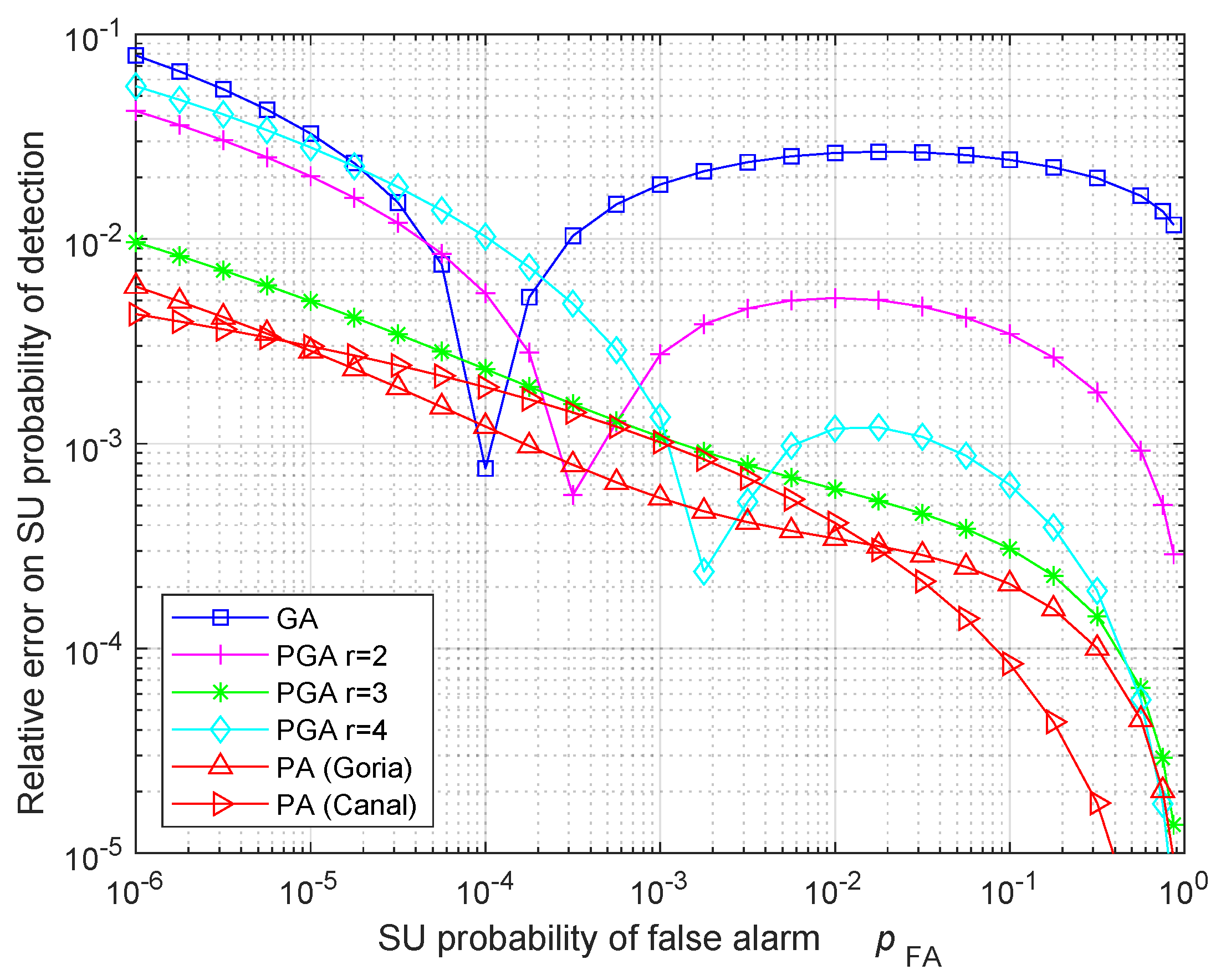
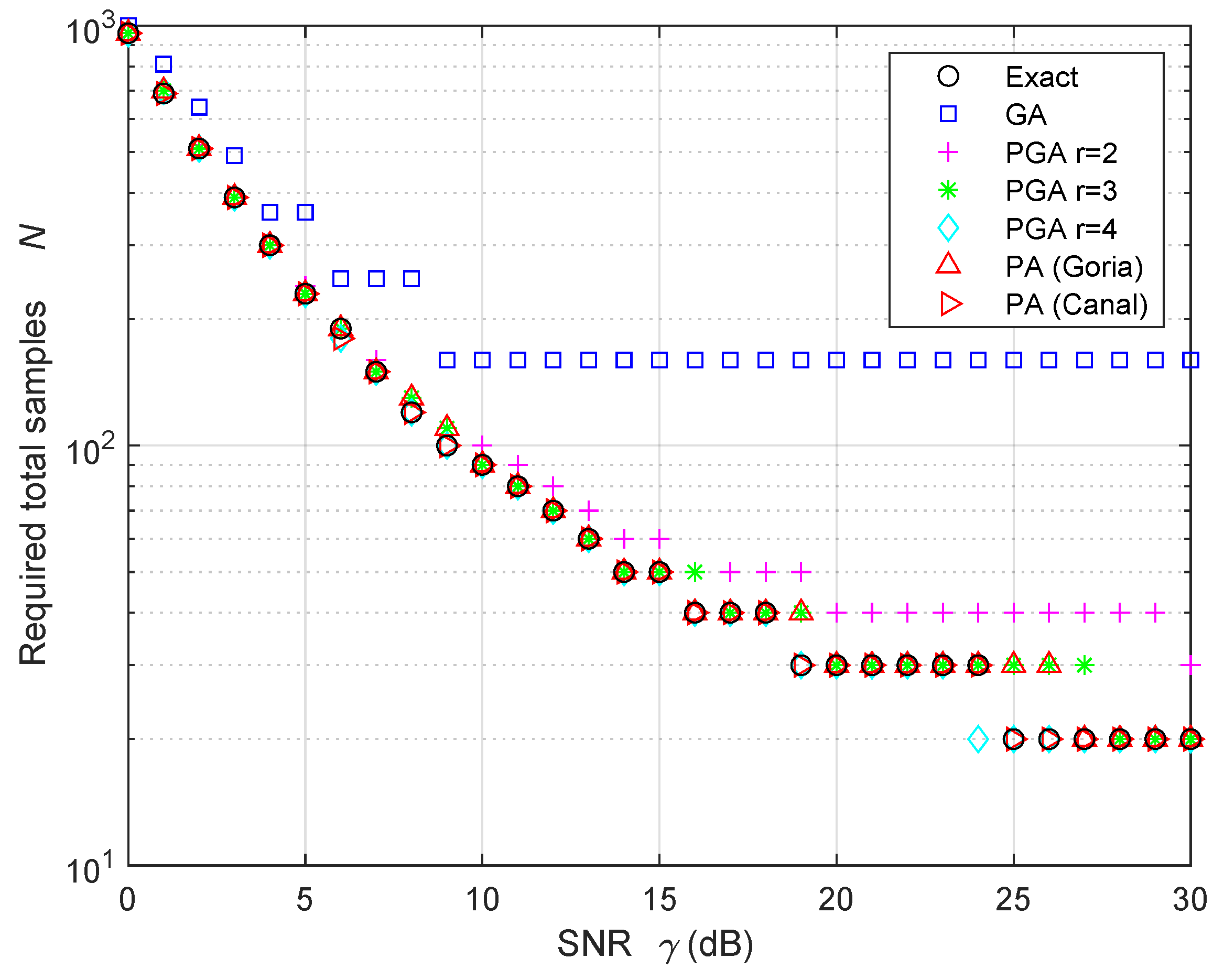
• For the HR case, we propose closed-form expressions for the number of compressed samples required by an ED to achieve a target performance, assuming a given PU signal-to-noise ratio (SNR). Again, the proposed expressions have both accuracy and low complexity, thereby enabling low-energy self-computation at the SU side. Previous work in [64,65,66] only includes a limited subset of expressions, mainly for conventional non-cooperative sensing, whereas this paper derives a complete performance analysis valid for cooperative compressed sensing.
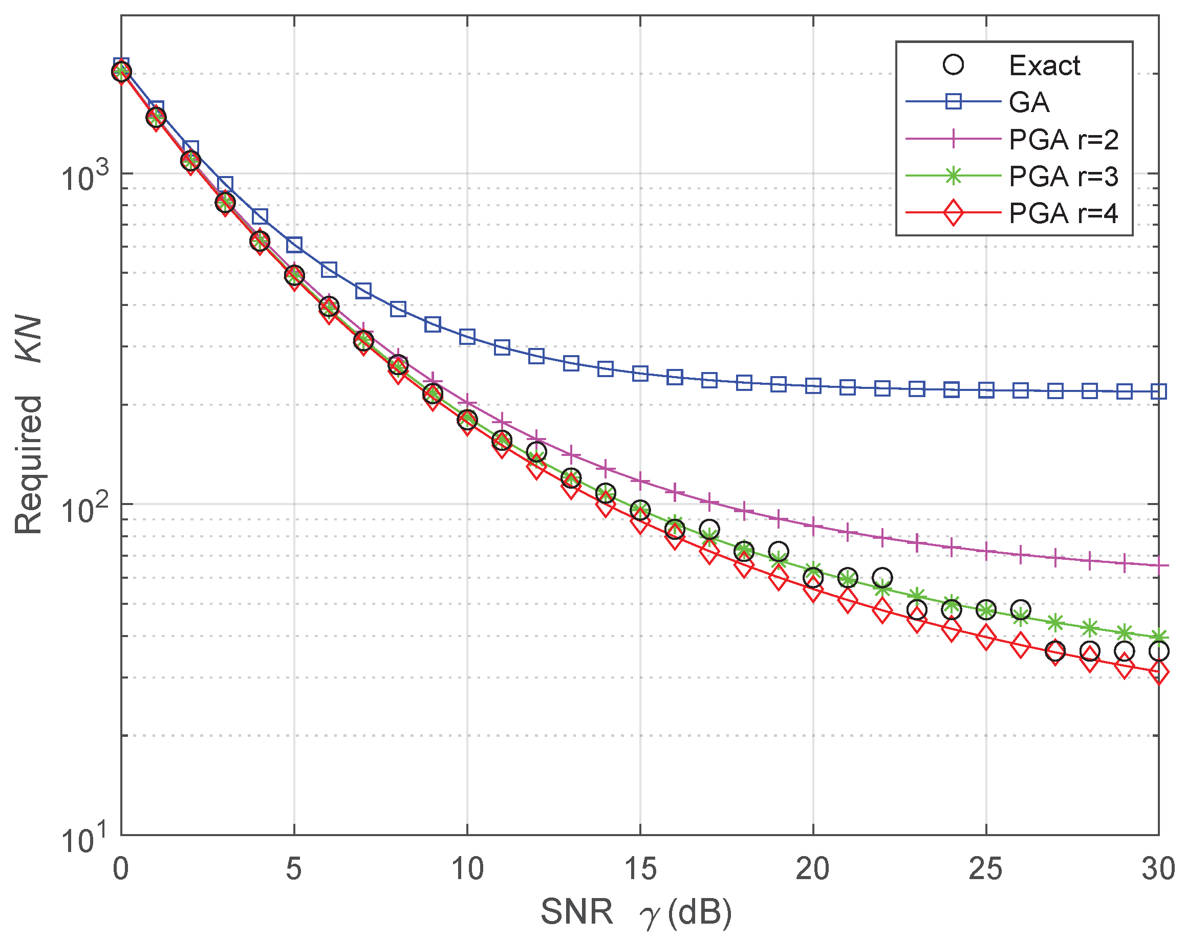
• For the SR case, we propose closed-form expressions for the aggregate number of samples required by an FC to achieve a target performance. Also, in this case, the proposed expressions combine accuracy with low complexity.

The remainder of this paper is structured as follows. Section 2 outlines the state of the art, while Section 3 introduces the system model. Section 4 develops the approximated performance analysis. Numerical results are presented in Section 5 to validate the proposed approximations, and some concluding remarks are drawn in Section 6.

2. State of the Art

In this section, we focus on the literature about CSS performance analysis in terms of the required number of users and required number of samples. For what concerns the number of sensors to warranty (at the FC) a predefined probability of detection and a predefined probability of FA, let us assume HR with MV-rule and sensors with the same statistics. In this case, the probabilities of detection and of FA are expressed as a sum [6,15] whose result is expressed by the incomplete beta function [53]. The most common approach for inverting this function is to apply general-purpose software routines, such as in [29,30,33,34,41,45,67,68,69], without an explicit closed-form solution and without complexity analysis. Therefore, the complexity of the FC performance self-estimation may potentially be large, especially when accurate self-estimation is required. A low-complexity approximation applies the CLT, but several other approaches are possible, with greater accuracy and tolerable complexity. For the MV-rule, Section 4.1 of this paper will present six low-complexity approximations, whose accuracy will be compared in Section 5.

For what concerns the number of samples required to obtain (at the SU) the desired probabilities of detection and FA, a summary of relevant results is given in [15], which considers two models for the PU signal received by the SUs, namely the deterministic and random models. In the literature, the deterministic model is more popular [17,20,21], and sometimes includes random fading [19,23,25,26] and diversity [9,24]. On the other side, the random model for the PU signal [6] is less common. However, the deterministic model is only appropriate when the SUs are perfectly synchronous and do not apply compressed sensing. When the SU sensors are partially asynchronous or apply compressed sensing, the EDs of the different SUs collect samples that are different in time; therefore, a random PU signal model seems more reasonable. In any case, the results in [15] show that the exact value for the required sample size is significantly different from the CLT-approximated sample size obtained using a Gaussian approach for both deterministic and random models. For the deterministic model, some improved approximations are proposed in [17,20,21], but for the random model, there exist less results [64,65,66]. Section 4.2 of this paper will present three low-complexity approaches, whose accuracy will be compared in Section 5.

3. System Model

First, in Section 3.1, we briefly describe the CSS system model without using mathematical equations, in order to give a quick general overview. Second, in Section 3.2, we present a detailed statistical signal model based on mathematical equations, which are instrumental for the performance derivation of the considered CSS scheme in Section 4.

3.1. Overview of Centralized Cooperative Sensing

We consider a CR network with multiple sensors acting as SUs and a centralized FC. We assume that the SUs and the FC are located in a specific area. The aim is to sense the presence or absence of a PU signal in a given frequency band. It is assumed that the PU is located outside the area where the SUs and the FC are located. The centralized CSS is performed in three phases. In the first phase, the SUs perform compressed spectrum sensing using an ED. The sensing results of the SUs may be either binary hard decisions or soft decisions. In the second phase, the SUs, or a fraction of them, report their sensing results to the FC, which collects the received results. In the case of sensing results with binary hard decisions, we refer to this second phase as HR. In the case of sensing results with soft decisions, we refer to this second phase as SR. In the third phase, the FC makes a final decision based on the reports received from the SUs. In the case of HR, the FC collects the received binary decisions of the SUs and performs a final decision using a given rule, such as the and-rule, the or-rule, or the MV-rule. In the case of SR, the FC collects the received nonbinary results and performs a soft EGC to obtain the test statistics for the final decision.

3.2. Statistical Signal Model

We consider a CR network with K SUs equipped with EDs. As in [14], we assume that the PU transmitter is located far away from the area where the K SUs are located. We assume that all the SUs have the same activity rate a, with $0\le a\le 1$; hence, $1-a$ represents the fraction of time of a generic SU staying in sleeping mode. Therefore, the number of active sensors S can be expressed as

$$S=aK.$$

(1)

We assume that the activity rate a is chosen in such a way that S is always integer. The S active sensors perform compressed sensing by observing the received signal in a given bandwidth, while the remaining $K-S$ sensors stay in sleeping mode. The signal vector ${\mathbf{x}}_{\mathit{i}}={[x_{1,\mathit{i}},\dots ,x_{N,\mathit{i}}]}^T$ received by the ith active sensor can be expressed by

$${\mathbf{x}}_{\mathit{i}}=\alpha {\mathbf{s}}_{\mathit{i}}+{\mathbf{w}}_{\mathit{i}},\mathit{i}=1,\dots ,S,$$

(2)

where ${\mathbf{s}}_{\mathit{i}}={[s_{1,\mathit{i}},\dots ,s_{N,\mathit{i}}]}^T$ is the signal vector sent by the PU received by the ith sensor and ${\mathbf{w}}_{\mathit{i}}={[w_{1,\mathit{i}},\dots ,w_{N,\mathit{i}}]}^T$ represents the noise gathered by the ith sensor. The vector dimension N in (2) is the sample size, assumed fixed for all the SUs. In (2), $\alpha$ represents the hypothesis on the PU signal with $\alpha =0$ when the PU signal is absent (hypothesis $H_0$) and $\alpha =1$ when the PU signal is present (Hypothesis $H_1$). Both signal and noise are assumed to be circularly symmetric complex Gaussian and white, with zero mean and with covariance $E\left\{{\mathbf{s}}_{\mathit{i}}{\mathbf{s}}_{\mathit{i}}^H\right\}={\sigma }_{\mathrm{s}}^2{\mathbf{I}}_{\mathit{N}}$ and $E\left\{{\mathbf{w}}_{\mathit{i}}{\mathbf{w}}_{\mathit{i}}^H\right\}={\sigma }_{\mathrm{w}}^2{\mathbf{I}}_{\mathit{N}}$. Since the distance from the PU is similar for all the sensors, ${\sigma }_{\mathrm{s}}^2$ is assumed to be equal for all the sensors. In addition, the sensors are of the same type and located in the same area; hence, ${\sigma }_{\mathrm{w}}^2$ is assumed to be equal for all the SUs. Originating from different devices, the signal and noise perceived by the ith sensor are assumed to be uncorrelated, i.e., $E\left\{{\mathbf{s}}_{\mathit{i}}{\mathbf{n}}_{\mathit{i}}^H\right\}={\mathbf{0}}_{\mathit{N}\times \mathit{N}}$. We also assume that the signal and noise received by different sensors are uncorrelated, i.e., $E\left\{{\mathbf{s}}_{\mathit{i}}{\mathbf{n}}_{\mathit{l}}^H\right\}={\mathbf{0}}_{\mathit{N}\times \mathit{N}}$, $E\left\{{\mathbf{s}}_{\mathit{i}}{\mathbf{s}}_{\mathit{l}}^H\right\}={\mathbf{0}}_{\mathit{N}\times \mathit{N}}$, $E\left\{{\mathbf{n}}_{\mathit{i}}{\mathbf{n}}_{\mathit{l}}^H\right\}={\mathbf{0}}_{\mathit{N}\times \mathit{N}}$, for $\mathit{i}\ne \mathit{l}$. These assumptions are reasonable, because different noise terms are generated by different devices, and the signal terms received by the different SUs are different copies of the same PU signal that is passed through different channels, each one with a different delay and a different phase shift.

The ith sensor performs compressed sensing using an $M\times N$ compression matrix ${\mathsf{\Phi }}_{\mathit{i}}$, where $M<N$, as expressed by

$${\mathbf{y}}_{\mathit{i}}={\mathsf{\Phi }}_{\mathit{i}}{\mathbf{x}}_{\mathit{i}}=\alpha {\mathsf{\Phi }}_{\mathit{i}}{\mathbf{s}}_{\mathit{i}}+{\mathsf{\Phi }}_{\mathit{i}}{\mathbf{w}}_{\mathit{i}},$$

(3)

where ${\mathbf{y}}_{\mathit{i}}={[y_{1,\mathit{i}},\dots ,y_{M,\mathit{i}}]}^T$ is the compressed vector of the ith active sensor. We define the compression ratio $c=M/N$, with $0<c<1$, such that its inverse $1/c$ represents the undersampling factor from the full sample size N to the compressed sample size $M=cN$. We assume that the compression matrices have $\mathrm{rank}\left({\mathsf{\Phi }}_{\mathit{i}}\right)=M$ and satisfy ${\mathsf{\Phi }}_{\mathit{i}}{\mathsf{\Phi }}_{\mathit{i}}^H=c^{-1}{\mathbf{I}}_{\mathit{M}}$. A class of matrices that satisfy this condition is the set of the multi-coset samplers [5]. In this case, ${\mathsf{\Phi }}_{\mathit{i}}{\mathsf{\Phi }}_{\mathit{l}}^H={\mathbf{0}}_{\mathit{M}\times \mathit{M}}$ when the multi-coset time delay of the user i is different from the user l.

The ED of the ith active sensor calculates the received signal energy $E_{\mathit{i}}$, expressed by

$$E_{\mathit{i}}=\left|\right|{\mathbf{y}}_{\mathit{i}}{\left|\right|}^2={\mathbf{y}}_{\mathit{i}}^H{\mathbf{y}}_{\mathit{i}}=\sum _{m=1}^M|y_{m,\mathit{i}}{|}^2.$$

(4)

In the case of HR, the ith active sensor compares $E_{\mathit{i}}$ with a threshold $\eta$ and produces the binary decision $D_{\mathit{i}}$ expressed by

$$\begin{array}{cc}\hfill D_{\mathit{i}}& =1\mathrm{if}{E}_{\mathit{i}}\ge \eta ,\hfill \end{array}$$

(5)

$$\begin{array}{cc}\hfill D_{\mathit{i}}& =0\mathrm{otherwise}.\hfill \end{array}$$

(6)

Equation (5) is valid when the ith ED decides that a PU signal is present, whereas (6) is valid when the ith ED decides that a PU signal is absent. We assume that the active sensors use the same threshold $\eta$. The choice of this threshold will be discussed in Section 4.2, where useful expressions are derived for the threshold self-computation. After the hard decisions, the S active sensors report their binary decisions to the FC. Then, the FC collects the S binary decisions and counts them according to

$$T=\sum _{i=1}^S{D}_{\mathit{i}}.$$

(7)

Therefore, T in (7) represents the number of EDs that detected the presence of a PU signal. The FC makes the final decision on the presence of a PU signal by comparing T with a threshold $\tau$, as expressed by

$$\begin{array}{cc}\hfill \widehat{\alpha }=1& \mathrm{if}T\ge \tau ,\hfill \end{array}$$

(8)

$$\begin{array}{cc}\hfill \widehat{\alpha }=0& \mathrm{otherwise}.\hfill \end{array}$$

(9)

Equation (8) is valid when the FC decides that a PU signal is present, whereas (9) is valid when the FC decides that a PU signal is absent. Depending on the choice of the FC threshold $\tau$, in Section 4.1, we will consider three cases:

• And-rule, where $\tau =S$;
• Or-rule, where $\tau =1$;
• MV-rule, where $\tau =(S+1)/2$, with S being an odd integer.

In the case of SR, we consider the unquantized case where the ith active sensor directly sends its computed energy $E_{\mathit{i}}$ to the FC. Then, the FC collects all the energy results using equal-gain combining (EGC), leading to

$$\tilde{T}=\sum _{i=1}^S{E}_{\mathit{i}}=\sum _{i=1}^S\sum _{m=1}^M|y_{m,\mathit{i}}{|}^2.$$

(10)

Successively, the FC compares $\tilde{T}$ with a threshold $\tilde{\tau }$ to detect the presence or absence of a PU signal, as in (8) and (9). The choice of $\tilde{\tau }$ will be discussed in Section 4.3. Note that, in this case, the FC acts like a single ED that collects the cumulative energy of the S active sensors that act in parallel: this is equivalent to a single ED that uses the $SM$ compressed samples of all the S active sensors.

4. Performance Analysis

We first consider the HR case by analyzing the FC performance in Section 4.1 and the SU performance in Section 4.2. Successively, we consider the SR case in Section 4.3.

4.1. HR Case, FC Performance

In case of HR, the FC receives S binary random variables $D_{\mathit{i}}$ from the S active sensors. We assume that these variables are correctly received by the FC. As explained in Section 3.2, the active sensors are EDs with the same threshold and the same noise power; hence, the S sensors have the same probability of FA, denoted by $p_{\mathrm{FA}}$. Therefore, each $D_{\mathit{i}}$ is a Bernoulli random variable with $Pr\{D_{\mathit{i}}=1|H_0\}=p_{\mathrm{FA}}$. The noise samples of different devices are independent, and consequently, under the hypothesis $H_0$, the random variable T in (7) has a binomial distribution given by

$$Pr\{T=i|H_0\}=\left(\begin{array}{c}S\\ i\end{array}\right)p_{\mathrm{FA}}^i{(1-p_{\mathrm{FA}})}^{S-i}.$$

(11)

The probability of FA at the FC, denoted by ${\pi }_{\mathrm{FA}}$, can be calculated as

$${\pi }_{\mathrm{FA}}=Pr\{\widehat{\alpha }=1|H_0\}=\sum _{i=\tau }^S\left(\begin{array}{c}S\\ i\end{array}\right)p_{\mathrm{FA}}^i{(1-p_{\mathrm{FA}})}^{S-i}.$$

(12)

We now consider the hypothesis $H_1$. The S sensors are located in the same area, and therefore, the SNR $\gamma$, defined as $\gamma ={\sigma }_{\mathrm{s}}^2/{\sigma }_{\mathrm{w}}^2$, is the same for all the S sensors, which have the same probability of detection, denoted by $p_{\mathrm{D}}$. This means that each $D_{\mathit{i}}$ is a Bernoulli random variable with $Pr\{D_{\mathit{i}}=1|H_1\}=p_{\mathrm{D}}$. Since the S sensors receive the PU signal from different channels, the PU signal samples received from different SUs are assumed to be uncorrelated, i.e., $E\left\{{\mathbf{s}}_{\mathit{i}}{\mathbf{s}}_{\mathit{l}}^H\right\}={\mathbf{0}}_{\mathit{N}\times \mathit{N}}$ for $\mathit{i}\ne \mathit{l}$. Having modeled the signal as Gaussian, the vectors ${\mathbf{s}}_{\mathit{i}}$ and ${\mathbf{s}}_{\mathit{l}}$ are also independent. Consequently, the random variable T under the hypothesis $H_1$ in (7) also has a binomial distribution given by

$$Pr\{T=i|H_1\}=\left(\begin{array}{c}S\\ i\end{array}\right)p_{\mathrm{D}}^i{(1-p_{\mathrm{D}})}^{S-i}.$$

(13)

The probability of detection at the FC, denoted by ${\pi }_{\mathrm{D}}$, can be calculated as

$${\pi }_{\mathrm{D}}=Pr\{\widehat{\alpha }=1|H_1\}=\sum _{i=\tau }^S\left(\begin{array}{c}S\\ i\end{array}\right)p_{\mathrm{D}}^i{(1-p_{\mathrm{D}})}^{S-i}.$$

(14)

Our aim is to invert (12) and (14) to find the required number of active sensors S that warranties a desired performance ${\pi }_{\mathrm{FA}}$ and ${\pi }_{\mathrm{D}}$ at the FC, for a fixed performance $p_{\mathrm{FA}}$ and $p_{\mathrm{D}}$ of the SU sensors.

4.1.1. And-Rule

In the case of the and-rule, the FC threshold is $\tau =S$, and hence (12) and (14) become, respectively,

$$\begin{array}{cc}\hfill {\pi }_{\mathrm{FA}}& =Pr\{\widehat{\alpha }=1|H_0\}=Pr\{T=S|H_0\}=p_{\mathrm{FA}}^S,\hfill \end{array}$$

(15)

$$\begin{array}{cc}\hfill {\pi }_{\mathrm{D}}& =Pr\{\widehat{\alpha }=1|H_1\}=Pr\{T=S|H_1\}=p_{\mathrm{D}}^S.\hfill \end{array}$$

(16)

When $S>1$, both probabilities at the FC are lower than the corresponding probabilities at the SU. Therefore, the and-rule is appropriate for an FC that aims to reduce the probability of FA, although this also reduces the probability of detection, with respect to the single SU. Assuming that the FC requires a probability of FA ${\pi }_{\mathrm{FA}}$ not larger than a target probability ${\overline{\pi }}_{\mathrm{FA}}$, and a probability of detection ${\pi }_{\mathrm{D}}$ not smaller than a target probability ${\overline{\pi }}_{\mathrm{D}}$, we obtain that the number of active sensors S must satisfy

$$\frac{ln{\overline{\pi }}_{\mathrm{FA}}}{ln{p}_{\mathrm{FA}}}=S_{min}\le S\le S_{max}=\frac{ln{\overline{\pi }}_{\mathrm{D}}}{ln{p}_{\mathrm{D}}},$$

(17)

where $S_{min}$ and $S_{max}$ denote the minimum and the maximum number of active sensors to satisfy the FC performance. Note that (17) implies that $p_{\mathrm{D}}\ge {\overline{\pi }}_{\mathrm{D}}$. If the probabilities in (17) are chosen incorrectly, it may be impossible to satisfy both inequalities in (17).

Bearing in mind (1), we can use (17) to find the requirement on the number of total sensors K (both active and sleeping) for a fixed activity rate a, as expressed by

$$\frac{S_{min}}{a}=K_{min}\le K\le K_{max}=\frac{S_{max}}{a},$$

(18)

where $S_{min}$ and $S_{max}$ are defined in (17). When low-cost sensors want to save energy by staying in sleeping mode more often, their activity rate a reduces and consequently a larger number of total sensors K is required due to the increase in both limits in (18). Alternatively, if the number of total sensors K is fixed, we can find the required activity rate as

$$\frac{S_{min}}{K}=a_{min}\le a\le a_{max}=\frac{S_{max}}{K}.$$

(19)

Therefore, if the number of total sensors K reduces, the activity rate a should increase to warranty the FC performance; in other words, each sensor must stay awake for a longer time.

If we want both S and K to be fixed (and hence, also the activity rate a fixed), to warranty the FC target performance, from (15) and (16), the probability performance of each SU must satisfy

$$\begin{array}{cc}\hfill p_{\mathrm{FA}}& \le \sqrt[aK]{{\overline{\pi }}_{\mathrm{FA}}},\hfill \end{array}$$

(20)

$$\begin{array}{cc}\hfill p_{\mathrm{D}}& \ge \sqrt[aK]{{\overline{\pi }}_{\mathrm{D}}}.\hfill \end{array}$$

(21)

4.1.2. Or-Rule

In the case of the or-rule, the FC threshold is $\tau =1$, and hence (12) and (14) become, respectively

$$\begin{array}{cc}\hfill {\pi }_{\mathrm{FA}}& =Pr\{\widehat{\alpha }=1|H_0\}=1-Pr\{T=0|H_0\}=1-{(1-p_{\mathrm{FA}})}^S,\hfill \end{array}$$

(22)

$$\begin{array}{cc}\hfill {\pi }_{\mathrm{D}}& =Pr\{\widehat{\alpha }=1|H_1\}=1-Pr\{T=0|H_1\}=1-{(1-p_{\mathrm{D}})}^S.\hfill \end{array}$$

(23)

When $S>1$, both probabilities at the FC are greater than the corresponding probabilities at the SU. Therefore, the or-rule is appropriate for an FC that aims to increase the probability of detection, although this also increases the probability of FA, with respect to the single SU. Assuming that the FC requires a probability of FA ${\pi }_{\mathrm{FA}}$ that is no larger than a target probability ${\overline{\pi }}_{\mathrm{FA}}$, and a probability of detection ${\pi }_{\mathrm{D}}$ not smaller than a target probability ${\overline{\pi }}_{\mathrm{D}}$, we obtain that the number of active sensors S must satisfy

$$\frac{ln(1-{\overline{\pi }}_{\mathrm{D}})}{ln(1-p_{\mathrm{D}})}=S_{min}\le S\le S_{max}=\frac{ln(1-{\overline{\pi }}_{\mathrm{FA}})}{ln(1-p_{\mathrm{FA}})}.$$

(24)

The main difference of (24) with (17) is the exchanged role of the probabilities of FA, which now determine the maximum number of active sensors $S_{max}$, and the probabilities of detection, which now determine the minimum number of active sensors $S_{min}$. This exchanged role can be clarified by defining the corresponding probabilities of missed detection (MD), $p_{\mathrm{MD}}=1-p_{\mathrm{D}}$ and ${\pi }_{\mathrm{MD}}=1-{\pi }_{\mathrm{D}}$, which in this or-rule case, play a similar role played by the probabilities of FA when using the and-rule.

Again, we can use (24) to find the required number of total sensors K for a fixed activity rate a, and the required activity rate when K is fixed: in both cases, the obtained equations are identical to the corresponding Equations (18) and (19), but with the new definitions of $S_{min}$ and $S_{max}$ provided by (24). Also, in this or-rule case, when low-cost sensors save energy by frequently staying in sleeping mode, their activity rate a is low and consequently a larger number of total sensors K is required; vice versa, if the number of total sensors K reduces, the activity rate a should increase, leading to more power consumption of each SU sensor.

When both S and K are fixed, to warranty the FC target performance, from (22) and (23), the probability performance of each SU must satisfy

$$\begin{array}{cc}\hfill p_{\mathrm{FA}}& \le 1-\sqrt[aK]{1-{\overline{\pi }}_{\mathrm{FA}}},\hfill \end{array}$$

(25)

$$\begin{array}{cc}\hfill p_{\mathrm{D}}& \ge 1-\sqrt[aK]{1-{\overline{\pi }}_{\mathrm{D}}}.\hfill \end{array}$$

(26)

4.1.3. MV-Rule

The MV-rule uses a threshold $\tau =(S+1)/2$ with S odd, and this complicates the inversion of the cumulative binomial functions (12) and (14). To perform the inversion, we make use of the suitable approximations of the binomial distribution, most of which have existed for decades. According to the CLT, a first approach is to use a GA obtained by matching the first two moments, which lead to [54]

$$\begin{array}{cc}\hfill \sum _{i=\frac{S+1}{2}}^S\left(\begin{array}{c}S\\ i\end{array}\right)p^i{(1-p)}^{S-i}& \approx Q\left(\sqrt{\frac{{(1-2p)}^2}{4p(1-p)}S}\right),p<\frac{1}{2},\hfill \end{array}$$

(27)

$$\begin{array}{cc}\hfill \sum _{i=\frac{S+1}{2}}^S\left(\begin{array}{c}S\\ i\end{array}\right)p^i{(1-p)}^{S-i}& \approx 1-Q\left(\sqrt{\frac{{(2p-1)}^2}{4p(1-p)}S}\right),p\ge \frac{1}{2},\hfill \end{array}$$

(28)

where

$$Q\left(z\right)=\frac{1}{\sqrt{2\pi }}{\int }_z^{+\infty }{e}^{-t^2/2}dt$$

(29)

is the right tail of the standard Gaussian probability density function, also known as Gaussian Q-function. Assuming that the FC requires a probability of FA ${\pi }_{\mathrm{FA}}$ not larger than a target probability ${\overline{\pi }}_{\mathrm{FA}}$, and a probability of detection ${\pi }_{\mathrm{D}}$ that is no smaller than a target probability ${\overline{\pi }}_{\mathrm{D}}$ from (12), (14) and (27), we obtain that the number of active sensors S must satisfy

$$\begin{array}{cc}\hfill S& \ge S_{min,\mathrm{FA}}=\frac{4p_{\mathrm{FA}}(1-p_{\mathrm{FA}})}{{(1-2p_{\mathrm{FA}})}^2}{\left[Q^{-1}\left({\overline{\pi }}_{\mathrm{FA}}\right)\right]}^2,\hfill \end{array}$$

(30)

$$\begin{array}{cc}\hfill S& \ge S_{min,\mathrm{D}}=\frac{4p_{\mathrm{D}}(1-p_{\mathrm{D}})}{{(2p_{\mathrm{D}}-1)}^2}{\left[Q^{-1}(1-{\overline{\pi }}_{\mathrm{D}})\right]}^2.\hfill \end{array}$$

(31)

Therefore, differently from the and-rule and the or-rule, there is no limit on the maximum number of active sensors. Note that the GA produces the simple results (30) and (31) whose calculation only requires the inverse of the Q-function. It is also worth noting that, when $p_{\mathrm{FA}}=1-p_{\mathrm{D}}$ and ${\overline{\pi }}_{\mathrm{FA}}=1-{\overline{\pi }}_{\mathrm{D}}$, we have $S_{min,\mathrm{FA}}=S_{min,\mathrm{D}}$. Bounds on the number of total sensors K and on the activity rate a can be found by incorporating (1) into (30) and (31), similarly to the derivation of (18) and (19) from (17). Equations (30) and (31) can be used to obtain the maximum probability of FA at the SU and the minimum probability of detection at the SU, for a given number of active SUs S, as expressed by

$$\begin{array}{cc}\hfill p_{\mathrm{FA}}& \le \frac{1}{2}\left\{1-\frac{Q^{-1}\left({\overline{\pi }}_{\mathrm{FA}}\right)}{\sqrt{S+{\left[Q^{-1}\left({\overline{\pi }}_{\mathrm{FA}}\right)\right]}^2}}\right\},\hfill \end{array}$$

(32)

$$\begin{array}{cc}\hfill p_{\mathrm{D}}& \ge \frac{1}{2}\left\{1+\frac{Q^{-1}(1-{\overline{\pi }}_{\mathrm{D}})}{\sqrt{S+{\left[Q^{-1}(1-{\overline{\pi }}_{\mathrm{D}})\right]}^2}}\right\}.\hfill \end{array}$$

(33)

A second possibility for the MV-rule is to use an arcsine approximation. According to [55], the most accurate arcsine approximation of a binomial distribution is the one that includes a Borges refinement, as expressed by

$$\begin{array}{cc}\hfill \sum _{i=\frac{S+1}{2}}^S\left(\begin{array}{c}S\\ i\end{array}\right)p^i{(1-p)}^{S-i}& \approx Q\left(\left[\frac{\pi }{2}-2arcsin\left(\sqrt{p}\right)\right]\sqrt{S+\frac{1}{3}}\right),p<\frac{1}{2},\hfill \end{array}$$

(34)

$$\begin{array}{cc}\hfill \sum _{i=\frac{S+1}{2}}^S\left(\begin{array}{c}S\\ i\end{array}\right)p^i{(1-p)}^{S-i}& \approx 1-Q\left(\left[\frac{\pi }{2}-2arcsin\left(\sqrt{1-p}\right)\right]\sqrt{S+\frac{1}{3}}\right),p\ge \frac{1}{2},\hfill \end{array}$$

(35)

which, by (12) and (14), leads to

$$\begin{array}{cc}\hfill S& \ge S_{min,\mathrm{FA}}={\left[\frac{2Q^{-1}\left({\overline{\pi }}_{\mathrm{FA}}\right)}{\pi -4arcsin\left(\sqrt{p_{\mathrm{FA}}}\right)}\right]}^2-\frac{1}{3},\hfill \end{array}$$

(36)

$$\begin{array}{cc}\hfill S& \ge S_{min,\mathrm{D}}={\left[\frac{2Q^{-1}(1-{\overline{\pi }}_{\mathrm{D}})}{\pi -4arcsin\left(\sqrt{1-p_{\mathrm{D}}}\right)}\right]}^2-\frac{1}{3},\hfill \end{array}$$

(37)

where we have assumed that the probabilities of FA are lower than one half and the probabilities of detection are greater than one half. As for the GA, Equations (36) and (37) permit the calculations of the maximum probability of FA at the SU and the minimum probability of detection at the SU, for a given number of active SUs S, as expressed by

$$\begin{array}{cc}\hfill p_{\mathrm{FA}}& \le \frac{1}{2}\left\{1-sin\left[\frac{Q^{-1}\left({\overline{\pi }}_{\mathrm{FA}}\right)}{\sqrt{S+\frac{1}{3}}}\right]\right\},\hfill \end{array}$$

(38)

$$\begin{array}{cc}\hfill p_{\mathrm{D}}& \ge \frac{1}{2}\left\{1+sin\left[\frac{Q^{-1}(1-{\overline{\pi }}_{\mathrm{D}})}{\sqrt{S+\frac{1}{3}}}\right]\right\}.\hfill \end{array}$$

(39)

A third invertible approximation of the cumulative binomial function was derived by Camp and Paulson [55], as expressed by

$$\begin{array}{cc}\hfill \sum _{i=\frac{S+1}{2}}^S\left(\begin{array}{c}S\\ i\end{array}\right)p^i{(1-p)}^{S-i}& \approx Q\left(R\left(p\right)\frac{9-\frac{2}{S+1}}{3\sqrt{\frac{2}{S+1}}}\right),p<\frac{1}{2},\hfill \end{array}$$

(40)

$$\begin{array}{cc}\hfill \sum _{i=\frac{S+1}{2}}^S\left(\begin{array}{c}S\\ i\end{array}\right)p^i{(1-p)}^{S-i}& \approx 1-Q\left(R(1-p)\frac{9-\frac{2}{S+1}}{3\sqrt{\frac{2}{S+1}}}\right),p\ge \frac{1}{2},\hfill \end{array}$$

(41)

where $R\left(p\right)$ is the ratio defined as

$$R\left(p\right)=\frac{1-{\left(\frac{p}{1-p}\right)}^{1/3}}{\sqrt{1+{\left(\frac{p}{1-p}\right)}^{2/3}}}.$$

(42)

We now use (12) with (14) and $p_{\mathrm{FA}}<1/2$ and $p_{\mathrm{D}}>1/2$, jointly with (40) and (41). Assuming a probability of FA ${\pi }_{\mathrm{FA}}<1/2$ at the FC that is no greater than the target probability ${\overline{\pi }}_{\mathrm{FA}}$ and a probability of detection ${\pi }_{\mathrm{D}}>1/2$ at the FC that is no lower than the target probability ${\overline{\pi }}_{\mathrm{D}}$, we obtain

$$\begin{array}{cc}\hfill \frac{S+\frac{7}{9}}{\sqrt{S+1}}& \ge \frac{\sqrt{2}{Q}^{-1}\left({\overline{\pi }}_{\mathrm{FA}}\right)}{3R\left(p_{\mathrm{FA}}\right)},\hfill \end{array}$$

(43)

$$\begin{array}{cc}\hfill \frac{S+\frac{7}{9}}{\sqrt{S+1}}& \ge \frac{\sqrt{2}{Q}^{-1}(1-{\overline{\pi }}_{\mathrm{D}})}{3R(1-p_{\mathrm{D}})},\hfill \end{array}$$

(44)

which produces the results

$$\begin{array}{cc}\hfill S& \ge S_{min,\mathrm{FA}}=U^2(p_{\mathrm{FA}},{\overline{\pi }}_{\mathrm{FA}})+U(p_{\mathrm{FA}},{\overline{\pi }}_{\mathrm{FA}})\sqrt{U^2(p_{\mathrm{FA}},{\overline{\pi }}_{\mathrm{FA}})+\frac{4}{9}}-\frac{7}{9},\hfill \end{array}$$

(45)

$$\begin{array}{cc}\hfill S& \ge S_{min,\mathrm{D}}=U^2(1-p_{\mathrm{D}},1-{\overline{\pi }}_{\mathrm{D}})+U(1-p_{\mathrm{D}},1-{\overline{\pi }}_{\mathrm{D}})\sqrt{U^2(1-p_{\mathrm{D}},1-{\overline{\pi }}_{\mathrm{D}})+\frac{4}{9}}-\frac{7}{9},\hfill \end{array}$$

(46)

where

$$U(p,\overline{\pi })=\frac{Q^{-1}\left(\overline{\pi }\right)}{3R\left(p\right)},$$

(47)

where $Q^{-1}\left(z\right)$ is the inverse of (29) and $R\left(p\right)$ is defined in (42).

The three methods discussed so far (Gaussian, arcsine, and Camp–Paulson approximations) directly approximate the binomial distribution. Another set of approximations can be obtained by exploiting the relation between the binomial distribution and the incomplete beta function, as expressed in Equation 26.5.24 of [53]:

$$\sum _{i=\tau }^S\left(\begin{array}{c}S\\ i\end{array}\right)p^i{(1-p)}^{S-i}=I_p(\tau ,S-\tau +1),$$

(48)

where $I_p(z_1,z_2)$ is the (normalized) incomplete beta function defined as [53]

$$I_p(z_1,z_2)=\frac{1}{B(z_1,z_2)}{\int }_0^p{t}^{z_1-1}{(1-t)}^{z_2-1}dt,$$

(49)

where $B(z_1,z_2)$ is the beta function [53]. The MV-rule uses a threshold $\tau =(S+1)/2$ with S odd: this leads to $I_p(\frac{S+1}{2},\frac{S+1}{2})$ in (48), for which several invertible approximations exist [53,56,57,58,59]. The method of Fisher [56,57] uses the approximation

$$\begin{array}{cc}\hfill \sum _{i=\frac{S+1}{2}}^S\left(\begin{array}{c}S\\ i\end{array}\right)p^i{(1-p)}^{S-i}& \approx Q\left(L\left(p\right)\sqrt{S}\right),p<\frac{1}{2},\hfill \end{array}$$

(50)

$$\begin{array}{cc}\hfill \sum _{i=\frac{S+1}{2}}^S\left(\begin{array}{c}S\\ i\end{array}\right)p^i{(1-p)}^{S-i}& \approx 1-Q\left(L(1-p)\sqrt{S}\right),p\ge \frac{1}{2},\hfill \end{array}$$

(51)

where $L\left(p\right)$ is defined as

$$L\left(p\right)=\frac{1}{2}ln\frac{1-p}{p}.$$

(52)

Using (12) and (14) with (50) and (51), and assuming $p_{\mathrm{FA}}<1/2$, $p_{\mathrm{D}}>1/2$, ${\pi }_{\mathrm{FA}}\le {\overline{\pi }}_{\mathrm{FA}}<1/2$ and ${\pi }_{\mathrm{D}}\ge {\overline{\pi }}_{\mathrm{D}}>1/2$, we obtain

$$\begin{array}{cc}\hfill S& \ge S_{min,\mathrm{FA}}={\left[\frac{Q^{-1}\left({\overline{\pi }}_{\mathrm{FA}}\right)}{L\left(p_{\mathrm{FA}}\right)}\right]}^2,\hfill \end{array}$$

(53)

$$\begin{array}{cc}\hfill S& \ge S_{min,\mathrm{D}}={\left[\frac{Q^{-1}(1-{\overline{\pi }}_{\mathrm{D}})}{L(1-p_{\mathrm{D}})}\right]}^2.\hfill \end{array}$$

(54)

If we assume a given number of active sensors S, the maximum probability of FA required at the SU and the minimum probability of detection required at the SU are given by

$$\begin{array}{cc}\hfill p_{\mathrm{FA}}& \le \frac{1}{1+exp\{2Q^{-1}\left({\overline{\pi }}_{\mathrm{FA}}\right)/\sqrt{S}\}},\hfill \end{array}$$

(55)

$$\begin{array}{cc}\hfill p_{\mathrm{D}}& \ge \frac{exp\{2Q^{-1}(1-{\overline{\pi }}_{\mathrm{D}})/\sqrt{S}\}}{1+exp\{2Q^{-1}(1-{\overline{\pi }}_{\mathrm{D}})/\sqrt{S}\}},\hfill \end{array}$$

(56)

where ${\overline{\pi }}_{\mathrm{FA}}$ and ${\overline{\pi }}_{\mathrm{D}}$ are the FC target probability of FA and the FC target probability of detection, respectively.

On the other hand, the method of Cochran [56,57] refines the method of Fisher, such that the approximation of the binomial sum becomes

$$\begin{array}{cc}\hfill \sum _{i=\frac{S+1}{2}}^S\left(\begin{array}{c}S\\ i\end{array}\right)p^i{(1-p)}^{S-i}& \approx Q\left(\frac{L\left(p\right)}{\sqrt{1+\frac{1}{6}{L}^2\left(p\right)}}\sqrt{S+\frac{1}{2}}\right),p<\frac{1}{2},\hfill \end{array}$$

(57)

$$\begin{array}{cc}\hfill \sum _{i=\frac{S+1}{2}}^S\left(\begin{array}{c}S\\ i\end{array}\right)p^i{(1-p)}^{S-i}& \approx 1-Q\left(\frac{L(1-p)}{\sqrt{1+\frac{1}{6}{L}^2(1-p)}}\sqrt{S+\frac{1}{2}}\right),p\ge \frac{1}{2},\hfill \end{array}$$

(58)

where $L\left(p\right)$ is defined in (52). Note that, from (52), $L(1-p)=-L\left(p\right)$, hence $L^2(1-p)=L^2\left(p\right)$. Using the same assumptions $p_{\mathrm{FA}}<1/2$, $p_{\mathrm{D}}>1/2$, ${\pi }_{\mathrm{FA}}\le {\overline{\pi }}_{\mathrm{FA}}<1/2$ and ${\pi }_{\mathrm{D}}\ge {\overline{\pi }}_{\mathrm{D}}>1/2$, (57) and (58) jointly with (12) and (14) lead to the following bounds for the minimum number of active sensors:

$$\begin{array}{cc}\hfill S& \ge S_{min,\mathrm{FA}}={\left[\frac{Q^{-1}\left({\overline{\pi }}_{\mathrm{FA}}\right)}{L\left(p_{\mathrm{FA}}\right)}\right]}^2+\frac{{\left[Q^{-1}\left({\overline{\pi }}_{\mathrm{FA}}\right)\right]}^2}{6}-\frac{1}{2},\hfill \end{array}$$

(59)

$$\begin{array}{cc}\hfill S& \ge S_{min,\mathrm{D}}={\left[\frac{Q^{-1}(1-{\overline{\pi }}_{\mathrm{D}})}{L(1-p_{\mathrm{D}})}\right]}^2+\frac{{\left[Q^{-1}(1-{\overline{\pi }}_{\mathrm{D}})\right]}^2}{6}-\frac{1}{2}.\hfill \end{array}$$

(60)

In this case, the required probability of FA and the required probability of detection at the SU, assuming a fixed number of active sensors S, are

$$\begin{array}{cc}\hfill p_{\mathrm{FA}}& \le \frac{1}{1+exp\left\{2Q^{-1}\left({\overline{\pi }}_{\mathrm{FA}}\right)/\sqrt{S-\frac{1}{6}\{{\left[Q^{-1}\left({\overline{\pi }}_{\mathrm{FA}}\right)\right]}^2-3\}}\right\}},\hfill \end{array}$$

(61)

$$\begin{array}{cc}\hfill p_{\mathrm{D}}& \ge \frac{exp\left\{2Q^{-1}(1-{\overline{\pi }}_{\mathrm{D}})/\sqrt{S-\frac{1}{6}\{{\left[Q^{-1}(1-{\overline{\pi }}_{\mathrm{D}})\right]}^2-3\}}\right\}}{1+exp\left\{2Q^{-1}(1-{\overline{\pi }}_{\mathrm{D}})/\sqrt{S-\frac{1}{6}\{{\left[Q^{-1}(1-{\overline{\pi }}_{\mathrm{D}})\right]}^2-3\}}\right\}},\hfill \end{array}$$

(62)

where ${\overline{\pi }}_{\mathrm{FA}}$ and ${\overline{\pi }}_{\mathrm{D}}$ are again the target probabilities (of FA and of detection, respectively) required at the FC.

Another approximation is the one proposed by Carter [58,59] which, with our notation, can be expressed as

$$\begin{array}{cc}\hfill \sum _{i=\frac{S+1}{2}}^S\left(\begin{array}{c}S\\ i\end{array}\right)p^i{(1-p)}^{S-i}& \approx Q\left(\sqrt{3\left[\sqrt{{\left(S-\frac{1}{2}\right)}^2+\frac{2}{3}{L}^2\left(p\right)S^2}-S+\frac{1}{2}\right]}\right),p<\frac{1}{2},\hfill \end{array}$$

(63)

$$\begin{array}{cc}\hfill \sum _{i=\frac{S+1}{2}}^S\left(\begin{array}{c}S\\ i\end{array}\right)p^i{(1-p)}^{S-i}& \approx 1-Q\left(\sqrt{3\left[\sqrt{{\left(S-\frac{1}{2}\right)}^2+\frac{2}{3}{L}^2\left(p\right)S^2}-S+\frac{1}{2}\right]}\right),p\ge \frac{1}{2},\hfill \end{array}$$

(64)

where $L\left(p\right)$ is defined in (52). In (64), we used $L^2\left(p\right)=L^2(1-p)$. Using again $p_{\mathrm{FA}}<1/2$, $p_{\mathrm{D}}>1/2$, ${\pi }_{\mathrm{FA}}\le {\overline{\pi }}_{\mathrm{FA}}<1/2$ and ${\pi }_{\mathrm{D}}\ge {\overline{\pi }}_{\mathrm{D}}>1/2$, we can join (12) and (14) with (63) and (64) to obtain the minimum number of required sensors expressed by

$$\begin{array}{cc}\hfill S& \ge S_{min,\mathrm{FA}}=\frac{1}{2}{\left[\frac{Q^{-1}\left({\overline{\pi }}_{\mathrm{FA}}\right)}{L\left(p_{\mathrm{FA}}\right)}\right]}^2\left\{1+\sqrt{1+2L^2\left(p_{\mathrm{FA}}\right)\left\{\frac{1}{3}-\frac{1}{{\left[Q^{-1}\left({\overline{\pi }}_{\mathrm{FA}}\right)\right]}^2}\right\}}\right\},\hfill \end{array}$$

(65)

$$\begin{array}{cc}\hfill S& \ge S_{min,\mathrm{D}}=\frac{1}{2}{\left[\frac{Q^{-1}(1-{\overline{\pi }}_{\mathrm{D}})}{L(1-p_{\mathrm{D}})}\right]}^2\left\{1+\sqrt{1+2L^2\left(p_{\mathrm{D}}\right)\left\{\frac{1}{3}-\frac{1}{{\left[Q^{-1}(1-{\overline{\pi }}_{\mathrm{D}})\right]}^2}\right\}}\right\},\hfill \end{array}$$

(66)

where ${\overline{\pi }}_{\mathrm{FA}}$ and ${\overline{\pi }}_{\mathrm{D}}$ are the target probabilities required at the FC. When the number of active sensors S is fixed, the required performance of the SU sensors can be expressed by

$$\begin{array}{cc}\hfill p_{\mathrm{FA}}& \le \frac{1}{1+exp\left\{2Q^{-1}\left({\overline{\pi }}_{\mathrm{FA}}\right)\sqrt{S+\frac{1}{6}\{{\left[Q^{-1}\left({\overline{\pi }}_{\mathrm{FA}}\right)\right]}^2-3\}}/S\right\}},\hfill \end{array}$$

(67)

$$\begin{array}{cc}\hfill p_{\mathrm{D}}& \ge \frac{exp\left\{2Q^{-1}(1-{\overline{\pi }}_{\mathrm{D}})\sqrt{S+\frac{1}{6}\{{\left[Q^{-1}(1-{\overline{\pi }}_{\mathrm{D}})\right]}^2-3\}}/S\right\}}{1+exp\left\{2Q^{-1}(1-{\overline{\pi }}_{\mathrm{D}})\sqrt{S+\frac{1}{6}\{{\left[Q^{-1}(1-{\overline{\pi }}_{\mathrm{D}})\right]}^2-3\}}/S\right\}}.\hfill \end{array}$$

(68)

Summarizing, for the MV-rule, we presented six approximations, and each one gives a couple of lower bounds on the minimum number of required active sensors S for a target performance at the FC, expressed by (30) and (31), (36) and (37), (45) and (46), (53) and (54), (59) and (60), as well as (65) and (66). The two bounds in each couple become equal $(S_{min,\mathrm{FA}}=S_{min,\mathrm{D}})$ when $p_{\mathrm{D}}=1-p_{\mathrm{FA}}$ and ${\overline{\pi }}_{\mathrm{D}}=1-{\overline{\pi }}_{\mathrm{FA}}$. Similar bounds on the minimum number of required total sensors and on the activity rate can be obtained using (1). The accuracy of the above six approximations is compared in Section 5, using numerical examples.

4.2. HR Case, SU Performance

Section 4.1 has detailed the performance of the FC that receive HR information from the SU, and proposed analytical expressions that linked the probability of FA (and of detection) of the FC to the number of sensors and to the probability of FA (and of detection) of the active sensors. In contrast, this Section 4.2 focuses on the performance of the SU sensors with HR and provides analytical expressions that link the probability of FA (and of detection) of the SU sensor to the number of sensors and to the SNR.

Assuming that the ith SU is equipped with an ED, under the hypothesis $H_0$, the energy $E_{\mathit{i}}$ in (4) is a chi-squared random variable, with a number of degrees of freedom equal to $2M=2cN$, where N is the total number of samples and c is the compression ratio. Therefore, according to (5), the probability of FA of the SU sensor can be expressed as

$$p_{\mathrm{FA}}=Pr\{D_i=1|H_0\}=1-F_{2M}\left(\frac{2\eta }{{\sigma }_{\mathrm{w}}^2}\right),$$

(69)

where

$$F_{2M}\left(z\right)=\frac{1}{\mathsf{\Gamma }\left(M\right)}{\int }_0^{z/2}{t}^{M-1}{e}^{-t}dt,$$

(70)

where $\mathsf{\Gamma }\left(M\right)$ denotes the gamma function [53]. According to (69), the ED threshold is expressed by

$$\eta =\frac{{\sigma }_{\mathrm{w}}^2}{2}{F}_{2M}^{-1}(1-p_{\mathrm{FA}}),$$

(71)

where $F_{2M}^{-1}\left(z\right)$ is the inverse function of $F_{2M}\left(z\right)$ with respect to the argument under parentheses.

Under the hypothesis $H_1$, the energy $E_{\mathit{i}}$ in (4) is a chi-squared random variable with the same number of degrees of freedom than under $H_0$, but with increased power due to the presence of a PU signal. Therefore, according to (5), the probability of detection of the SU sensor can be expressed as

$$p_{\mathrm{D}}=Pr\{D_i=1|H_1\}=1-F_{2M}\left(\frac{2\eta }{{\sigma }_{\mathrm{s}}^2+{\sigma }_{\mathrm{w}}^2}\right).$$

(72)

By inserting (71) into (72), we obtain the receiver operating characteristic (ROC) of the SU sensor as

$$p_{\mathrm{D}}=1-F_{2M}\left(\frac{F_{2M}^{-1}(1-p_{\mathrm{FA}})}{1+\gamma }\right),$$

(73)

where $\gamma ={\sigma }_{\mathrm{s}}^2/{\sigma }_{\mathrm{w}}^2$ is the sensing SNR.

Our aim is to invert (73) to find the required number of samples N that warranties a desired performance $p_{\mathrm{FA}}$ and $p_{\mathrm{D}}$ at the SU for a fixed SNR. In principle, we could use an iterative algorithm to find the minimum compressed sample size M that warranties the SU performance, and then calculate the required sample size as $N=M/c$. However, this iterative algorithm would require the multiple evaluation of integral functions like $F_{2M}\left(z\right)$ and $F_{2M}^{-1}\left(z\right)$; hence, this approach is not appropriate for low-complexity SU sensors that want to self-calculate the required sample size. Therefore, whenever possible, we look for invertible low-complexity accurate approximations of the ROC (73). When iterative algorithms are unavoidable, we resort to the low-complexity approximations of $F_{2M}\left(z\right)$ and $F_{2M}^{-1}\left(z\right)$. Specifically, we consider the three following approaches.

• Standard GA, where a chi-squared random variable is approximated by a Gaussian random variable using the CLT (see [15] and references therein).
• Power-of-Gaussian approximation (PGA), where a chi-squared random variable is approximated by the power of a Gaussian random variable [60,61,64], with a suitable power exponent.
• Polynomial approximation (PA), where a polynomial of the rth root of a chi-squared random variable is approximated by a Gaussian random variable [62,63], using suitable degree and coefficients.

A comparison of these three approaches for non-cooperative non-compressed sensing was introduced in the conference paper [65]. Herein, we extend the earlier preliminary results of [65,66] and derive a complete performance analysis valid for all three approaches when applied to compressed sensing.

4.2.1. Standard GA

The standard GA can be obtained by approximating (70) as [15]

$$F_{2M}\left(z\right)\approx 1-Q\left(\left[\frac{z}{2M}-1\right]\sqrt{M}\right),$$

(74)

which leads to the approximated inverse function

$$F_{2M}^{-1}\left(z\right)\approx 2M\left[\frac{Q^{-1}(1-z)}{\sqrt{M}}+1\right].$$

(75)

Equations (75) and (71) allow the ED to self-compute the threshold as

$$\eta \approx M{\sigma }_{\mathrm{w}}^2\left[\frac{Q^{-1}\left(p_{\mathrm{FA}}\right)}{\sqrt{M}}+1\right].$$

(76)

Note that the approximated expression (76) is much simpler than the exact expression (71), because the inverse Q-function is a one-dimensional function that is easier to compute than $F_{2M}^{-1}(1-p_{\mathrm{FA}})$. Equation (74) can be combined with (73) to obtain the performance of the SU sensor: when the number of samples N and the SNR $\gamma$ are fixed, (73) and (74) lead to the GA ROC

$$p_{\mathrm{D}}\approx Q\left(\frac{Q^{-1}\left(p_{\mathrm{FA}}\right)-\gamma \sqrt{cN}}{1+\gamma }\right).$$

(77)

When the SU probabilities of FA $p_{\mathrm{FA}}$ and detection $p_{\mathrm{D}}$ are fixed, from (77), we obtain the required number of samples N as a function of the SNR $\gamma$ and of the compression ratio c, as expressed by

$$N\ge \frac{1}{c}{\left[\frac{Q^{-1}\left(p_{\mathrm{FA}}\right)-(1+\gamma )Q^{-1}\left(p_{\mathrm{D}}\right)}{\gamma }\right]}^2.$$

(78)

Moreover, when the SU probabilities of FA $p_{\mathrm{FA}}$ and detection $p_{\mathrm{D}}$ are fixed, from (77) we obtain the required SNR $\gamma$ as a function of the sample size N and of the compression ratio c, as expressed by

$$\gamma \ge \frac{Q^{-1}\left(p_{\mathrm{FA}}\right)-Q^{-1}\left(p_{\mathrm{D}}\right)}{Q^{-1}\left(p_{\mathrm{D}}\right)+\sqrt{cN}}.$$

(79)

4.2.2. PGA

In general, GA approaches can only be accurate in the middle of the Gaussian shape, or when the number of samples is large. To improve the accuracy near the tails of a probability density function (pdf), PGA approaches can be used, especially when the number of samples is low. In a nutshell, PGA approaches replace a chi-squared random variable with the rth power of a Gaussian random variable, with r integer. These PGA approaches are also called root transformations, because a Gaussian random variable approximates the rth root of a chi-squared random variable. When $r=1$, PGA reduces to GA. The improved accuracy of PGA approaches with $r>1$ has been proven in [61] and in [62]. Specifically, [61] has shown that the Kullback–Leibler divergence between the pdf of the rth root of a chi-squared random variable and the Gaussian pdf is minimized for $3\le r\le 4$; in addition, [62] has compared the cumulants of the two pdfs, showing that the best match is obtained when $2\le r\le 4$. Therefore, it is expected that a performance analysis based on a PGA approach will be more accurate than a performance analysis based on the GA.

The PGA can be obtained by approximating (70) as [60]

$$F_{2M}\left(z\right)\approx 1-Q\left(\left[\sqrt[r]{\frac{z}{2M}}-\frac{2M{r}^2-r+1}{2M{r}^2}\right]r\sqrt{M}\right),$$

(80)

which can be used in place of (74) to improve the accuracy. In this case, the inverse function is approximated as

$$F_{2M}^{-1}\left(z\right)\approx 2M{\left[\frac{Q^{-1}\left(1-z\right)}{r\sqrt{M}}+\frac{2M{r}^2-r+1}{2M{r}^2}\right]}^r.$$

(81)

Therefore, combining (81) with (71), the ED can easily self-compute its threshold as

$$\eta \approx M{\sigma }_{\mathrm{w}}^2{\left[\frac{Q^{-1}\left(p_{\mathrm{FA}}\right)}{r\sqrt{M}}+\frac{2M{r}^2-r+1}{2M{r}^2}\right]}^r,$$

(82)

which coincides with (76) when $r=1$. Equation (80) can be combined with (73) to obtain the performance of the SU sensor: when the number of samples N and the SNR $\gamma$ are fixed, after some calculus, (73) and (80) lead to the PGA ROC as

$$p_{\mathrm{D}}\approx Q\left(\frac{Q^{-1}\left(p_{\mathrm{FA}}\right)-(\sqrt[r]{1+\gamma }-1)\left(r\sqrt{cN}-\frac{r-1}{2r\sqrt{cN}}\right)}{\sqrt[r]{1+\gamma }}\right).$$

(83)

When $r=1$, (83) reduces to (77). When the SU probabilities of FA $p_{\mathrm{FA}}$ and detection $p_{\mathrm{D}}$ are fixed, from (83), we obtain the required number of samples N as a function of the SNR $\gamma$ and of the compression ratio c, as expressed by

$$N\ge \frac{1}{c}\left(b_r+\frac{r-1}{2r^2}+\sqrt{b_r^2+\frac{r-1}{r^2}{b}_r}\right),$$

(84)

where

$$b_r=\frac{1}{2}{\left[\frac{Q^{-1}\left(p_{\mathrm{FA}}\right)-\sqrt[r]{1+\gamma }{Q}^{-1}\left(p_{\mathrm{D}}\right)}{r(\sqrt[r]{1+\gamma }-1)}\right]}^2.$$

(85)

In addition, when the SU probabilities of FA $p_{\mathrm{FA}}$ and detection $p_{\mathrm{D}}$ are fixed, from (83), we obtain the required SNR $\gamma$ as a function of the sample size N and of the compression ratio c as expressed by

$$\gamma \ge {\left[\frac{Q^{-1}\left(p_{\mathrm{FA}}\right)+r\sqrt{cN}-\frac{r-1}{2r\sqrt{cN}}}{Q^{-1}\left(p_{\mathrm{D}}\right)+r\sqrt{cN}-\frac{r-1}{2r\sqrt{cN}}}\right]}^r-1.$$

(86)

When $r=1$, (84) reduces to (78), while (86) boils down to (79).

4.2.3. PA

PA approaches try to increase the accuracy of PGA [62,63] by constructing a polynomial expression whose variable is the rth root of a chi-squared random variable; then, this polynomial is approximated by a Gaussian random variable. Therefore, a PA approach is also called a linear combination of power (or root) transformations.

A first PA, originally developed by Goria [62], is obtained by first defining the fourth root transformation

$$x=\sqrt[4]{\frac{z}{2M}},$$

(87)

where z is a chi-squared random variable with $2M$ degrees of freedom, and then choosing the polynomial expression

$$g=x^2+4x.$$

(88)

Successively, g in (88) is approximated as a Gaussian random variable with a mean $5-\frac{1}{2M}$ and variance $\frac{9}{4M}$. Consequently, the chi-squared distribution (70) is approximated as

$$F_{2M}\left(z\right)\approx 1-Q\left(\left[\sqrt{\frac{z}{2M}}+4\sqrt[4]{\frac{z}{2M}}-\left(5-\frac{1}{2M}\right)\right]\frac{2}{3}\sqrt{M}\right),$$

(89)

which can be inverted with respect to z as

$$F_{2M}^{-1}\left(z\right)\approx 2M{v}^4(1-z,M),$$

(90)

where

$$v(z,M)=\sqrt{\frac{3}{2\sqrt{M}}{Q}^{-1}\left(z\right)+9-\frac{1}{2M}}-2.$$

(91)

Hence, using (90) together with (71), the threshold can be computed by the SU as

$$\eta \approx M{\sigma }_{\mathrm{w}}^2{v}^4(p_{\mathrm{FA}},M).$$

(92)

Note that (92) is much easier to compute than (71). From (73), the approximated ROC is given by

$$p_{\mathrm{D}}\approx Q\left(\frac{2\sqrt{cN}}{3}\left[\frac{v^2(p_{\mathrm{FA}},cN)}{\sqrt{1+\gamma }}+\frac{4v(p_{\mathrm{FA}},cN)}{\sqrt[4]{1+\gamma }}-5+\frac{1}{2cN}\right]\right).$$

(93)

When the SU probabilities of FA $p_{\mathrm{FA}}$ and detection $p_{\mathrm{D}}$ are fixed, from (93), we obtain the required SNR $\gamma$ as a function of the sample size N and of the compression ratio c, as expressed by

$$\gamma \ge {\left[\frac{v(p_{\mathrm{FA}},cN)}{v(p_{\mathrm{D}},cN)}\right]}^4-1,$$

(94)

where $v(p_{\mathrm{FA}},cN)$ and $v(p_{\mathrm{D}},cN)$ are calculated using (91).

When $p_{\mathrm{FA}}$, $p_{\mathrm{D}}$, and the SNR $\gamma$ are fixed, the approximated ROC (93) can also be used to obtain the required number of samples N as a function of the compression ratio c. A closed-form expression for the required sample size N would be complicated; therefore, we resort to an iterative algorithm. Since $N=M/c$, the iterative algorithm looks for the minimum compressed sample size M that satisfies a given $p_{\mathrm{FA}}$ and a given $p_{\mathrm{D}}$. The algorithm starts with a tentative value $M=1$, and calculates two possible thresholds ${\eta }_{\mathrm{FA}}$ and ${\eta }_{\mathrm{D}}$, as expressed by

$$\begin{array}{cc}\hfill {\eta }_{\mathrm{FA}}& =M{\sigma }_{\mathrm{w}}^2{v}^4(p_{\mathrm{FA}},M),\hfill \end{array}$$

(95)

$$\begin{array}{cc}\hfill {\eta }_{\mathrm{D}}& =M{\sigma }_{\mathrm{w}}^2(1+\gamma )v^4(p_{\mathrm{D}},M),\hfill \end{array}$$

(96)

where the function $v(z,M)$ is defined in (91). Equation (95) represents the minimum value of the ED threshold to warranty a probability of FA $p_{\mathrm{FA}}$ using M samples, while (96) is the maximum value of the ED threshold to warranty a probability of detection $p_{\mathrm{D}}$ using M samples. If ${\eta }_{\mathrm{FA}}\le {\eta }_{\mathrm{D}}$, then any threshold $\eta$ in the interval ${\eta }_{\mathrm{FA}}\le \eta \le {\eta }_{\mathrm{D}}$ satisfies both probability requirements; hence, the tentative M is a sufficient number for the required compressed sample size. Instead, if ${\eta }_{\mathrm{FA}}>{\eta }_{\mathrm{D}}$, then it is impossible to find a unique threshold $\eta$ that satisfies both probability requirements, and hence the tentative M is insufficient. Therefore, when ${\eta }_{\mathrm{FA}}>{\eta }_{\mathrm{D}}$, the iterative algorithm doubles the tentative value of M, and performs a new computation of (95) and (96). The two updated thresholds are compared again, and, if ${\eta }_{\mathrm{FA}}>{\eta }_{\mathrm{D}}$ again, then the algorithm doubles again the tentative value of M. After a finite number of doublings, the algorithm finds a value of $M=M_{max}$ such that ${\eta }_{\mathrm{FA}}\le {\eta }_{\mathrm{D}}$, and this value can be used to set an upper bound $N_{max}=M_{max}/c$ on the required sample size. At this point, the minimum value of M that satisfies both probability requirements surely lies in the interval $M_{max}/2<M\le M_{max}$, so the iterative algorithm can use an interval-halving method to refine the search. Consequently, the algorithm sets a new tentative value $M=3M_{max}/4$, which is in the midway of the interval $M_{max}/2<M\le M_{max}$, and updates the two thresholds (95) and (96) again. If ${\eta }_{\mathrm{FA}}>{\eta }_{\mathrm{D}}$, then the new search interval reduces to $3M_{max}/4<M\le M_{max}$, whereas, if ${\eta }_{\mathrm{FA}}\le {\eta }_{\mathrm{D}}$, then the new search interval reduces to $M_{max}/2<M\le 3M_{max}/4$. Then, the algorithm continues again by selecting a tentative M in the midway of the resulting interval, and by updating the two thresholds. The iterative algorithm ends when the size of the search interval becomes equal to one, say $M_{\mathrm{final}}-1<M\le M_{\mathrm{final}}$, yielding the compressed sample size $M=M_{\mathrm{final}}$ as the final solution. At the end of the iterative algorithm, the required sample size is set to $N=M_{\mathrm{final}}/c$. It is noteworthy that the iterative algorithm has logarithmic complexity with respect to $M_{\mathrm{final}}$: the number of iterations is upper bounded by $2\lceil {log}_2\left(M_{\mathrm{final}}\right)\rceil$, where $\lceil x\rceil$ is the integer ceiling function, because the number of doublings is upper bounded by $\lceil {log}_2\left(M_{\mathrm{final}}\right)\rceil$, while the number of halvings is upper bounded by $\lceil {log}_2\left(M_{\mathrm{final}}\right)\rceil -1$.

A second PA, originally developed by Canal [63], is obtained by first defining the sixth-root transformation

$$x=\sqrt[6]{\frac{z}{2M}}$$

(97)

and then choosing the polynomial

$$g=\frac{x^3}{3}-\frac{x^2}{2}+x.$$

(98)

Successively, g in (98) is approximated as a Gaussian random variable with the mean $\frac{5}{6}-\frac{1}{18M}$ and variance $\frac{1}{36M}$. Consequently, the chi-squared distribution (70) is approximated as

$$F_{2M}\left(z\right)\approx 1-Q\left(\left[\frac{1}{3}\sqrt{\frac{z}{2M}}-\frac{1}{2}\sqrt[3]{\frac{z}{2M}}+\sqrt[6]{\frac{z}{2M}}-\left(\frac{5}{6}-\frac{1}{18M}\right)\right]6\sqrt{M}\right),$$

(99)

which can be inverted, using Cardano’s method for cubic equations, as

$$F_{2M}^{-1}\left(z\right)\approx 2M{q}^6(1-z,M),$$

(100)

where

$$\begin{array}{cc}\hfill q(z,M)& =\frac{1+\sqrt[3]{\sqrt{{\overline{q}}^2(z,M)+27}+\overline{q}(z,M)}-\sqrt[3]{\sqrt{{\overline{q}}^2(z,M)+27}-\overline{q}(z,M)}}{2},\hfill \end{array}$$

(101)

$$\begin{array}{cc}\hfill \overline{q}(z,M)& =\frac{2}{\sqrt{M}}{Q}^{-1}\left(z\right)+5-\frac{2}{3M}.\hfill \end{array}$$

(102)

Consequently, using (71) and (100), in this second case, the ED can obtain the threshold as

$$\eta \approx M{\sigma }_{\mathrm{w}}^2{q}^6(p_{\mathrm{FA}},M).$$

(103)

From (73), the approximated ROC is given by

$$p_{\mathrm{D}}\approx Q\left(6\sqrt{cN}\left[\frac{q^3(p_{\mathrm{FA}},cN)}{3\sqrt{1+\gamma }}-\frac{q^2(p_{\mathrm{FA}},cN)}{2\sqrt[3]{1+\gamma }}+\frac{q(p_{\mathrm{FA}},cN)}{\sqrt[6]{1+\gamma }}-\frac{5}{6}+\frac{1}{18cN}\right]\right).$$

(104)

When the SU probabilities of FA $p_{\mathrm{FA}}$ and detection $p_{\mathrm{D}}$ are fixed, (104) gives the required SNR $\gamma$ as a function of the sample size N and of the compression ratio c, as expressed by

$$\gamma \ge {\left[\frac{q(p_{\mathrm{FA}},cN)}{q(p_{\mathrm{D}},cN)}\right]}^6-1,$$

(105)

where $q(p_{\mathrm{FA}},cN)$ and $q(p_{\mathrm{D}},cN)$ are calculated using (101) and (102). When $p_{\mathrm{FA}}$, $p_{\mathrm{D}}$, and the SNR $\gamma$ are fixed, the approximated ROC (104) can be used to obtain the required number of samples N as a function of the compression ratio c, using the same iterative algorithm detailed above, provided that the two thresholds ${\eta }_{\mathrm{FA}}$ and ${\eta }_{\mathrm{D}}$ are updated using

$$\begin{array}{cc}\hfill {\eta }_{\mathrm{FA}}& =M{\sigma }_{\mathrm{w}}^2{q}^6(p_{\mathrm{FA}},M),\hfill \end{array}$$

(106)

$$\begin{array}{cc}\hfill {\eta }_{\mathrm{D}}& =M{\sigma }_{\mathrm{w}}^2(1+\gamma )q^6(p_{\mathrm{D}},M),\hfill \end{array}$$

(107)

instead of (95) and (96).

4.3. SR Case, FC Performance

This section considers the SR case, where the SUs do not make any hard decision and transmit soft information to the FC, specifically the energy values collected by the EDs. According to (10), the FC combines the received energy values using EGC, therefore the FC acts like a single ED with $MS$ samples, where S is the number of active SUs and M is the compressed sample size of each ED.

Under the hypothesis $H_0$, the variable $\tilde{T}$ in (10) is a chi-squared random variable with $2MS=2acKN$ degrees of freedom, where a is the activity factor, c is the compression ratio, K is the total number of users, and N is the total number of samples of each ED. Therefore, the probability of FA of the FC can be expressed as

$${\pi }_{\mathrm{FA}}=Pr\{\tilde{T}\ge \tilde{\tau }|H_0\}=1-F_{2acKN}\left(\frac{2\tilde{\tau }}{{\sigma }_{\mathrm{w}}^2}\right),$$

(108)

hence, the threshold $\tilde{\tau }$ of the FC can be expressed by

$$\tilde{\tau }=\frac{{\sigma }_{\mathrm{w}}^2}{2}{F}_{2acKN}^{-1}(1-{\pi }_{\mathrm{FA}}).$$

(109)

Under the hypothesis $H_1$, the variable $\tilde{T}$ in (10) is again a chi-squared random variable with $2MS=2acKN$ degrees of freedom; therefore, the probability of detection of the FC can be expressed as

$${\pi }_{\mathrm{D}}=Pr\{\tilde{T}\ge \tilde{\tau }|H_1\}=1-F_{2acKN}\left(\frac{2\tilde{\tau }}{{\sigma }_{\mathrm{s}}^2+{\sigma }_{\mathrm{w}}^2}\right),$$

(110)

hence, the ROC is expressed by

$${\pi }_{\mathrm{D}}=1-F_{2acKN}\left(\frac{F_{2acKN}^{-1}(1-{\pi }_{\mathrm{FA}})}{1+\gamma }\right),$$

(111)

where $\gamma ={\sigma }_{\mathrm{s}}^2/{\sigma }_{\mathrm{w}}^2$ is the sensing SNR of each ED.

Also, for the performance of the FC with SR, we can use the same approximations used in Section 4.2, i.e., GA, PGA, and PA. Below, we summarize the PGA approach, which includes the GA as a special case when $r=1$. The analysis could be extended to the PA case with minor modifications, and therefore, for the sake of brevity, we omit the details for the PA case.

The PGA is obtained as

$$F_{2acKN}\left(z\right)\approx 1-Q\left(\left[\sqrt[r]{\frac{z}{2acKN}}-\frac{2acKN{r}^2-r+1}{2acKN{r}^2}\right]r\sqrt{acKN}\right),$$

(112)

while the FC threshold can be computed as

$$\tilde{\tau }\approx acKN{\sigma }_{\mathrm{w}}^2{\left[\frac{Q^{-1}\left({\pi }_{\mathrm{FA}}\right)}{r\sqrt{acKN}}+\frac{2acKN{r}^2-r+1}{2acKN{r}^2}\right]}^r.$$

(113)

Equation (112) permits the expression of the ROC as

$${\pi }_{\mathrm{D}}\approx Q\left(\frac{Q^{-1}\left({\pi }_{\mathrm{FA}}\right)-(\sqrt[r]{1+\gamma }-1)\left(r\sqrt{acKN}-\frac{r-1}{2r\sqrt{acKN}}\right)}{\sqrt[r]{1+\gamma }}\right).$$

(114)

In this SR case, the product between the total number of sensors K and the total number of samples N of each ED is bounded by

$$KN\ge \frac{1}{ac}\left({\tilde{b}}_r+\frac{r-1}{2r^2}+\sqrt{{\tilde{b}}_r^2+\frac{r-1}{r^2}{\tilde{b}}_r}\right),$$

(115)

where

$${\tilde{b}}_r=\frac{1}{2}{\left[\frac{Q^{-1}\left({\pi }_{\mathrm{FA}}\right)-\sqrt[r]{1+\gamma }{Q}^{-1}\left({\pi }_{\mathrm{D}}\right)}{r(\sqrt[r]{1+\gamma }-1)}\right]}^2.$$

(116)

Equation (114) also gives the required SNR $\gamma$ as

$$\gamma \ge {\left[\frac{Q^{-1}\left({\pi }_{\mathrm{FA}}\right)+r\sqrt{acKN}-\frac{r-1}{2r\sqrt{acKN}}}{Q^{-1}\left({\pi }_{\mathrm{D}}\right)+r\sqrt{acKN}-\frac{r-1}{2r\sqrt{acKN}}}\right]}^r-1.$$

(117)

In all Equations (112)–(117), the value of r can be selected as desired.

5. Numerical Results: Validation and Discussion

We use numerical results to validate the performance analysis of Section 4. Specifically, we want to compare the accuracy of the different approximations used in our proposed performance analysis.

We start with the FC performance in the HR case. For the and-rule and or-rule cases, the performance analysis is exact, so there is no approximation to validate. Hence, we focus on the MV-rule, where approximations are present. Figure 1 shows the minimum number of required active sensors $S_{min,\mathrm{FA}}$ as a function of the SU probability of FA $p_{\mathrm{FA}}$ to obtain a probability of FA at the FC equal to ${\pi }_{\mathrm{FA}}={10}^{-7}$. Since the MV-rule requires an odd integer number of sensors, $S_{min,\mathrm{FA}}$ has been rounded accordingly, using the ceiling function. Figure 1 reveals that the Carter approximation (65) provides the best estimate of the exact number of required active sensors. Also, the approximations (53) and (59), derived from Fisher and Cochran studies, respectively, produce good results in agreement with the exact results. On the contrary, the GA (30) underestimates the minimum number of required active sensors, while the arcsine approximation (36) overestimates the number of active sensors. Therefore, the approximations based on the incomplete beta distribution (Fisher, Cochran, and Carter) are more accurate than the approximations based on the binomial distribution (GA, arcsine, and Camp–Poulson). We verified that this behavior is a general result that is also valid for other values of ${\pi }_{\mathrm{FA}}$, and also valid for $S_{min,\mathrm{D}}$, whose results (not shown in this paper for the sake of brevity) have the same trends as those of $S_{min,\mathrm{FA}}$ shown in this paper.

To better appreciate the accuracy of the different approximations, Figure 2 displays the same approximated performance of Figure 1, but without applying the rounding operation to the next odd integer, leading to a non-integer number of required active sensors $S_{min,\mathrm{FA}}$. In this case, since the binomial distribution provides integer results, the exact number of required active sensors has been obtained by replacing the binomial distribution with the corresponding incomplete beta distribution, which provides non-integer results. Figure 2 confirms that the Carter approximation provides the best estimate of the required number of active sensors, and that the accuracy of the Carter approximation is greater than those of the other approximations (including Fisher and Cochran ones). Note that the GA provides accurate results only when the exact number of required active sensors is large, as predicted by the CLT. Consequently, the use of a GA performance analysis should be avoided when the number of active sensors is low.

Figure 3 and

Table 1. Required number of total sensors in Figure 3.

	${\mathit{p}}_{\mathbf{FA}}={10}^{-4}$	${\mathit{p}}_{\mathbf{FA}}={10}^{-3}$	${\mathit{p}}_{\mathbf{FA}}={10}^{-2}$	${\mathit{p}}_{\mathbf{FA}}={10}^{-1}$
Exact	60	100	180	540
GA	20	20	60	340
Arcsine	220	260	300	660
Camp–Poulson	140	140	220	540
Fisher	60	60	140	460
Cochran	140	140	220	540
Carter	60	100	180	540

exhibit the minimum number of total sensors $K_{min,\mathrm{FA}}$ required as a function of the SU probability of FA $p_{\mathrm{FA}}$, when the activity rate is $a=1/20$ and the probability of FA at the FC is equal to ${\pi }_{\mathrm{FA}}={10}^{-7}$. The results for the active number of sensors are rounded towards the next odd integer; therefore, all the results in Figure 3 and Table 1 are multiples of $1/a=20$. The results in Figure 3 are similar to those in Figure 1, but now the number of required sensors is larger, because most of the sensors are in sleeping mode: when $a=1/20$, only $5\%$ of the total sensors are active.

We now consider the SU performance in the HR case. Specifically, we want to assess the accuracy of GA, PGA, and PA approaches when the SU ED self-estimates its probability of detection and the number of total samples N. Figure 4 illustrates the ROC approximations obtained with the different approaches, when the total number of samples is $N=60$, the compression ratio is $c=1/10$, and the sensing SNR is $\gamma =8$ dB. Figure 4 points out that both the PA approaches give an accurate estimation of the SU probability of detection $p_{\mathrm{D}}$. The PGA approach yields a good approximation in the cubic case ($r=3$), while the other powers ($r=2$ and $r=4$) provide less accurate results. The GA is the worst approximation, since the number of compressed samples is too low ($M=cN=6$) for invoking the CLT. Similar results would be obtained with different values of the number of samples and of the SNR.

Figure 5 highlights the results of Figure 4 by showing the relative error (RE) ${ϵ}_{\mathrm{rel}}$ on the ROC, defined by

$${ϵ}_{\mathrm{rel}}=\frac{|p_{\mathrm{D}}^{\left(\mathrm{approx}\right)}-p_{\mathrm{D}}^{\left(\mathrm{exact}\right)}|}{p_{\mathrm{D}}^{\left(\mathrm{exact}\right)}},$$

(118)

where $p_{\mathrm{D}}^{\left(\mathrm{exact}\right)}$ is the exact probability of detection, and $p_{\mathrm{D}}^{\left(\mathrm{approx}\right)}$ is its approximation. Figure 5 gives an idea about the trend of the PA approaches, whose RE reduces for the increasing probability of FA. The same behavior happens for the PGA with $r=3$, which has a RE below ${10}^{-2}$ like the PA approaches. On the contrary, the GA and the PGA with $r=2$ and $r=4$ have a non-monotonic RE, which can exceed ${10}^{-2}$ in this scenario. Note that, for some specific values of $p_{\mathrm{FA}}$, the RE shown in Figure 5 can be quite low also for GA and PGA with $r=2$ and $r=4$: this behavior only happens for the selected values of $p_{\mathrm{FA}}$, identified by the intersection between the approximated ROC and the exact ROC in Figure 4. Therefore, occasionally, GA and PGA with $r=2$ and $r=4$ can produce accurate results, but this accuracy is not generally valid for all the $p_{\mathrm{FA}}$ values.

Figure 6 and

Table 2. Required number of total samples in Figure 6.

	SNR = 0 dB	SNR = 10 dB	SNR = 20 dB	SNR = 30 dB
Exact	960	90	30	20
GA	1000	160	160	160
PGA, $r=2$	960	100	40	30
PGA, $r=3$	960	90	30	20
PGA, $r=4$	960	90	30	20
PA (Goria)	960	90	30	20
PA (Canal)	960	90	30	20

present the results concerning the approximated number of total samples N self-estimated by the SU ED when the probability of FA is $p_{\mathrm{FA}}={10}^{-4}$, the probability of detection is $p_{\mathrm{D}}=1-{10}^{-3}$, and the compression ratio is $c=1/10$. The results for the compressed number of samples are rounded towards the next integer; therefore, all the results in Figure 6 and Table 2 are multiples of $1/c=10$. In this case, the PA approaches and the PGA approaches with $r=3$ and $r=4$ yield accurate estimates of the number of samples N. It is worth noting that, in these PA cases, the required number of samples are obtained using the iterative algorithm described in Section 4.2.3, while the PGA results are derived using (84). In addition, note that, at a large SNR $\gamma$, the GA largely overestimates the required number of samples, thereby increasing the sensing time more than necessary. This would consequently reduce the capacity of transmission of the SU due to the unnecessary additional time spent for sensing.

We now conclude this section by focusing on the SR case. In this case, only the FC performance is of interest, because the SUs do not make any hard decision. Figure 7 underlines the required product $KN$ as a function of the sensing SNR $\gamma$, where K is the total number of sensors, and N is the total number of samples of each SU. An activity rate $a=1/4$ and a compression ratio $c=1/3$ are assumed. In this case, the exact result is rounded using the ceiling function, such that the number S of active sensors times the number of compressed samples M is integer, while the approximated values are non-integer. Figure 7 emphasizes that both PGA approaches with $r=3$ and $r=4$ provide accurate results, with minor differences due to the rounding operation. To simplify the readability of Figure 7, the PA results are not shown: in this SR case, an iterative algorithm would produce PA results very close to the PGA results with $r=3$, similarly to the HR case of Figure 6. Again, the GA approach largely overestimates the product $KN$, leading to an incorrect estimation with either too many required sensors, or too many required samples per sensor, or both. For instance, when $\gamma =15$ dB, the product $KN$ estimated by the GA is more than doubled with respect to the exact value, as shown in Figure 7.

6. Conclusions

This paper has proposed useful analytical approximations that characterize the performance of centralized CSS. Specifically, this paper has derived accurate low-complexity closed-form expressions that calculate the required number of sensors and the required number of samples as a function of the probability of detection and the probability of FA of the FC and of the sensors. In contrast with most of the existing literature, this paper does not leverage on the CLT, therefore the proposed analysis is accurate even when the number of active sensors is low and when the sample size is reduced. Therefore, each sensor and the FC can self-compute its own performance with reduced complexity. Future work may extend the proposed approach to sensors equipped with multiple antennas that sense multiple frequency bands.

References

1. Akyildiz, I.F.; Lo, B.F.; Balakrishnan, R. Cooperative Spectrum Sensing in Cognitive Radio Networks: A Survey. Phys. Commun. 2011, 4, 40–62. [Google Scholar] [CrossRef]
2. Joshi, G.; Nam, S.; Kim, S. Cognitive Radio Wireless Sensor Networks: Applications, Challenges and Research Trends. Sensors 2013, 13, 11196–11228. [Google Scholar] [CrossRef] [PubMed]
3. Cichoń, K.; Kliks, A.; Bogucka, H. Energy-Efficient Cooperative Spectrum Sensing: A Survey. IEEE Commun. Surv. Tuts. 2016, 18, 1861–1886. [Google Scholar] [CrossRef]
4. Davenport, M.A.; Boufounos, P.T.; Wakin, M.B.; Baraniuk, R.G. Signal Processing with Compressive Measurements. IEEE J. Sel. Topics Signal Process. 2010, 4, 445–460. [Google Scholar] [CrossRef]
5. Song, Z.; Yang, J.; Zhang, H.; Gao, Y. Approaching Sub-Nyquist Boundary: Optimized Compressed Spectrum Sensing Based on Multicoset Sampler for Multiband Signal. IEEE Trans. Signal Process. 2022, 70, 4225–4238. [Google Scholar] [CrossRef]
6. Yucek, T.; Arslan, H. A Survey of Spectrum Sensing Algorithms for Cognitive Radio Applications. IEEE Commun. Surv. Tuts. 2009, 11, 116–130. [Google Scholar] [CrossRef]
7. Arjoune, Y.; Kaabouch, N. A Comprehensive Survey on Spectrum Sensing in Cognitive Radio Networks: Recent Advances, New Challenges, and Future Research Directions. Sensors 2019, 19, 126. [Google Scholar] [CrossRef]
8. Nasser, A.; Al Haj Hassan, H.; Abou Chaaya, J.; Mansour, A.; Yao, K. Spectrum Sensing for Cognitive Radio: Recent Advances and Future Challenge. Sensors 2021, 21, 2408. [Google Scholar] [CrossRef]
9. Lorincz, J.; Ramljak, I.; Begušić, D. A Survey on the Energy Detection of OFDM Signals with Dynamic Threshold Adaptation: Open Issues and Future Challenges. Sensors 2021, 21, 3080. [Google Scholar] [CrossRef]
10. Men, S.; Chargé, P.; Fu, Z. Dynamic Robust Spectrum Sensing Based on Goodness-of-Fit Test Using Bilateral Hypotheses. Drones 2023, 7, 18. [Google Scholar] [CrossRef]
11. Guimarães, D. Modified Gini Index Detector for Cooperative Spectrum Sensing over Line-of-Sight Channels. Sensors 2023, 23, 5403. [Google Scholar] [CrossRef] [PubMed]
12. Fernando, X.; Lăzăroiu, G. Spectrum Sensing, Clustering Algorithms, and Energy-Harvesting Technology for Cognitive-Radio-Based Internet-of-Things Networks. Sensors 2023, 23, 7792. [Google Scholar] [CrossRef] [PubMed]
13. Axell, E.; Leus, G.; Larsson, E.G.; Poor, H.V. Spectrum Sensing for Cognitive Radio: State-of-the-art and Recent Advances. IEEE Signal Process. Mag. 2012, 29, 101–116. [Google Scholar] [CrossRef]
14. Zhang, W.; Mallik, R.K.; Letaief, K.B. Optimization of Cooperative Spectrum Sensing with Energy Detection in Cognitive Radio Networks. IEEE Trans. Wireless Commun. 2009, 8, 5761–5766. [Google Scholar] [CrossRef]
15. Umar, R.; Sheikh, A.U.; Deriche, M. Unveiling the Hidden Assumptions of Energy Detector Based Spectrum Sensing for Cognitive Radios. IEEE Commun. Surv. Tuts. 2013, 16, 713–728. [Google Scholar] [CrossRef]
16. Atapattu, S.; Tellambura, C.; Jiang, H. Energy Detection Based Cooperative Spectrum Sensing in Cognitive Radio Networks. IEEE Trans. Wireless Commun. 2011, 10, 1232–1241. [Google Scholar] [CrossRef]
17. Banjade, V.R.S.; Tellambura, C.; Jiang, H. Approximations for Performance of Energy Detector and p-norm Detector. IEEE Commun. Lett. 2015, 19, 1678–1681. [Google Scholar] [CrossRef]
18. Sobron, I.; Diniz, P.; Martins, W.; Velez, M. Energy Detection Technique for Adaptive Spectrum Sensing. IEEE Trans. Commun. 2015, 63, 617–627. [Google Scholar] [CrossRef]
19. Chandrasekaran, G.; Kalyani, S. Performance Analysis of Cooperative Spectrum Sensing Over κ-μ Shadowed Fading. IEEE Wireless Commun. Lett. 2015, 4, 553–556. [Google Scholar] [CrossRef]
20. Lesnikov, V.; Naumovich, T.; Chastikov, A.; Dubovcev, D. Approximation of the Central Chi-Squared Distribution for On-Line Computation of the Threshold for Energy Detector. In Proceedings of the 2016 IEEE East–West Design and Test Symposium (EWDTS), Yerevan, Armenia, 14–17 October 2016. [Google Scholar] [CrossRef]
21. Lesnikov, V.; Naumovich, T.; Chastikov, A. Computation of the Energy Detector Threshold for Various Approximations of Noise Power Distribution. In Proceedings of the 2017 IEEE East–West Design and Test Symposium (EWDTS), Novi Sad, Serbia, 29 September–2 October 2017. [Google Scholar] [CrossRef]
22. Sobron, I.; Eizmendi, I.; Martins, W.; Diniz, P.; Ordiales, J.; Velez, M. Implementation Issues of Adaptive Energy Detection in Heterogeneous Wireless Networks. Sensors 2017, 17, 932. [Google Scholar] [CrossRef]
23. Li, J.; Li, B.; Liu, M. Performance Analysis of Cooperative Spectrum Sensing over Large and Small Scale Fading Channels. AEÜ Intl. J. Electron. Commun. 2017, 78, 90–97. [Google Scholar] [CrossRef]
24. Bhatt, M.; Soni, S.K. A Unified Performance Analysis of Energy Detector over α-η-μ/Lognormal and α-κ-μ/Lognormal Composite Fading Channels with Diversity and Cooperative Spectrum Sensing. AEÜ Intl. J. Electron. Commun. 2018, 94, 367–376. [Google Scholar] [CrossRef]
25. Cao, K.; Qian, P.; An, J.; Wang, L. Accurate and Practical Energy Detection over α-μ Fading Channels. Sensors 2020, 20, 754. [Google Scholar] [CrossRef] [PubMed]
26. Lopez-Benitez, M.; Toma, O.H.; Patel, D.K.; Umebayashi, K. Sample Size Analysis of Energy Detection under Fading Channels. In Proceedings of the 2020 IEEE Wireless Communications and Networking Conference Workshops (WCNCW), Seoul, Republic of Korea, 25–28 May 2020. [Google Scholar] [CrossRef]
27. Lorincz, J.; Ramljak, I.; Begušić, D. Algorithm for Evaluating Energy Detection Spectrum Sensing Performance of Cognitive Radio MIMO-OFDM Systems. Sensors 2021, 21, 6881. [Google Scholar] [CrossRef] [PubMed]
28. Maleki, S.; Leus, G. Censored Truncated Sequential Spectrum Sensing for Cognitive Radio Networks. IEEE J. Sel. Areas Commun. 2013, 31, 364–378. [Google Scholar] [CrossRef]
29. Maleki, S.; Chepuri, S.P.; Leus, G. Optimization of Hard Fusion Based Spectrum Sensing for Energy-Constrained Cognitive Radio Networks. Phys. Commun. 2013, 9, 193–198. [Google Scholar] [CrossRef]
30. Shakir, M.Z.; Rao, A.; Alouini, M.-S. Generalized Mean Detector for Collaborative Spectrum Sensing. IEEE Trans. Commun. 2013, 61, 1242–1253. [Google Scholar] [CrossRef]
31. Hamza, D.; Aissa, S.; Aniba, G. Equal Gain Combining for Cooperative Spectrum Sensing in Cognitive Radio Networks. IEEE Trans. Wireless Commun. 2014, 13, 4334–4345. [Google Scholar] [CrossRef]
32. Gupta, K.; Merchant, S.N.; Desai, U.B. A Novel Multistage Decision Fusion for Cognitive Sensor Networks Using AND and OR Rules. Digital Signal Process. 2015, 42, 27–34. [Google Scholar] [CrossRef]
33. Alaa, A.M.; Nasr, O.A. Globally Optimal Cooperation in Dense Cognitive Radio Networks. Wireless Pers. Commun. 2015, 84, 885–899. [Google Scholar] [CrossRef]
34. Duan, M.; Zeng, Z.; Guo, C.; Liu, F. User Selection for Cooperative Spectrum Sensing in Mobile Cognitive Radios. In Proceedings of the 2015 IEEE/CIC International Conference on Communications in China (ICCC), Shenzhen, China, 2–4 November 2015. [Google Scholar] [CrossRef]
35. Do, T.-N.; An, B. A Soft-Hard Combination-Based Cooperative Spectrum Sensing Scheme for Cognitive Radio Networks. Sensors 2015, 15, 4388–4407. [Google Scholar] [CrossRef]
36. Pradhan, P.M.; Panda, G. Information Combining Schemes for Cooperative Spectrum Sensing: A Survey and Comparative Performance Analysis. Wireless Pers. Commun. 2017, 94, 685–711. [Google Scholar] [CrossRef]
37. Men, S.; Chargé, P.; Pillement, S. Cooperative Spectrum Sensing with Small Sample Size in Cognitive Wireless Sensor Networks. Wireless Pers. Commun. 2017, 96, 1871–1885. [Google Scholar] [CrossRef]
38. Aquino, G.; Guimarães, D.; Mendes, L.; Pimenta, T. Combined Pre-Distortion and Censoring for Bandwidth-Efficient and Energy-Efficient Fusion of Spectrum Sensing Information. Sensors 2017, 17, 654. [Google Scholar] [CrossRef] [PubMed]
39. Fu, Y.; Yang, F.; He, Z. A Quantization-Based Multibit Data Fusion Scheme for Cooperative Spectrum Sensing in Cognitive Radio Networks. Sensors 2018, 18, 473. [Google Scholar] [CrossRef]
40. Qian, X.; Hao, L.; Ni, D.; Tran, Q. Hard Fusion Based Spectrum Sensing over Mobile Fading Channels in Cognitive Vehicular Networks. Sensors 2018, 18, 475. [Google Scholar] [CrossRef]
41. Tong, J.; Jin, M.; Guo, Q.; Li, Y. Cooperative Spectrum Sensing: A Blind and Soft Fusion Detector. IEEE Trans. Wireless Commun. 2018, 17, 2726–2737. [Google Scholar] [CrossRef]
42. Costa, L.; Guimarães, D.; De Souza, R.; Bomfin, R. Cooperative Spectrum Sensing with Coded and Uncoded Decision Fusion under Correlated Shadowed Fading Report Channels. Sensors 2019, 19, 51. [Google Scholar] [CrossRef]
43. Liu, S.; Wang, K.; Liu, K.; Chen, W. Noncoherent Decision Fusion over Fading Hybrid MACs in Wireless Sensor Networks. Sensors 2019, 19, 120. [Google Scholar] [CrossRef]
44. Mi, Y.; Lu, G.; Li, Y.; Bao, Z. A Novel Semi-Soft Decision Scheme for Cooperative Spectrum Sensing in Cognitive Radio Networks. Sensors 2019, 19, 2522. [Google Scholar] [CrossRef]
45. Luo, X.; Zhao, W.; Li, H.; Jin, M.; Cui, G. Fusion Test Statistics Based Mixture Detector for Spectrum Sensing. IEEE Trans. Veh. Technol. 2022, 71, 3315–3319. [Google Scholar] [CrossRef]
46. Wang, Y.; Ma, S.; Chen, Q.; Zhuang, J.; Jiang, D. A Geodesic Projection-Based Data Fusion Scheme for Cooperative Spectrum Sensing. Digital Signal Process. 2023, 137, 104006. [Google Scholar] [CrossRef]
47. Zhuang, J.; Wang, Y.; Peng, S.; Zhang, S.; Liu, Y. Siegel Distance-Based Fusion Strategy and Differential Evolution Algorithm for Cooperative Spectrum Sensing. Digital Signal Process. 2023, 142, 104215. [Google Scholar] [CrossRef]
48. Liu, X.; Jia, M.; Gu, X.; Tan, X. Optimal Periodic Cooperative Spectrum Sensing Based on Weight Fusion in Cognitive Radio Networks. Sensors 2013, 13, 5251–5272. [Google Scholar] [CrossRef] [PubMed]
49. Do, T.-N.; An, B. Cooperative Spectrum Sensing Schemes with the Interference Constraint in Cognitive Radio Networks. Sensors 2014, 14, 8037–8056. [Google Scholar] [CrossRef]
50. Guimarães, D.; Aquino, G. Resource-Efficient Fusion over Fading and Non-Fading Reporting Channels for Cooperative Spectrum Sensing. Sensors 2015, 15, 1861–1884. [Google Scholar] [CrossRef] [PubMed]
51. Guimarães, D.; Aquino, G.; Cattaneo, M. Resource-Efficient Fusion with Pre-Compensated Transmissions for Cooperative Spectrum Sensing. Sensors 2015, 15, 10891–10908. [Google Scholar] [CrossRef] [PubMed]
52. Banavathu, N.R.; Khan, M.Z.A. On Throughput Maximization of Cooperative Spectrum Sensing Using the M-out-of-K Rule. In Proceedings of the IEEE 89th Vehicular Technology Conference (VTC2019-Spring), Kuala Lumpur, Malaysia, 28 April–1 May 2019. [Google Scholar] [CrossRef]
53. Abramowitz, M.; Stegun, I.A. Handbook of Mathematical Functions with Formulas, Graphs, and Mathematical Tables; Dover: New York, NY, USA, 1972. [Google Scholar]
54. Raff, M.S. On Approximating the Point Binomial. J. Am. Stat. Assoc. 1956, 51, 293–303. [Google Scholar] [CrossRef]
55. Gebhardt, F. Some Numerical Comparisons of Several Approximations to the Binomial Distribution. J. Am. Stat. Assoc. 1969, 64, 1638–1646. [Google Scholar] [CrossRef]
56. Cochran, W.G. Note on an Approximate Formula for the Significance Levels of z. Ann. Math. Stat. 1940, 11, 93–95. [Google Scholar] [CrossRef]
57. Thompson, C.M.; Pearson, E.S.; Comrie, L.J.; Hartley, H.O. Tables of Percentage Points of the Incomplete Beta-Function. Biometrika 1941, 32, 151–181. [Google Scholar] [CrossRef]
58. Carter, A.H. Approximation to Percentage Points of the z-Distribution. Biometrika 1947, 34, 352–358. [Google Scholar] [CrossRef] [PubMed]
59. Aroian, L.A. On the Levels of Significance of the Incomplete Beta Function and the F-Distributions. Biometrika 1950, 37, 219–223. [Google Scholar] [CrossRef] [PubMed]
60. Wilson, E.B.; Hilferty, M.M. The Distribution of Chi-Square. Proc. Natl. Acad. Sci. USA 1931, 17, 684–688. [Google Scholar] [CrossRef] [PubMed]
61. Hawkins, D.M.; Wixley, R.A.J. A Note on the Transformation of Chi-Squared Variables to Normality. Amer. Stat. 1986, 40, 296–298. [Google Scholar] [CrossRef]
62. Goria, M.N. On the Fourth Root Transformation of Chi-Square. Austral. J. Stat. 1992, 34, 55–64. [Google Scholar] [CrossRef]
63. Canal, L. A Normal Approximation for the Chi-Square Distribution. Computat. Stat. Data Analysis 2005, 48, 803–808. [Google Scholar] [CrossRef]
64. Rugini, L.; Banelli, P.; Leus, G. Small Sample Size Performance of the Energy Detector. IEEE Commun. Lett. 2013, 17, 1814–1817. [Google Scholar] [CrossRef]
65. Rugini, L.; Banelli, P.; Leus, G. Spectrum Sensing Using Energy Detectors with Performance Computation Capabilities. In Proceedings of the 24th European Signal Processing Conference (EUSIPCO), Budapest, Hungary, 28 August–2 September 2016; pp. 1608–1612. [Google Scholar] [CrossRef]
66. Lagunas, E.; Rugini, L. Performance of Compressive Sensing Based Energy Detection. In Proceedings of the IEEE 28th Annual International Symposium on Personal, Indoor, and Mobile Radio Communications (PIMRC), Montreal, QC, Canada, 8–13 October 2017. [Google Scholar] [CrossRef]
67. Maleki, S.; Chepuri, S.P.; Leus, G. Energy and Throughput Efficient Strategies for Cooperative Spectrum Sensing in Cognitive Radios. In Proceedings of the IEEE 12th International Workshop on Signal Processing Advances in Wireless Communications (SPAWC), San Francisco, CA, USA, 26–29 June 2011; pp. 71–75. [Google Scholar] [CrossRef]
68. Chatterjee, S.; Maity, S.P.; Acharya, T. Energy-Spectrum Efficiency Trade-Off in Energy Harvesting Cooperative Cognitive Radio Networks. IEEE Trans. Cognitive Commun. Netw. 2019, 5, 295–303. [Google Scholar] [CrossRef]
69. Chatterjee, S.; De, S. QoE-Aware Cross-Layer Adaptation for D2D Video Communication in Cooperative Cognitive Radio Networks. IEEE Syst. J. 2022, 16, 2078–2089. [Google Scholar] [CrossRef]
Figure 1. Required number of active sensors to obtain a probability of FA equal to π FA = 10 7 at the FC in the HR case. All the results are rounded towards the next odd integer.
Sensors 24 00661 g001
Figure 2. Required number of active sensors to obtain a probability of FA equal to π FA = 10 7 at the FC, in the HR case. All the results are non-integer.
Sensors 24 00661 g002
Figure 3. Required number of total sensors to obtain a probability of FA equal to π FA = 10 7 at the FC, when the activity rate is a = 1 / 20 , in the HR case. All the results are rounded such that the number of active sensors is an odd integer.
Sensors 24 00661 g003
Figure 4. ROC of the SU ED when the number of total samples is N = 60 , the compression ratio is c = 1 / 10 , and the sensing SNR is γ = 8 dB.
Sensors 24 00661 g004
Figure 5. RE on the ROC of the SU ED when the number of total samples is N = 60 , the compression ratio is c = 1 / 10 , and the sensing SNR is γ = 8 dB.
Sensors 24 00661 g005
Figure 6. Required number of total samples to obtain a probability of FA equal to p FA = 10 4 and a probability of detection equal to p D = 1 10 3 at the SU, when the compression ratio is c = 1 / 10 , in the HR case.
Sensors 24 00661 g006
Figure 7. Required product between the number of total sensors K and the number of total samples N to obtain a probability of FA equal to π FA = 10 6 and a probability of detection equal to π D = 1 10 5 at the FC, when the activity rate is a = 1 / 4 and the compression ratio is c = 1 / 3 , in the SR case. The exact result is rounded such that the number of active sensors times the number of compressed samples is integer, while the approximated values are non-integer.
Sensors 24 00661 g007