
Transparency-Aware Segmentation of Glass Objects to Train RGB-Based Pose Estimators


Abstract
1. Introduction
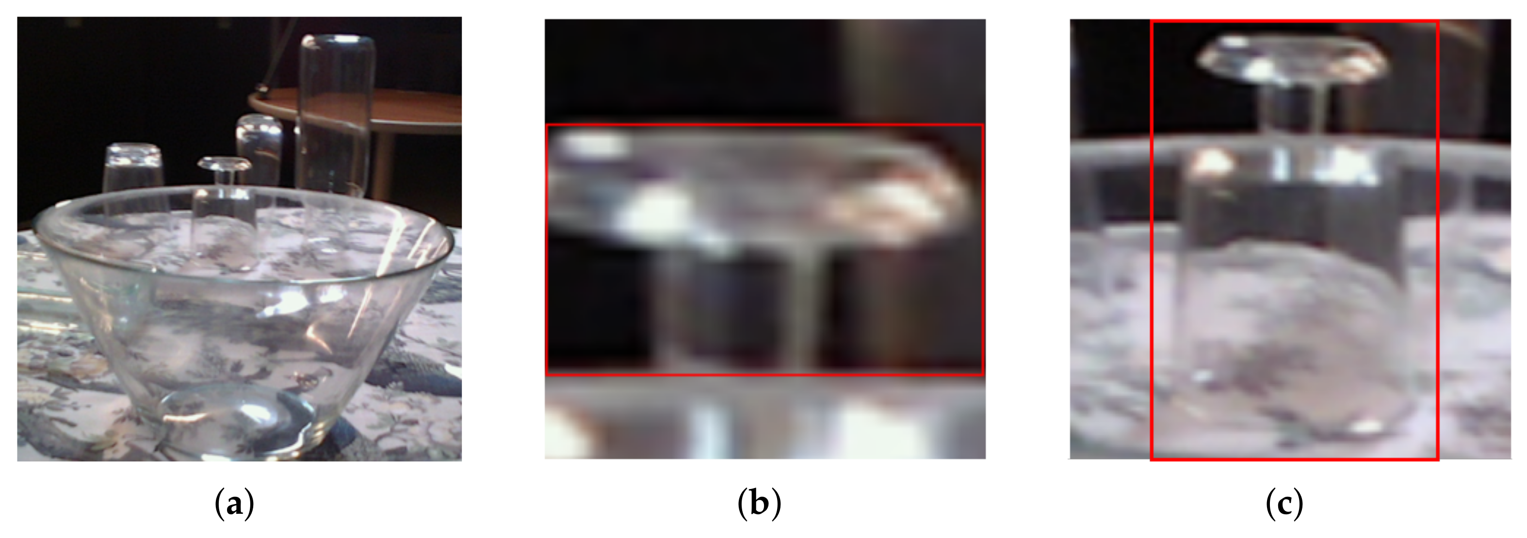
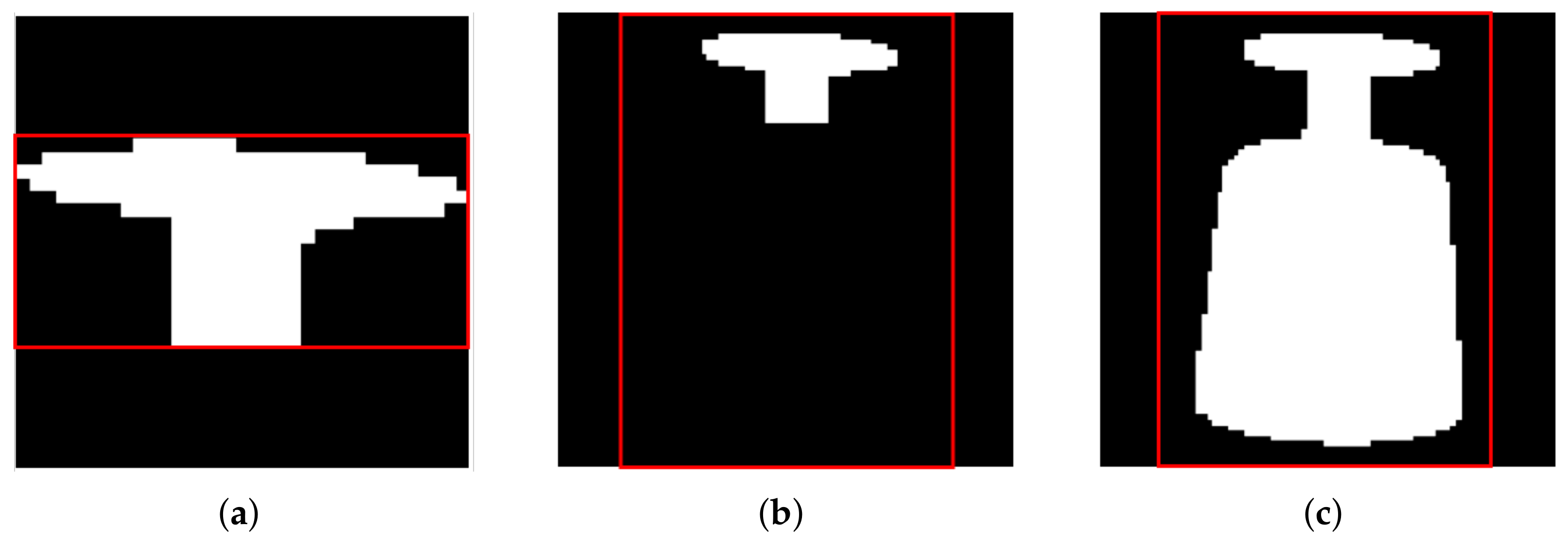
- modify ground-truth segmentation and bounding boxes to cover whole objects in cluttered transparent scenes,
- compare training with transparency-aware and original segmentation and its influence on the pose,
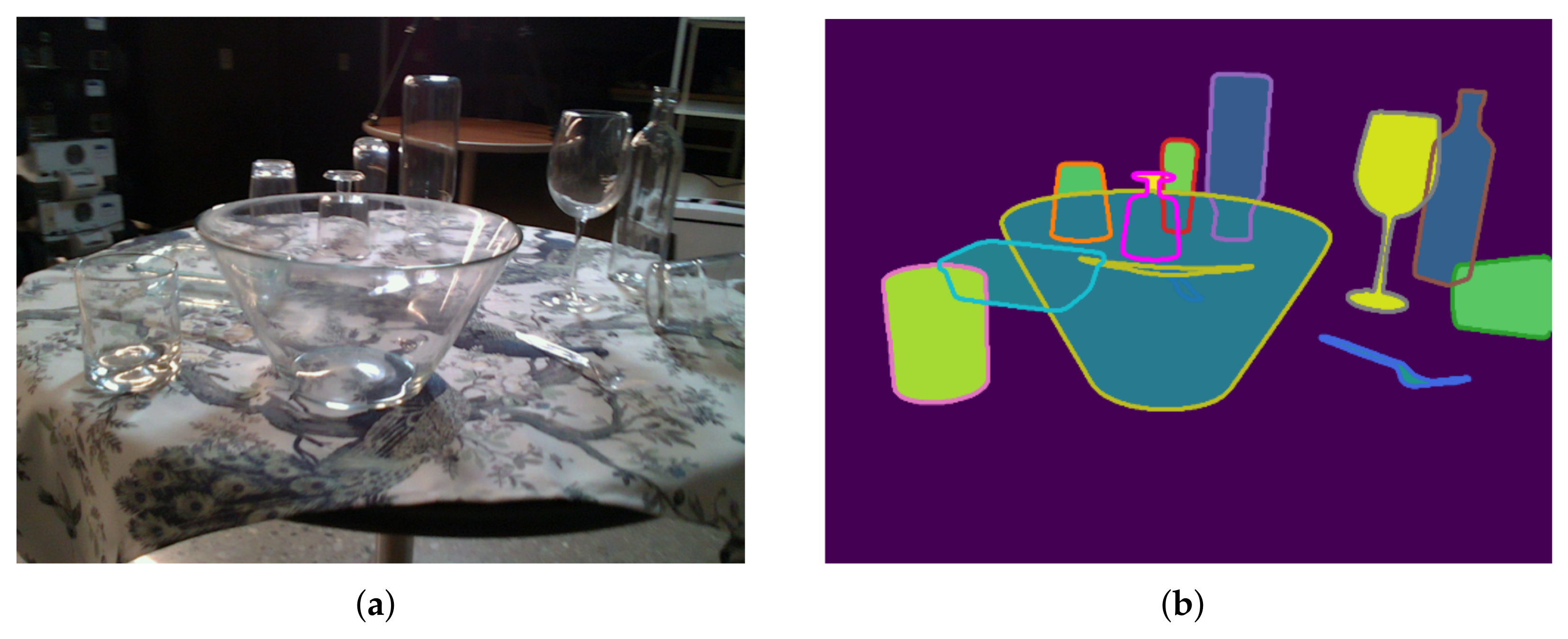
- apply our approach to a cluttered challenging glass scene using only RGB data without modifications specific to the glass dataset.
2. Related Work
3. Approach
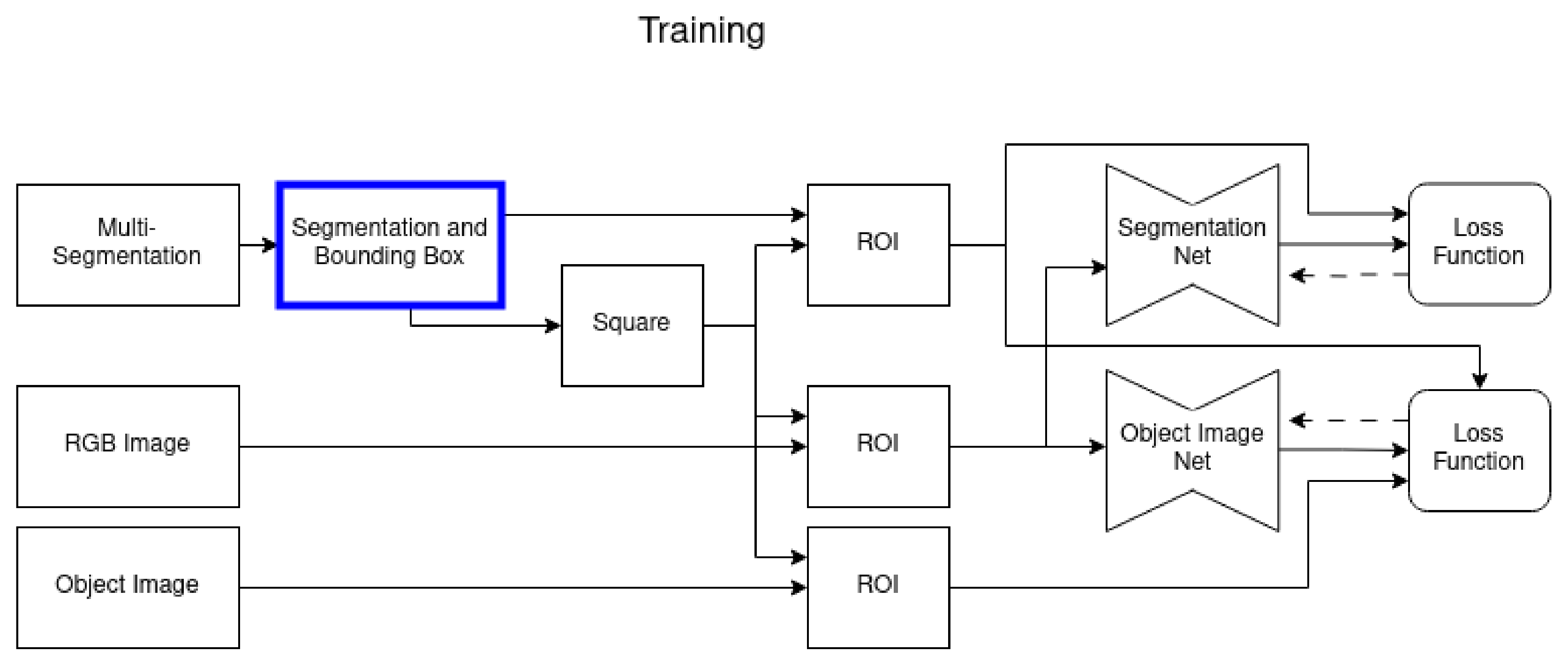
3.1. Training
3.2. Prediction
4. Dataset
5. Experiments
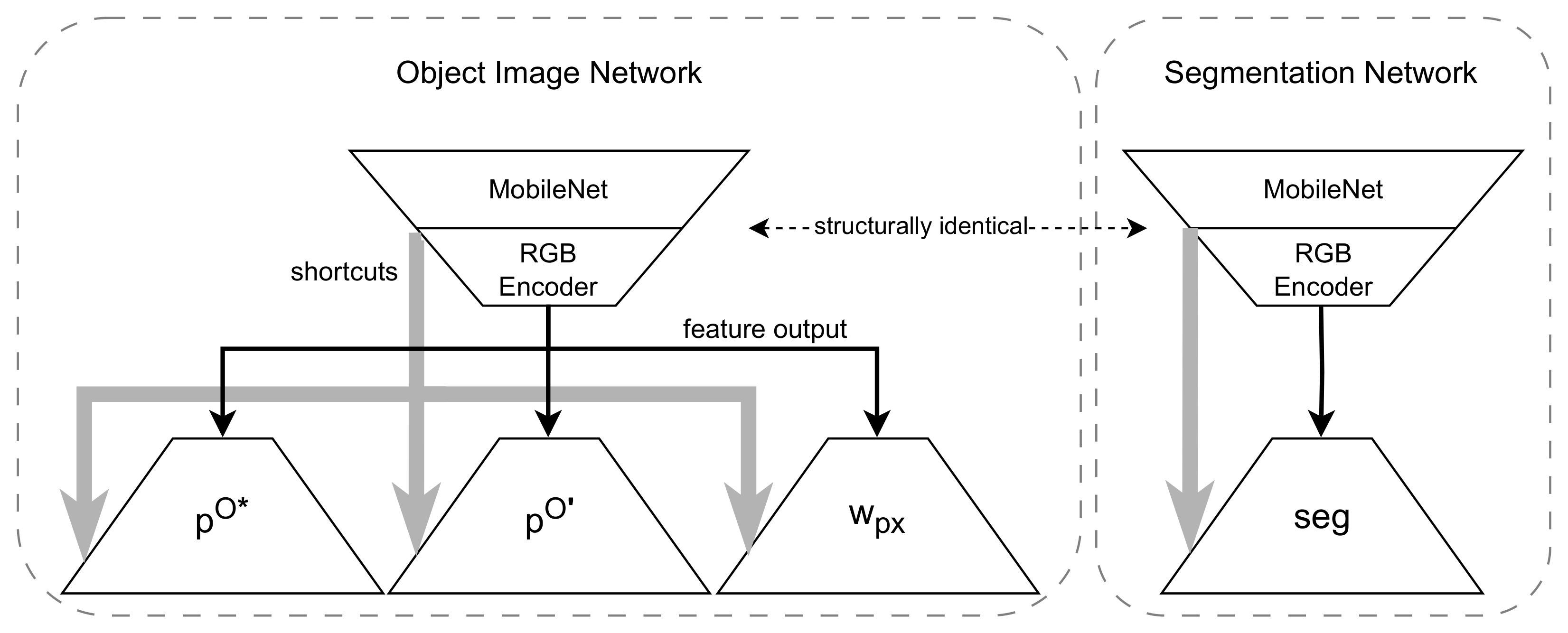
5.1. Network Architecture
5.2. Training
6. Results
6.1. Segmentation
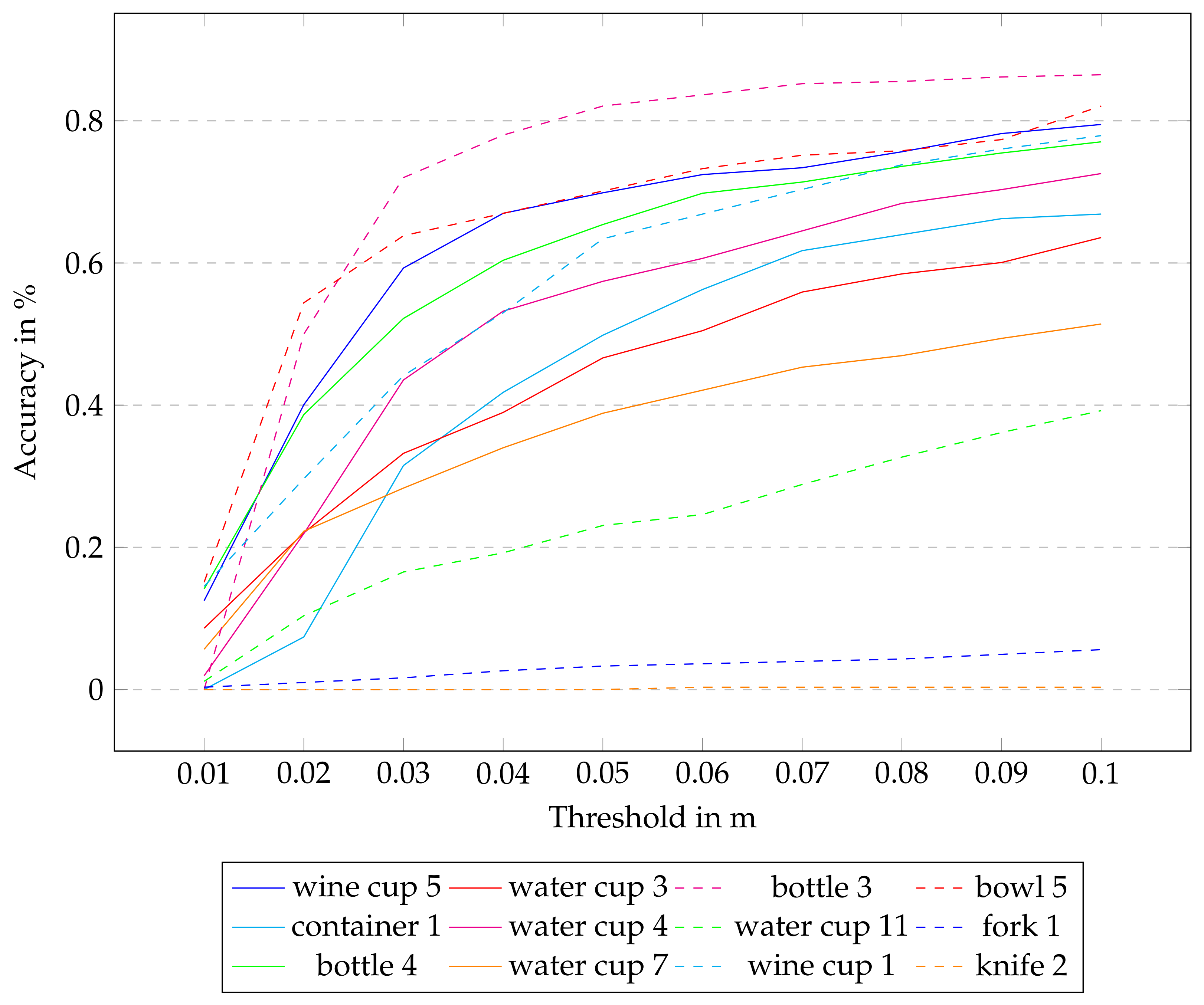
6.2. 6D Pose Estimation
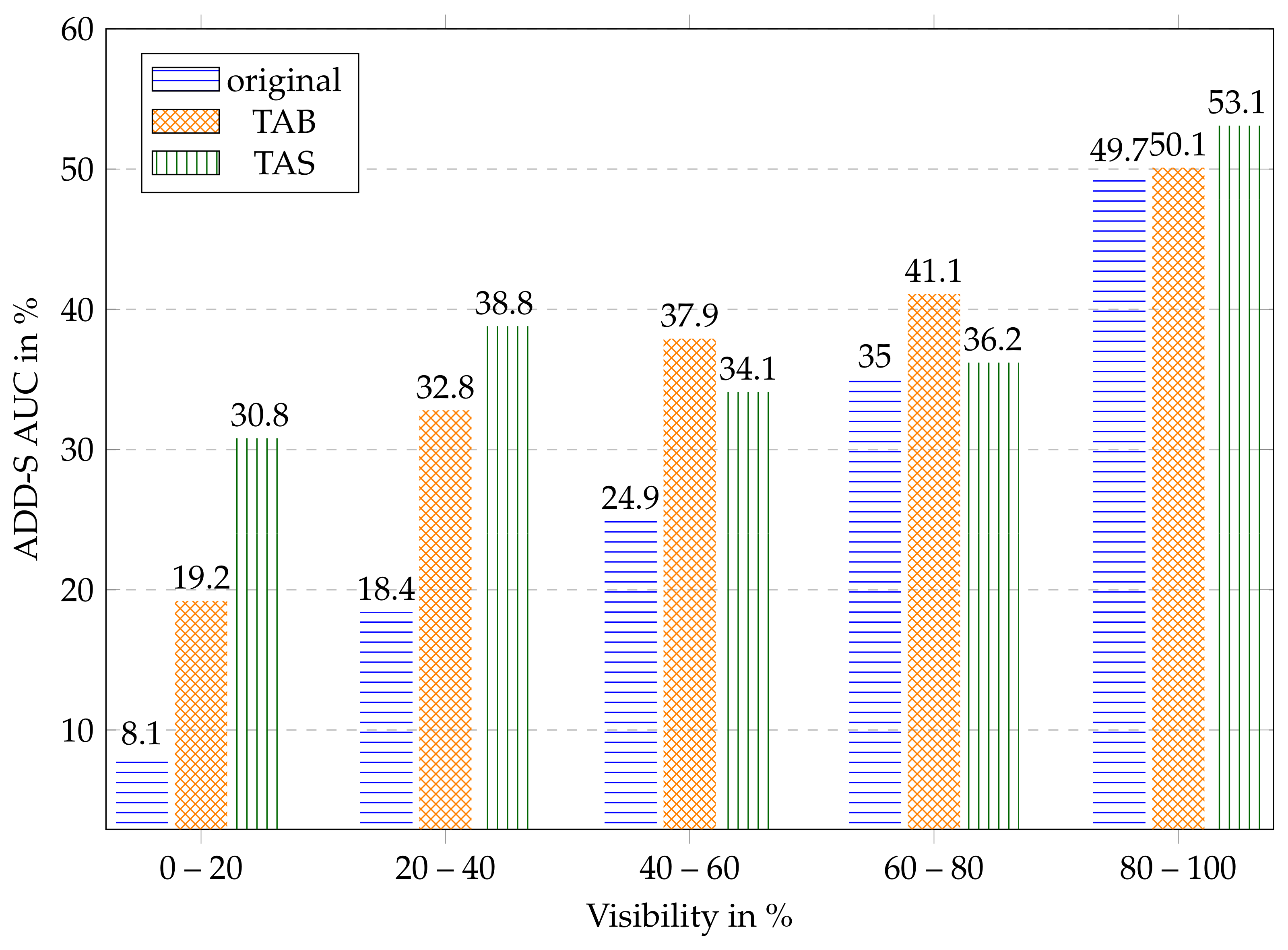
6.3. Dependence on Level of Occlusion
6.4. Knife and Fork
7. Conclusions
Author Contributions
Funding
Institutional Review Board Statement
Informed Consent Statement
Data Availability Statement
Conflicts of Interest
Abbreviations
| ADD-S | Symmetry-aware average point distance |
| AUC | Area under the curve |
| TAB | Transparency-aware bounding box |
| TAS | Transparency-aware segmentation |
| ROI | Region of interest |
References
- Su, Y.; Saleh, M.; Fetzer, T.; Rambach, J.; Navab, N.; Busam, B.; Stricker, D.; Tombari, F. ZebraPose: Coarse to Fine Surface Encoding for 6DoF Object Pose Estimation. arXiv 2022, arXiv:2203.09418. [Google Scholar]
- Park, K.; Patten, T.; Vincze, M. Pix2Pose: Pixel-Wise Coordinate Regression of Objects for 6D Pose Estimation. In Proceedings of the IEEE/CVF International Conference on Computer Vision (ICCV), Seoul, Republic of Korea, 27 October–2 November 2019. [Google Scholar]
- He, Y.; Huang, H.; Fan, H.; Chen, Q.; Sun, J. FFB6D: A Full Flow Bidirectional Fusion Network for 6D Pose Estimation. arXiv 2021, arXiv:2103.02242. [Google Scholar]
- Richter-Klug, J.; Frese, U. Towards Meaningful Uncertainty Information for CNN Based 6D Pose Estimates. In Proceedings of the Computer Vision Systems; Tzovaras, D., Giakoumis, D., Vincze, M., Argyros, A., Eds.; Springer: Cham, Switzerland, 2019; pp. 408–422. [Google Scholar]
- Wang, C.; Xu, D.; Zhu, Y.; Martin-Martin, R.; Lu, C.; Fei-Fei, L.; Savarese, S. DenseFusion: 6D Object Pose Estimation by Iterative Dense Fusion. In Proceedings of the IEEE/CVF Conference on Computer Vision and Pattern Recognition (CVPR), Long Beach, CA, USA, 15–20 June 2019. [Google Scholar]
- Labbé, Y.; Carpentier, J.; Aubry, M.; Sivic, J. CosyPose: Consistent multi-view multi-object 6D pose estimation. arXiv 2020, arXiv:2008.08465. [Google Scholar]
- Li, Y.; Wang, G.; Ji, X.; Xiang, Y.; Fox, D. DeepIM: Deep Iterative Matching for 6D Pose Estimation. Int. J. Comput. Vis. 2019, 128, 657–678. [Google Scholar] [CrossRef]
- Krull, A.; Brachmann, E.; Nowozin, S.; Michel, F.; Shotton, J.; Rother, C. PoseAgent: Budget-Constrained 6D Object Pose Estimation via Reinforcement Learning. In Proceedings of the IEEE Conference on Computer Vision and Pattern Recognition (CVPR), Honolulu, HI, USA, 21–26 July 2017. [Google Scholar]
- Rad, M.; Lepetit, V. BB8: A Scalable, Accurate, Robust to Partial Occlusion Method for Predicting the 3D Poses of Challenging Objects Without Using Depth. In Proceedings of the IEEE International Conference on Computer Vision (ICCV), Venice, Italy, 22–29 October 2017. [Google Scholar]
- Jiang, J.; Cao, G.; Do, T.T.; Luo, S. A4T: Hierarchical affordance detection for transparent objects depth reconstruction and manipulation. IEEE Robot. Autom. Lett. 2022, 7, 9826–9833. [Google Scholar] [CrossRef]
- Xu, C.; Chen, J.; Yao, M.; Zhou, J.; Zhang, L.; Liu, Y. 6DoF Pose Estimation of Transparent Object from a Single RGB-D Image. Sensors 2020, 20, 6790. [Google Scholar] [CrossRef] [PubMed]
- Tang, Y.; Chen, J.; Yang, Z.; Lin, Z.; Li, Q.; Liu, W. DepthGrasp: Depth Completion of Transparent Objects Using Self-Attentive Adversarial Network with Spectral Residual for Grasping. In Proceedings of the 2021 IEEE/RSJ International Conference on Intelligent Robots and Systems (IROS), Prague, Czech Republic, 27 September–1 October 2021; pp. 5710–5716. [Google Scholar] [CrossRef]
- Liu, X.; Jonschkowski, R.; Angelova, A.; Konolige, K. Keypose: Multi-view 3d labeling and keypoint estimation for transparent objects. In Proceedings of the IEEE/CVF Conference on Computer Vision and Pattern Recognition, Seattle, WA, USA, 14–19 June 2020; pp. 11602–11610. [Google Scholar]
- Yu, H.; Li, S.; Liu, H.; Xia, C.; Ding, W.; Liang, B. TGF-Net: Sim2Real Transparent Object 6D Pose Estimation Based on Geometric Fusion. IEEE Robot. Autom. Lett. 2023, 8, 3868–3875. [Google Scholar] [CrossRef]
- Byambaa, M.; Koutaki, G.; Choimaa, L. 6D Pose Estimation of Transparent Object From Single RGB Image for Robotic Manipulation. IEEE Access 2022, 10, 114897–114906. [Google Scholar] [CrossRef]
- Chen, X.; Zhang, H.; Yu, Z.; Opipari, A.; Jenkins, O.C. ClearPose: Large-scale Transparent Object Dataset and Benchmark. arXiv 2022, arXiv:2203.03890. [Google Scholar]
- Kendall, A.; Grimes, M.; Cipolla, R. PoseNet: A Convolutional Network for Real-Time 6-DOF Camera Relocalization. arXiv 2016, arXiv:1505.07427. [Google Scholar]
- Wang, G.; Manhardt, F.; Tombari, F.; Ji, X. GDR-Net: Geometry-Guided Direct Regression Network for Monocular 6D Object Pose Estimation. arXiv 2021, arXiv:2102.12145. [Google Scholar]
- Richter-Klug, J.; Frese, U. Handling Object Symmetries in CNN-based Pose Estimation. In Proceedings of the 2021 IEEE International Conference on Robotics and Automation (ICRA), Xi’an, China, 30 May–5 June 2021; pp. 13850–13856. [Google Scholar] [CrossRef]
- Redmon, J.; Divvala, S.; Girshick, R.; Farhadi, A. You Only Look Once: Unified, Real-Time Object Detection. In Proceedings of the 2016 IEEE Conference on Computer Vision and Pattern Recognition (CVPR), Las Vegas, NV, USA, 27–30 June 2016; pp. 779–788. [Google Scholar] [CrossRef]
- Ren, S.; He, K.; Girshick, R.; Sun, J. Faster R-CNN: Towards Real-Time Object Detection with Region Proposal Networks. arXiv 2016, arXiv:1506.01497. [Google Scholar] [CrossRef] [PubMed]
- Tan, M.; Pang, R.; Le, Q.V. EfficientDet: Scalable and Efficient Object Detection. In Proceedings of the IEEE/CVF Conference on Computer Vision and Pattern Recognition (CVPR), Seattle, WA, USA, 14–19 June 2020. [Google Scholar]
- Zand, M.; Etemad, A.; Greenspan, M. Oriented Bounding Boxes for Small and Freely Rotated Objects. IEEE Trans. Geosci. Remote Sens. 2022, 60, 1–15. [Google Scholar] [CrossRef]
- Yang, X.; Yang, J.; Yan, J.; Zhang, Y.; Zhang, T.; Guo, Z.; Xian, S.; Fu, K. SCRDet: Towards More Robust Detection for Small, Cluttered and Rotated Objects. arXiv 2019, arXiv:1811.07126. [Google Scholar]
- Duan, K.; Bai, S.; Xie, L.; Qi, H.; Huang, Q.; Tian, Q. CenterNet: Keypoint Triplets for Object Detection. In Proceedings of the IEEE/CVF International Conference on Computer Vision (ICCV), Seoul, Republic of Korea, 27 October–2 November 2019. [Google Scholar]
- Yoo, D.; Park, S.; Lee, J.Y.; Paek, A.S.; Kweon, I.S. AttentionNet: Aggregating Weak Directions for Accurate Object Detection. In Proceedings of the 2015 IEEE International Conference on Computer Vision (ICCV), Santiago, Chile, 7–13 December 2015; pp. 2659–2667. [Google Scholar] [CrossRef]
- Sajjan, S.S.; Moore, M.; Pan, M.; Nagaraja, G.; Lee, J.; Zeng, A.; Song, S. ClearGrasp: 3D Shape Estimation of Transparent Objects for Manipulation. arXiv 2019, arXiv:1910.02550. [Google Scholar]
- Fang, H.; Fang, H.S.; Xu, S.; Lu, C. TransCG: A Large-Scale Real-World Dataset for Transparent Object Depth Completion and a Grasping Baseline. IEEE Robot. Autom. Lett. 2022, 7, 7383–7390. [Google Scholar] [CrossRef]
- Xiang, Y.; Schmidt, T.; Narayanan, V.; Fox, D. PoseCNN: A Convolutional Neural Network for 6D Object Pose Estimation in Cluttered Scenes. arXiv 2018, arXiv:1711.00199. [Google Scholar]


| Layer Name | Nr. of Output Channels | Filter Size | Stride | Output Size | Nr. of Layers |
|---|---|---|---|---|---|
| MN block_3_project_BN | 32 | - | - | 28 × 28 | - |
| Conv1 | 100 | 5 × 5 | 2 | 14 × 14 | 1 |
| Dense1 | 64 | - | 1 | 14 × 14 | 12 × 3 |
| Conv2 | 128 | 1 × 1 | 1 | 14 × 14 | 1 |
| Dense2 | 64 | - | 1 | 14 × 14 | 12 × 3 |
| Conv3 | 128 | 1 × 1 | 1 | 14 × 14 | 1 |
| Conv4 | 70 | 5 × 5 | 2 | 7 × 7 | 1 |
| Dense3 | 70 | - | 1 | 7 × 7 | 6 × 3 |
| Conv5 | 140 | 1 × 1 | 1 | 7 × 7 | 1 |
| Layer Name | Nr. of Output Channels | Filter Size | Stride | Output Size | Nr. of Layers |
|---|---|---|---|---|---|
| Up1 | 140 | - | - | 14 × 14 | 1 |
| Concat2 | 268 | Conv3 (Enc.) & Conv5 (Enc.) | 14 × 14 | 1 | |
| Conv6 | 50 | 3 × 3 | 1 | 14 × 14 | 1 |
| Dense4 | 25 | - | 1 | 14 × 14 | 12 × 3 |
| Conv7 | 50 | 1 × 1 | 1 | 14 × 14 | 1 |
| Up2 | 50 | - | - | 28 × 28 | 1 |
| Concat3 | 82 | Dense4 & MN block_3_project_BN | 28 × 28 | 1 | |
| Conv8 | 32 | 3 × 3 | 1 | 28 × 28 | 1 |
| Dense5 | 16 | - | 1 | 28 × 28 | 6 × 3 |
| Conv9 | 32 | 1 × 1 | 1 | 28 × 28 | 1 |
| Up3 | 32 | - | - | 56 × 56 | 1 |
| Concat4 | 56 | Dense5 & MN block_2_project_BN | 56 × 56 | 1 | |
| Conv10 | 24 | 3 × 3 | 1 | 56 × 56 | 1 |
| Dense6 | 12 | - | 1 | 56 × 56 | 4 × 3 |
| Conv11 | 24 | 1 × 1 | 1 | 56 × 56 | 1 |
| Up4 | 24 | - | - | 112 × 112 | 1 |
| Concat5 | 56 | Dense6 & MN bn_Conv1 | 112 × 112 | 1 | |
| Conv12 | 16 | 3 × 3 | 1 | 112 × 112 | 1 |
| Dense7 | 8 | - | 1 | 112 × 112 | 4 × 3 |
| Conv13 | 16 | 1 × 1 | 1 | 112 × 112 | 1 |
| Conv (///seg) | 3/3/4/1 | 1 × 1 | 1 | 112 × 112 | 1 |
| Layer Name | Nr. of Output Channels | Filter Size | Stride | Output Size | Nr. of Layers |
|---|---|---|---|---|---|
| ConvI | input channels | 1 × 1 | 1 | input size | 1 |
| ConvII | input channels | 3 × 3 | 1 | input size | 1 |
| Concat | Input Layer & ConvII | input size | 1 | ||
| Original | TAB | TAS | |
|---|---|---|---|
| recall | 83.64% | 79.13% | 89.53% |
| precision | 93.10% | 93.82% | 97.22% |
Disclaimer/Publisher’s Note: The statements, opinions and data contained in all publications are solely those of the individual author(s) and contributor(s) and not of MDPI and/or the editor(s). MDPI and/or the editor(s) disclaim responsibility for any injury to people or property resulting from any ideas, methods, instructions or products referred to in the content. |
© 2024 by the authors. Licensee MDPI, Basel, Switzerland. This article is an open access article distributed under the terms and conditions of the Creative Commons Attribution (CC BY) license (https://creativecommons.org/licenses/by/4.0/).
Share and Cite
Weidenbach, M.; Laue, T.; Frese, U. Transparency-Aware Segmentation of Glass Objects to Train RGB-Based Pose Estimators. Sensors 2024, 24, 432. https://doi.org/10.3390/s24020432
Weidenbach M, Laue T, Frese U. Transparency-Aware Segmentation of Glass Objects to Train RGB-Based Pose Estimators. Sensors. 2024; 24(2):432. https://doi.org/10.3390/s24020432
Chicago/Turabian StyleWeidenbach, Maira, Tim Laue, and Udo Frese. 2024. "Transparency-Aware Segmentation of Glass Objects to Train RGB-Based Pose Estimators" Sensors 24, no. 2: 432. https://doi.org/10.3390/s24020432
APA StyleWeidenbach, M., Laue, T., & Frese, U. (2024). Transparency-Aware Segmentation of Glass Objects to Train RGB-Based Pose Estimators. Sensors, 24(2), 432. https://doi.org/10.3390/s24020432