Author Contributions
Conceptualization, S.N.G.; methodology, M.P.K. and V.D.G.; software, A.N.P. and E.A.O.; validation, E.A.O. and E.S.M.; formal analysis, E.A.O. and V.D.G.; investigation, M.P.K. and A.N.P.; resources, E.S.M. and V.D.G.; data curation, M.P.K., A.A.O. and A.N.P.; writing—original draft preparation, M.P.K. and A.A.O.; writing—review and editing, M.P.K. and S.N.G.; visualization, E.S.M., A.A.O. and A.N.P.; supervision, S.N.G.; project administration, M.P.K.; funding acquisition, S.N.G. All authors have read and agreed to the published version of the manuscript.
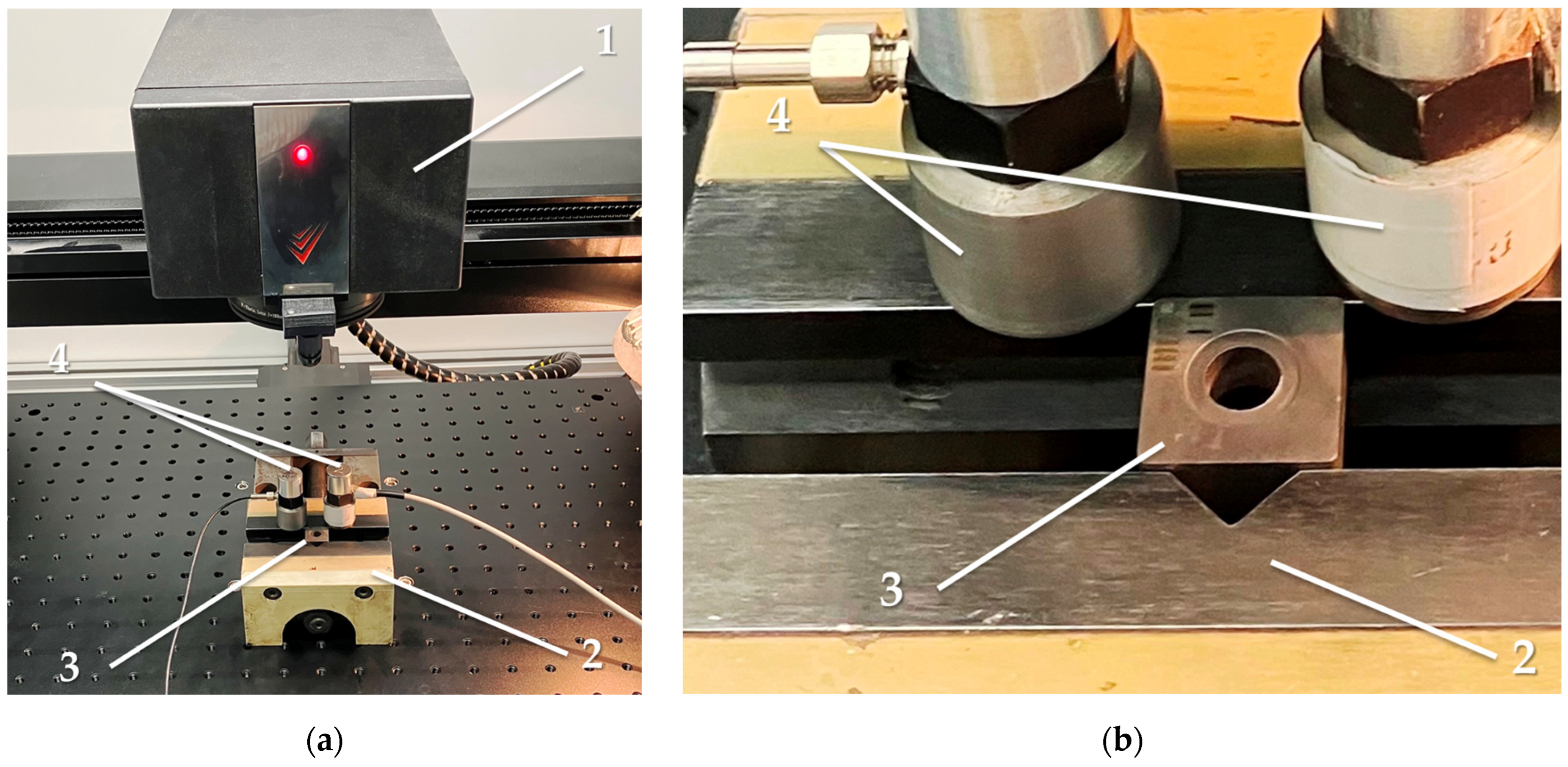
Figure 1.
Laser processing machine, SharpMark Fiber GT 60: (a) general view of the working area; (b) cutting insert made of the hard alloy T15K6 in a vice and accelerometers, where (1) is a laser module, (2) is a vice, (3) is a fastened workpiece, and (4) shows accelerometers.
Figure 1.
Laser processing machine, SharpMark Fiber GT 60: (a) general view of the working area; (b) cutting insert made of the hard alloy T15K6 in a vice and accelerometers, where (1) is a laser module, (2) is a vice, (3) is a fastened workpiece, and (4) shows accelerometers.
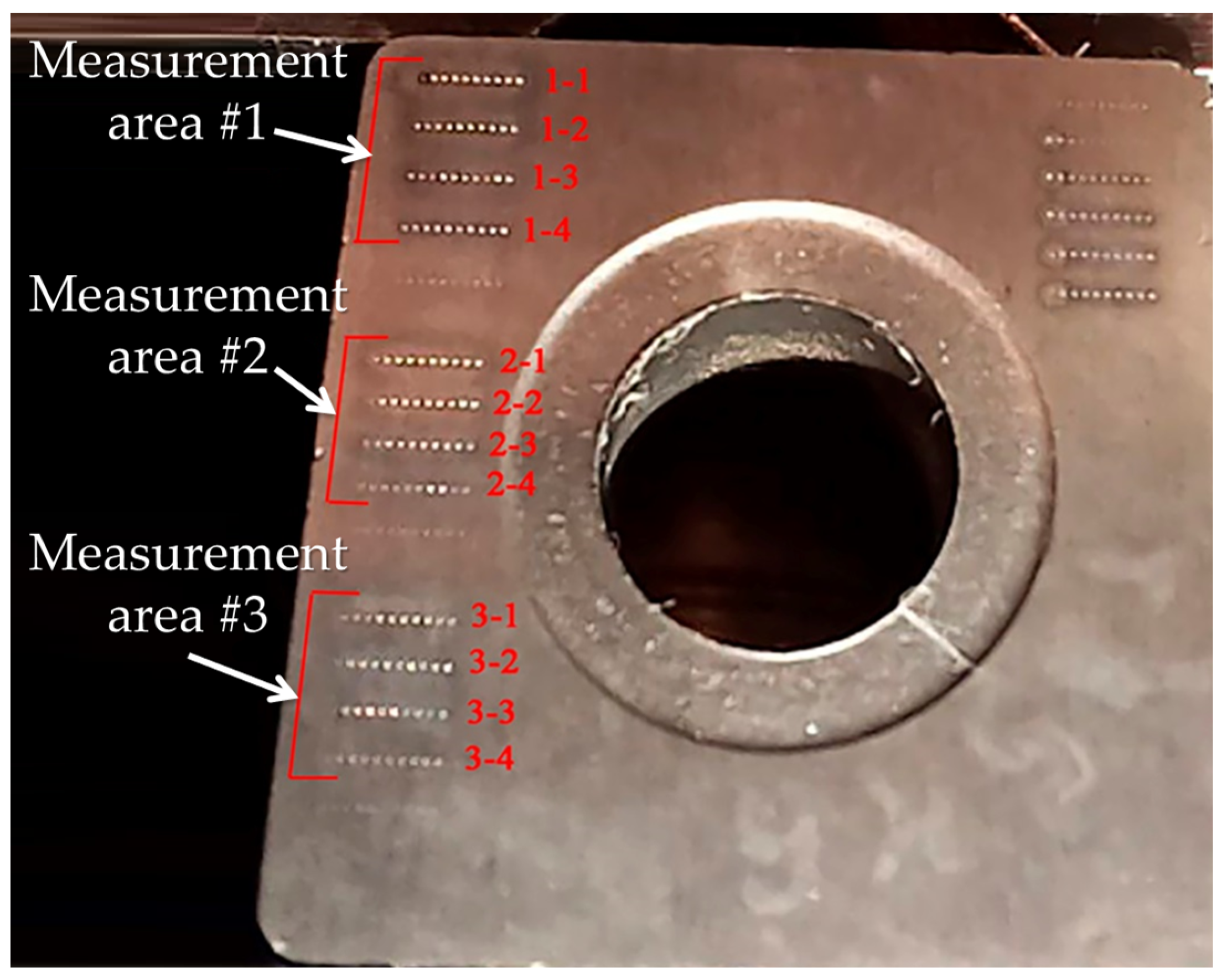
Figure 2.
The general view of cutting insert made of T15K6 alloy.
Figure 2.
The general view of cutting insert made of T15K6 alloy.
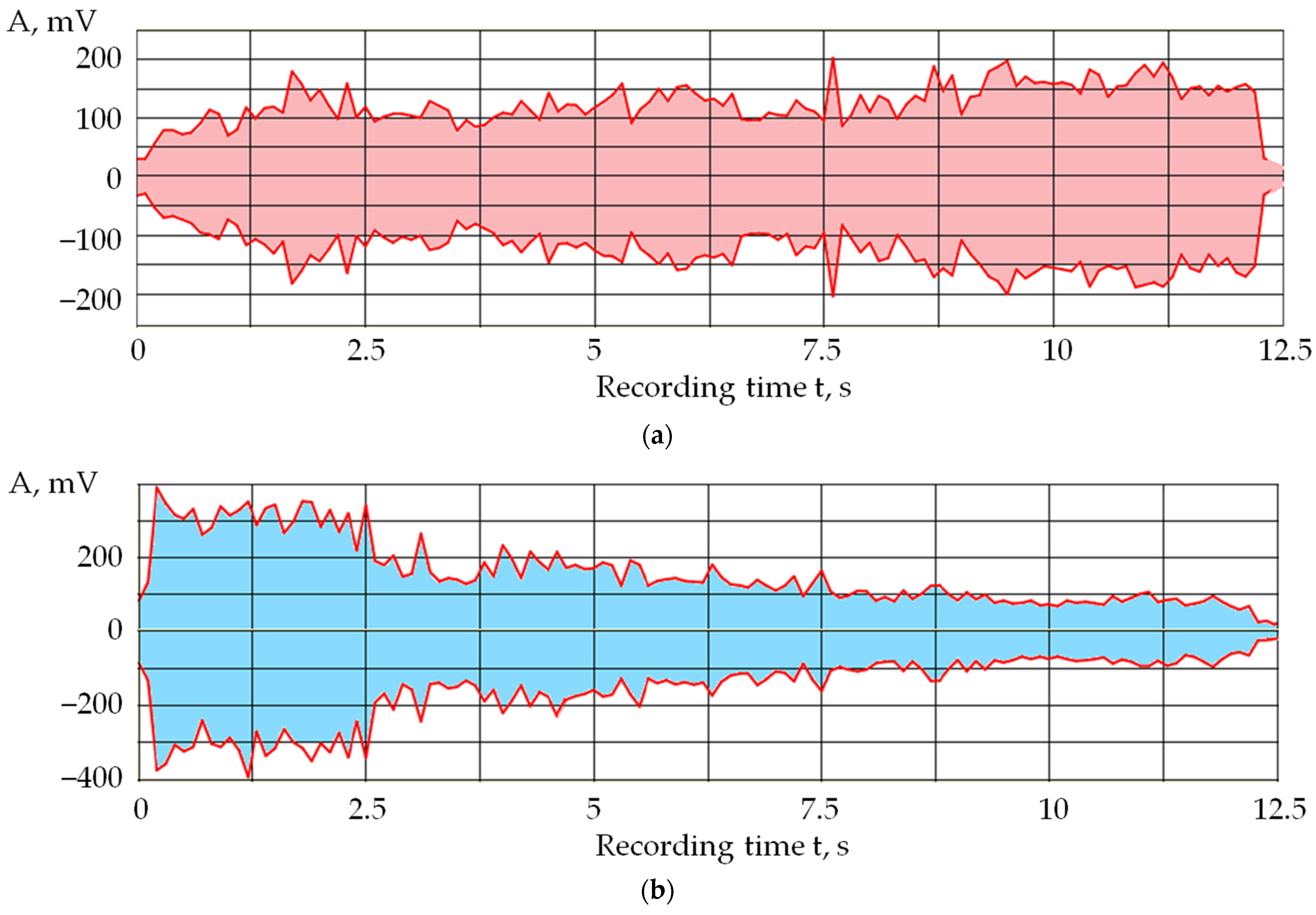
Figure 3.
Envelopes of acoustic emission signals in two frequency ranges from the moment the electrical discharge machining begins until the wire electrode breaks: (a) low-frequency range; (b) high-frequency range.
Figure 3.
Envelopes of acoustic emission signals in two frequency ranges from the moment the electrical discharge machining begins until the wire electrode breaks: (a) low-frequency range; (b) high-frequency range.
Figure 4.
Formation of various regions when laser pulses act on the surface of a substance: (1) is a region of elastic deformations; (2) is a plastic deformation region; (3) is melt; (4) is vapors of matter; (5) is plasma; (6) is laser beam.
Figure 4.
Formation of various regions when laser pulses act on the surface of a substance: (1) is a region of elastic deformations; (2) is a plastic deformation region; (3) is melt; (4) is vapors of matter; (5) is plasma; (6) is laser beam.
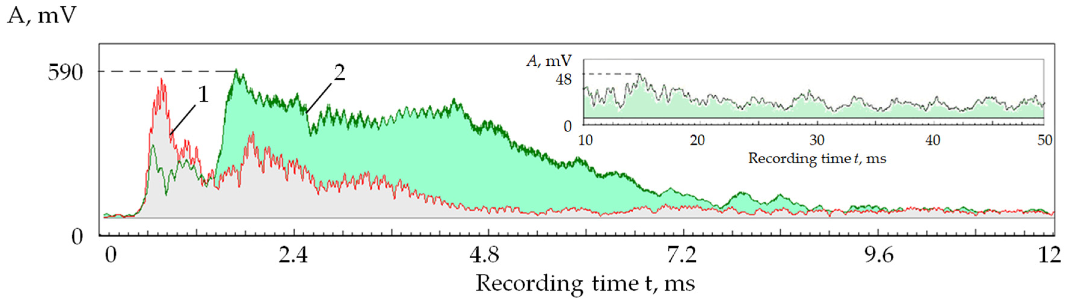
Figure 5.
Interaction of laser pulses with the T15K6 alloy and its display in acoustic emission signals: RMS amplitude of the acoustic emission signal in the frequency ranges 5–17 kHz (1) and 35–50 kHz (2); inset shows the change in RMS amplitude in the range of 35–50 kHz after the 10th ms.
Figure 5.
Interaction of laser pulses with the T15K6 alloy and its display in acoustic emission signals: RMS amplitude of the acoustic emission signal in the frequency ranges 5–17 kHz (1) and 35–50 kHz (2); inset shows the change in RMS amplitude in the range of 35–50 kHz after the 10th ms.
Figure 6.
RMS amplitude of the acoustic emission signal in 5–17 kHz when sequentially applying laser pulses to 24 points in 50 passes (pulse frequency of 2 kHz ≈ interval of 12 ms).
Figure 6.
RMS amplitude of the acoustic emission signal in 5–17 kHz when sequentially applying laser pulses to 24 points in 50 passes (pulse frequency of 2 kHz ≈ interval of 12 ms).
Figure 7.
RMS amplitude of the acoustic emission signal in 5–17 kHz (1) and 35–50 kHz (2) when sequentially applying pulses to 24 points in 50 passes.
Figure 7.
RMS amplitude of the acoustic emission signal in 5–17 kHz (1) and 35–50 kHz (2) when sequentially applying pulses to 24 points in 50 passes.
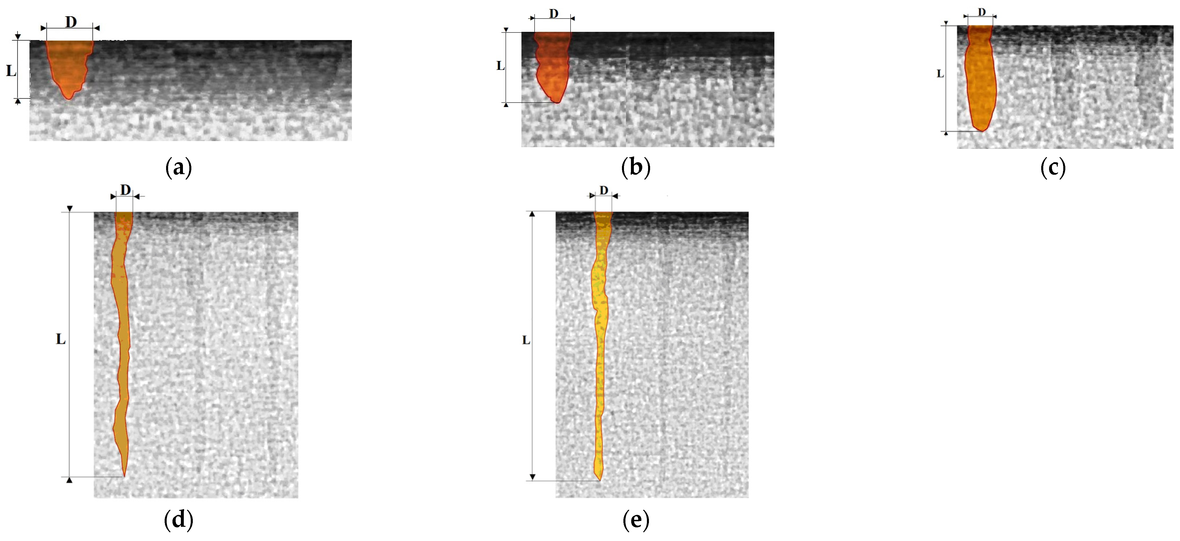
Figure 8.
Well profiles obtained on a tomograph FILIN CT-1500 after exposure to different numbers of laser pulses: (a) 5 pulses; (b) 10 pulses; (c) 20 pulses; (d) 40 pulses; (e) 80 pulses.
Figure 8.
Well profiles obtained on a tomograph FILIN CT-1500 after exposure to different numbers of laser pulses: (a) 5 pulses; (b) 10 pulses; (c) 20 pulses; (d) 40 pulses; (e) 80 pulses.
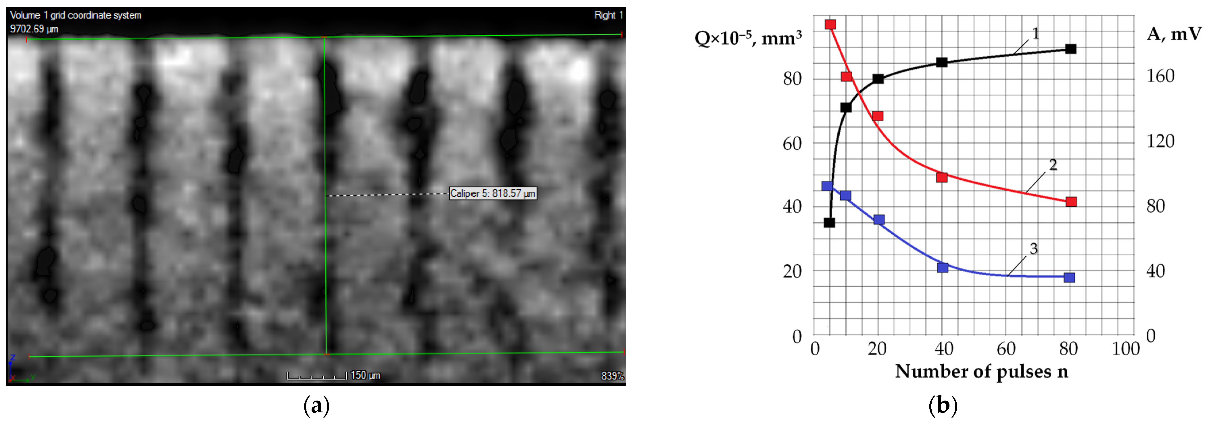
Figure 9.
The wells on the tomograph (a) and the dependence of the volume of the wells and the RMS amplitudes of the acoustic emission signals during processing with different numbers of pulses (b): 1 is the volume of the wells Q with a different number of pulses; 2 is RMS amplitude of acoustic emission in the range of 5–17 kHz; 3 is RMS amplitude of acoustic emission in the range of 35–70 kHz.
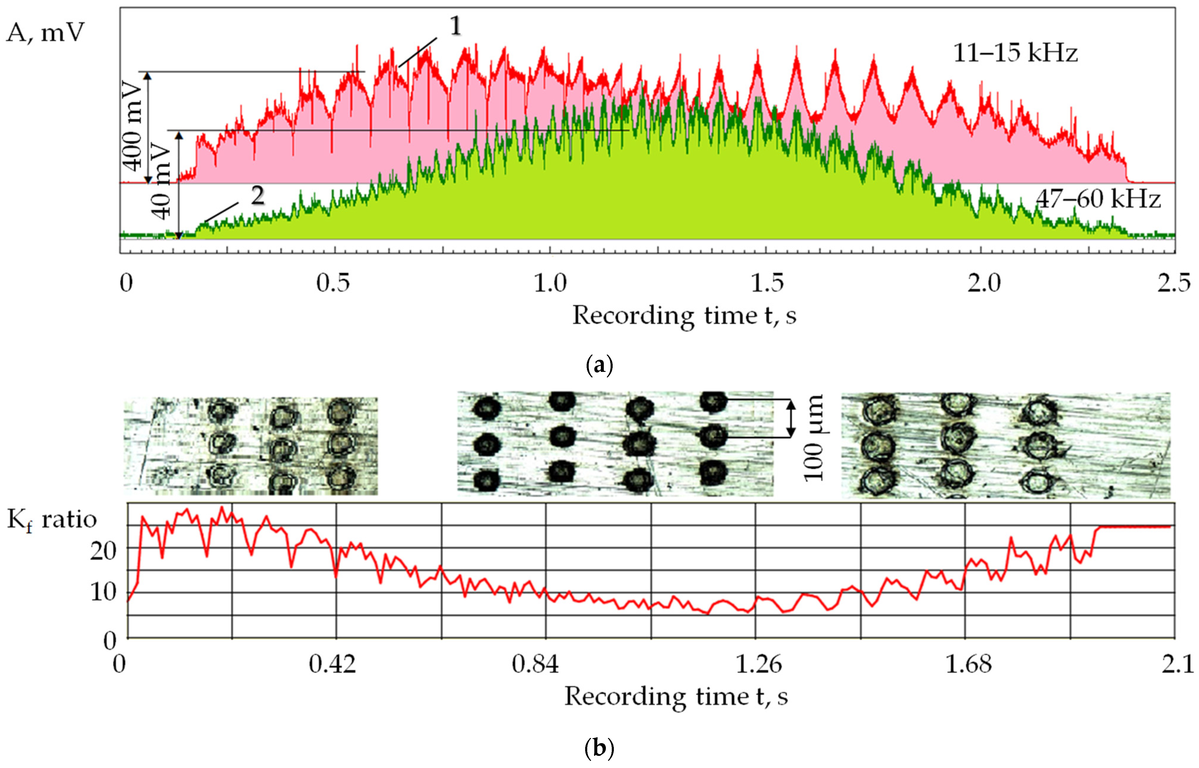
Figure 10.
Acoustic emission signals when processing a plate made of R6M5 high-speed steel installed with an inclination relative to the focal plane: (
a) RMS amplitudes in the ranges of 11–15 kHz (1) and 47–60 kHz (2); (
b) the ratio of RMS amplitudes 1 and 2 (K
f parameter) when displacement of the focal plane is above and below the processing surface, ∆ = ±1 mm (pictures in
Figure 10b show traces of laser pulses on different parts of the surface).
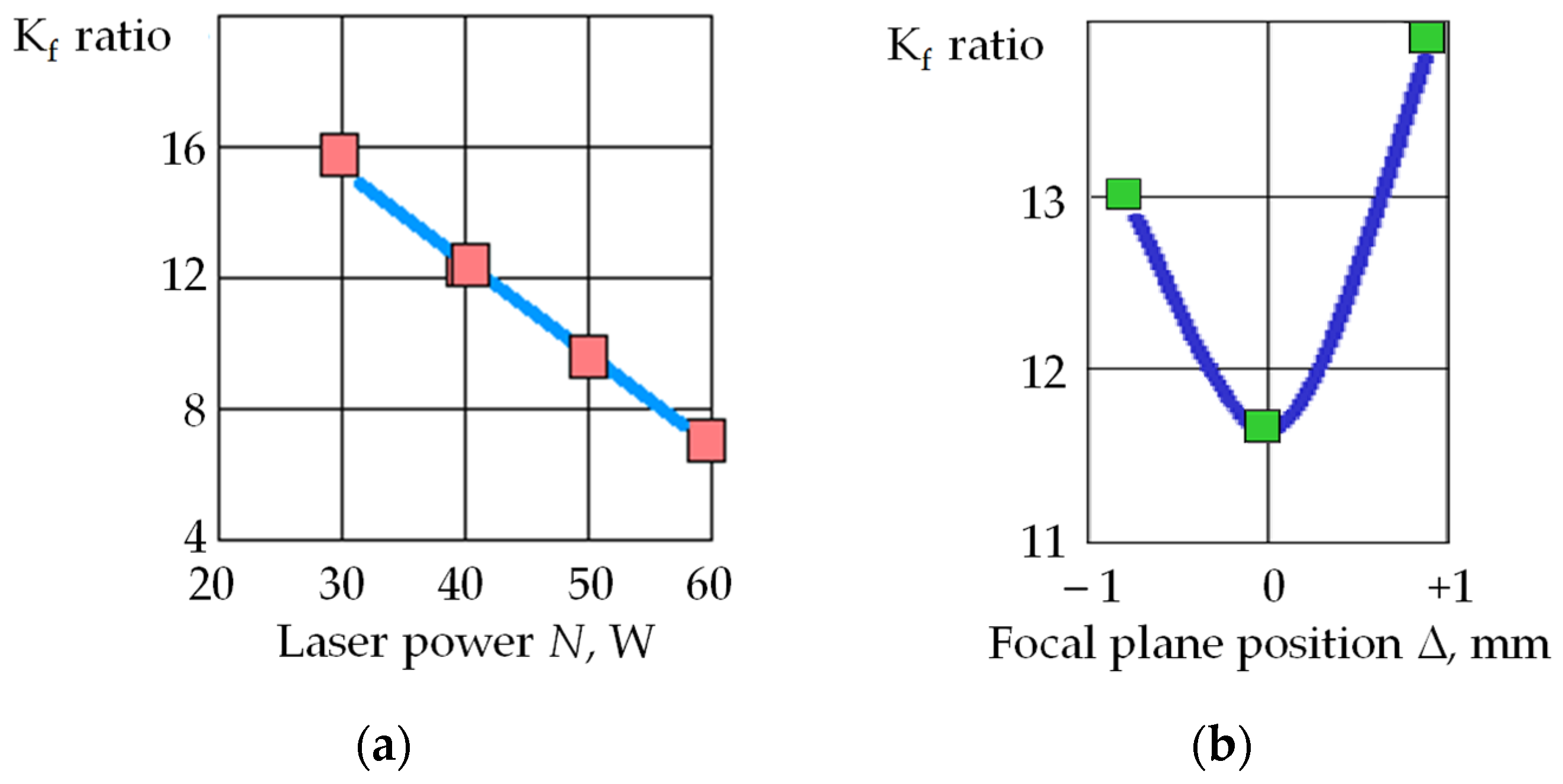
Figure 11.
The ratio of RMS amplitudes (Kf parameter) of acoustic emission signals in the ranges of 3–23 kHz and 31–51 kHz in D16 aluminum alloy processing: (a) to the power of laser pulses N, W; (b) to the position of the focal plane ∆, mm.
Figure 11.
The ratio of RMS amplitudes (Kf parameter) of acoustic emission signals in the ranges of 3–23 kHz and 31–51 kHz in D16 aluminum alloy processing: (a) to the power of laser pulses N, W; (b) to the position of the focal plane ∆, mm.
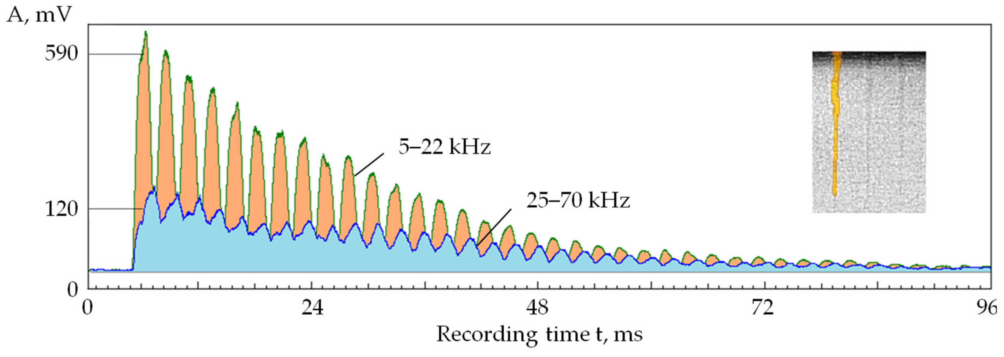
Figure 12.
RMS amplitudes of the acoustic emission signal in two frequency ranges when producing a line of 15 holes with the sequential supply of pulses in 80 passes (the first microseconds of the recording).
Figure 12.
RMS amplitudes of the acoustic emission signal in two frequency ranges when producing a line of 15 holes with the sequential supply of pulses in 80 passes (the first microseconds of the recording).
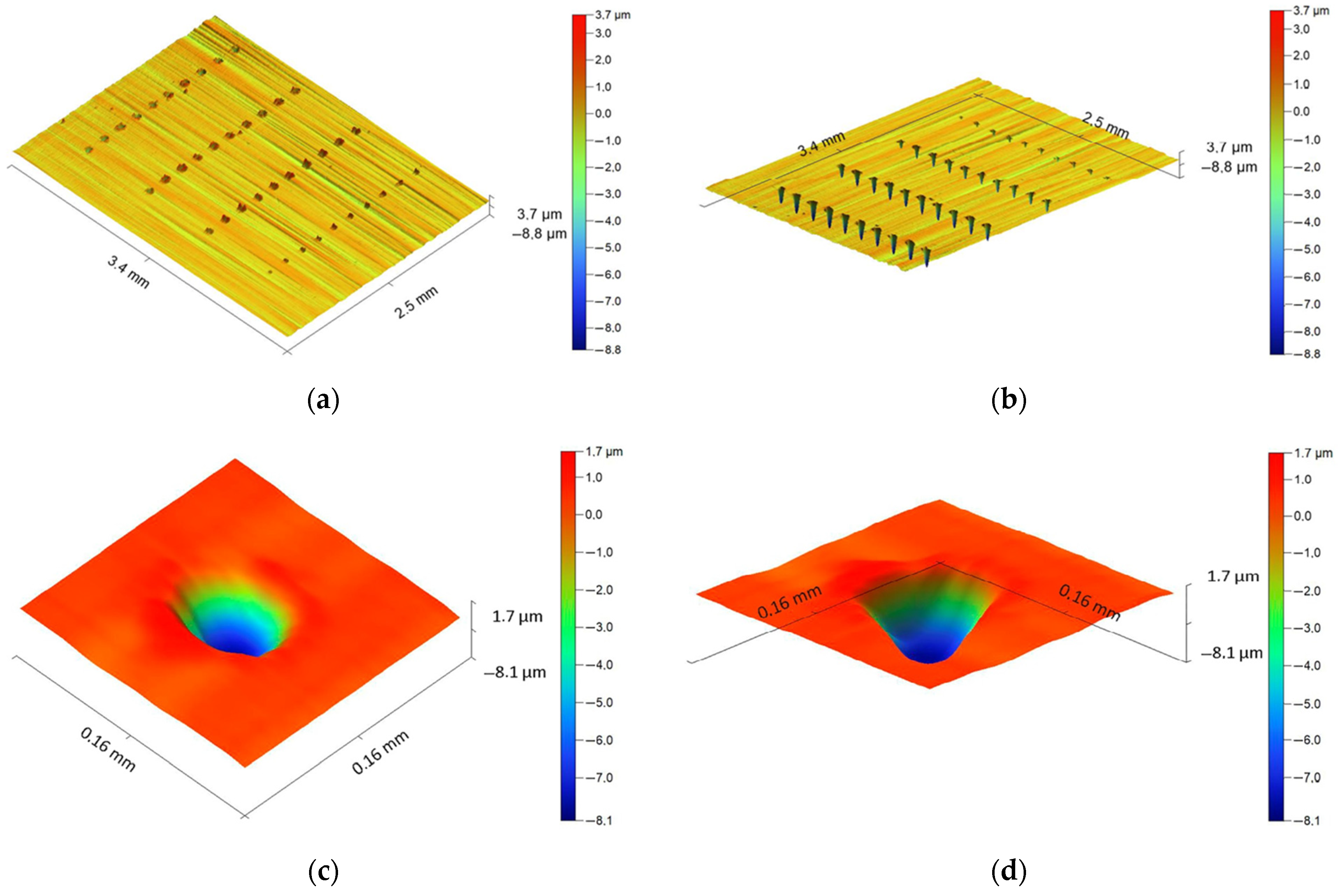
Figure 13.
Well profiles on the surface of T15K6 cutting insert obtained using the Dektak XT stylus profilometer: (a) 3D profilogram (area 3, top view); (b) 3D profilogram (area 3, bottom view); (c) 3D profilogram (area 3-1, top view); (d) 3D profilogram of a well of (area 3-1, bottom view); (e) linear profilogram (mode 11); (f) linear profilogram (mode 14).
Figure 14.
The dependence of RMS amplitude of the acoustic emission signal in the low-frequency range (10–28 kHz, A1) on the power (N) and pulse duration (τ): (a) general view; (b–d) projections of lines of equal level onto coordinate planes.
Figure 14.
The dependence of RMS amplitude of the acoustic emission signal in the low-frequency range (10–28 kHz, A1) on the power (N) and pulse duration (τ): (a) general view; (b–d) projections of lines of equal level onto coordinate planes.
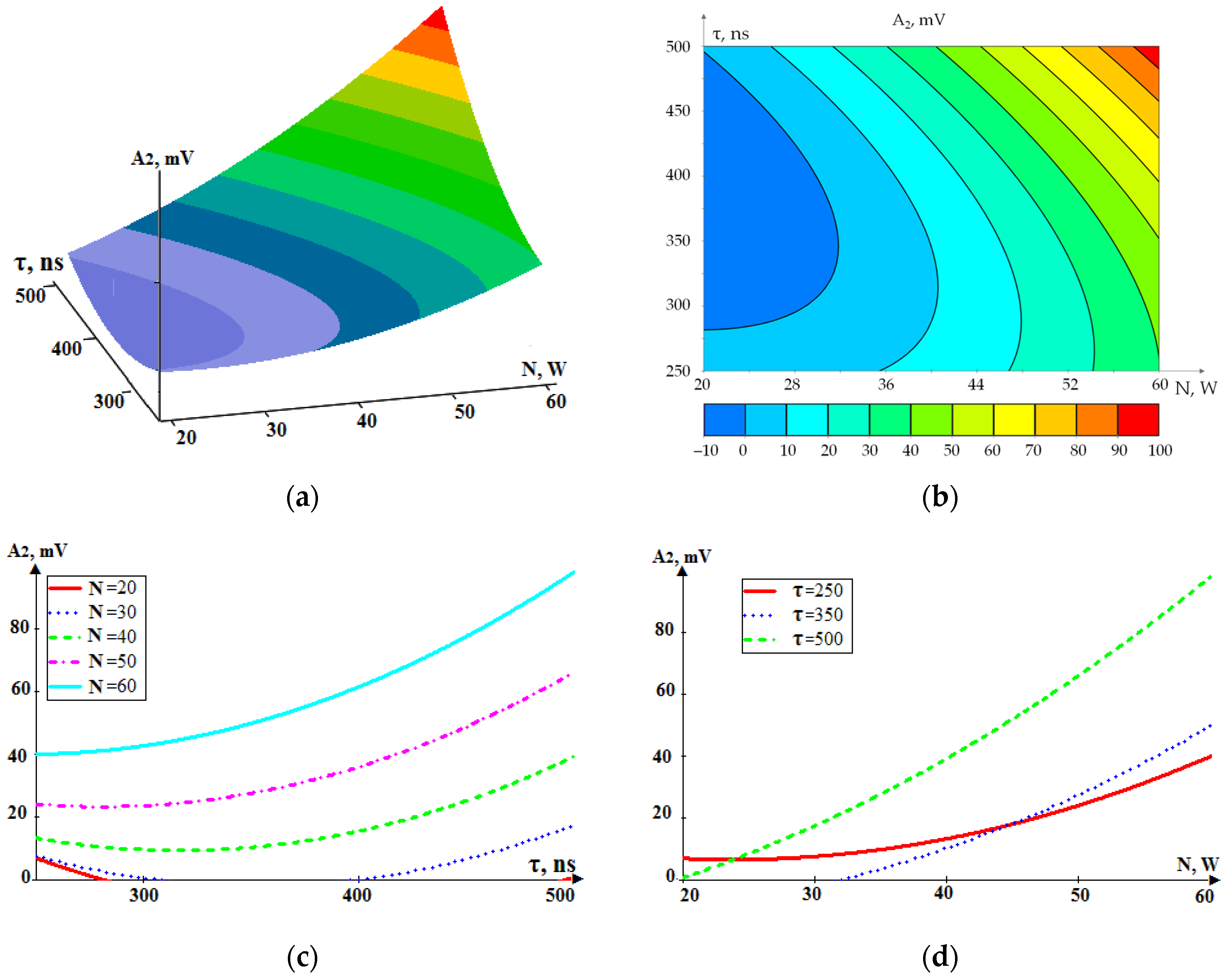
Figure 15.
The dependence of RMS amplitude of the acoustic emission signal in the high-frequency range (32–70 kHz, A2) on the power (N) and pulse duration (τ): (a) general view; (b–d) projections of lines of equal level onto coordinate planes.
Figure 15.
The dependence of RMS amplitude of the acoustic emission signal in the high-frequency range (32–70 kHz, A2) on the power (N) and pulse duration (τ): (a) general view; (b–d) projections of lines of equal level onto coordinate planes.
Figure 16.
The dependence of the volume of removed material Q on the power (N) and pulse duration (τ): (a) general view; (b–d) projections of lines of equal level onto coordinate planes.
Figure 16.
The dependence of the volume of removed material Q on the power (N) and pulse duration (τ): (a) general view; (b–d) projections of lines of equal level onto coordinate planes.
Figure 17.
Joint graphical representation of dependencies of RMS amplitude in low-frequency range A1 (N, τ) and well volume Q (N, τ) converted to percent units (indexed “p”).
Figure 17.
Joint graphical representation of dependencies of RMS amplitude in low-frequency range A1 (N, τ) and well volume Q (N, τ) converted to percent units (indexed “p”).
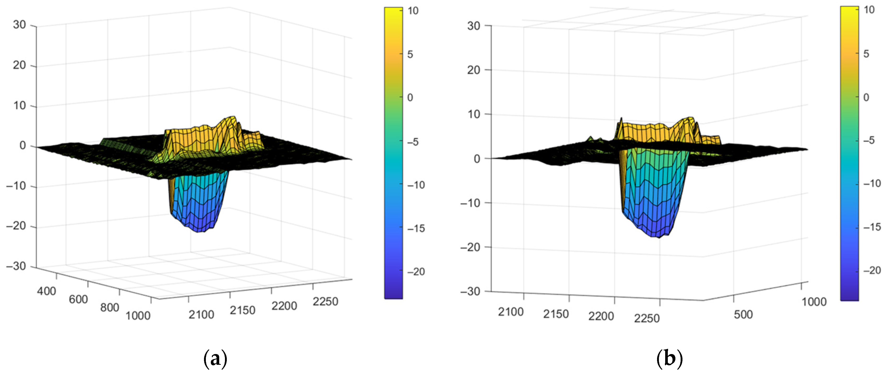
Figure 18.
The distribution of material removed from the well and adhered to the surface of the cutting insert surrounding the well: (a) top view; (b) bottom view.
Figure 18.
The distribution of material removed from the well and adhered to the surface of the cutting insert surrounding the well: (a) top view; (b) bottom view.
Figure 19.
The dependence of the volume of material adhered to the surface surrounding the well, as a percentage of the volume of the well, depending on the power (N) and duration (τ) of laser pulses: (a) general view; (b–d) projections of lines of equal level onto coordinate planes.
Figure 19.
The dependence of the volume of material adhered to the surface surrounding the well, as a percentage of the volume of the well, depending on the power (N) and duration (τ) of laser pulses: (a) general view; (b–d) projections of lines of equal level onto coordinate planes.
Table 1.
The chemical composition of M05 and P10 hard alloys, %.
Table 1.
The chemical composition of M05 and P10 hard alloys, %.
| Hard Alloy | Component, % |
|---|
| WC | TaC | TiC | Co |
|---|
| VK6 (M05) | 92 | 2 | - | 6 |
| T15K6 (P10) | 79 | - | 15 | 6 |
Table 4.
Technical characteristics of the laser unit.
Table 4.
Technical characteristics of the laser unit.
| Characteristic | Description |
|---|
| Laser type | Pulsed fiber laser |
| Operating wavelength, nm | 1064 |
| Maximum power, W | 60 |
| Energy in a radiation pulse, mJ | 2 |
| Pulse duration, ns | From 2 to 500 |
| Software | SHARPLASE SOFTTM based on C++
(version 190627) |
Table 5.
Technical characteristics of the accelerometer.
Table 5.
Technical characteristics of the accelerometer.
| Characteristic | Measuring Unit | Value |
|---|
| Conversion factor | mV/m/s2 | 10 |
| Linear frequency range | Hz | 0.5–15,000 |
| Resonant frequency in axial direction | kHz | >45 |
| Noise level, RMS 1 (1 Hz–10 kHz) | m/s2 | <0.0035 |
Table 6.
Processing modes of the experiment with cutting insert made of T15K6 alloy.
Table 6.
Processing modes of the experiment with cutting insert made of T15K6 alloy.
| Measurement Area | Experiment Number | Processing Mode | Pulse Duration τ, ns | Pulse Power N, W |
| 1 | 1–1 | 1 | 500 | 60 |
| 1–2 | 2 | 50 |
| 1–3 | 3 | 40 |
| 1–4 | 4 | 30 |
| 1–5 | 5 | 20 |
| 2 | 2–1 | 6 | 350 | 60 |
| 2–2 | 7 | 50 |
| 2–3 | 8 | 40 |
| 2–4 | 9 | 30 |
| 2–5 | 10 | 20 |
| 3 | 3–1 | 11 | 250 | 60 |
| 3–2 | 12 | 50 |
| 3–3 | 13 | 40 |
| 3–4 | 14 | 30 |
| 3–5 | 15 | 20 |
Table 2.
The chemical composition of D16 aluminum alloy, %.
Table 2.
The chemical composition of D16 aluminum alloy, %.
| Element | Al | Cu | Mg | Mn | Fe | Si | Zn | Ni | Ti |
|---|
| % | 90.8–94.7 | 3.8–4.9 | 1.2–1.8 | 0.3–0.9 | Up to 0.5 | Up to 0.5 | Up to 0.3 | Up to 0.1 | Up to 0.1 |
Table 3.
The chemical composition of R6M5 high-speed steel, %.
Table 3.
The chemical composition of R6M5 high-speed steel, %.
| Element | Fe | W | Mo | Cr | V | C | Mn | Si | Ni | Co | Cu | P | S |
|---|
| % | From 78.4 | 5.5–6.5 | 4.8–5.3 | 3.8–4.4 | 1.7–2.1 | 0.8–0.9 | 0.2–0.5 | 0.2–0.5 | Up to 0.6 | Up to 0.5 | Up to 0.25 | Up to 0.03 | Up to 0.025 |
Table 7.
Parameters of the formed well profiles.
Table 7.
Parameters of the formed well profiles.
| Number of Pulses | Diameter D, mm | Depth L, mm | Volume of Removed Material Q × 10–5, mm3 |
|---|
| 5 | 0.089 | 0.102 | 35.0 |
| 10 | 0.076 | 0.159 | 72.0 |
| 20 | 0.062 | 0.273 | 83.0 |
| 40 | 0.061 | 0.818 | 86.0 |
| 80 | 0.049 | 1.047 | 89.0 |
Table 8.
Results of the experiment with cutting insert made of T15K6 alloy.
Table 8.
Results of the experiment with cutting insert made of T15K6 alloy.
| Processing Mode | Pulse Duration τ, ns | Pulse Power N, W | RMS Amplitude in 10–28 kHz A1, mV | RMS Amplitude in 32–70 kHz A2, mV | Well Volume Q, µm3 | Ejecta Volume V, % |
|---|
| 1 | 500 | 60 | 166.0 | 100.0 | 25,900.0 | 12.0 |
| 2 | 50 | 110.0 | 70.0 | 20,277.9 | 13.0 |
| 3 | 40 | 60.0 | 35.0 | 12,079.0 | 25.2 |
| 4 | 30 | 22.2 | 13.0 | 5966.0 | 45.7 |
| 5 | 20 | 4.0 | 3.0 | 291.6 | 105.6 |
| 6 | 350 | 60 | 84.7 | 42.4 | 12,999.0 | 22.9 |
| 7 | 50 | 49.7 | 26.2 | 9670.0 | 25.3 |
| 8 | 40 | 22.4 | 12.8 | 4857.0 | 50.2 |
| 9 | 30 | 7.7 | 4.14 | 781.8 | 157.5 |
| 10 | 20 | 0 | 0 | 0 | - |
| 11 | 250 | 60 | 72.4 | 42.0 | 10,819.0 | 7.3 |
| 12 | 50 | 40.1 | 27.5 | 6456.0 | 44.1 |
| 13 | 40 | 15.4 | 12.8 | 3258.0 | 62.8 |
| 14 | 30 | 3.0 | 2.3 | 346.0 | 211.6 |
| 15 | 20 | 0 | 0 | 0 | - |
Table 9.
Function comparison data for RMS amplitude in low-frequency range A1 (N, τ) and well volume Q (N, τ) converted to percent units (p).
Table 9.
Function comparison data for RMS amplitude in low-frequency range A1 (N, τ) and well volume Q (N, τ) converted to percent units (p).
| Functions | Processing Mode |
|---|
| 1 | 2 | 3 | 4 | 5 | 6 | 7 | 8 | 9 | 10 | 11 | 12 | 13 | 14 | 15 |
|---|
| RMS amplitude A1p, % | 100 | 66 | 36 | 13 | 2.4 | 51 | 30 | 13.5 | 4.6 | 0 | 43.6 | 24 | 9.3 | 1.8 | 0 |
| Well volume Qp, % | 100 | 78.3 | 46.6 | 23 | 1.1 | 50.2 | 37.3 | 18.8 | 3 | 0 | 41.8 | 24.9 | 12.6 | 1.3 | 0 |


 ,
, 


