


Deep-Learning-Based Antenna Alignment Prediction for Mobile Indoor Communication
 , , , and
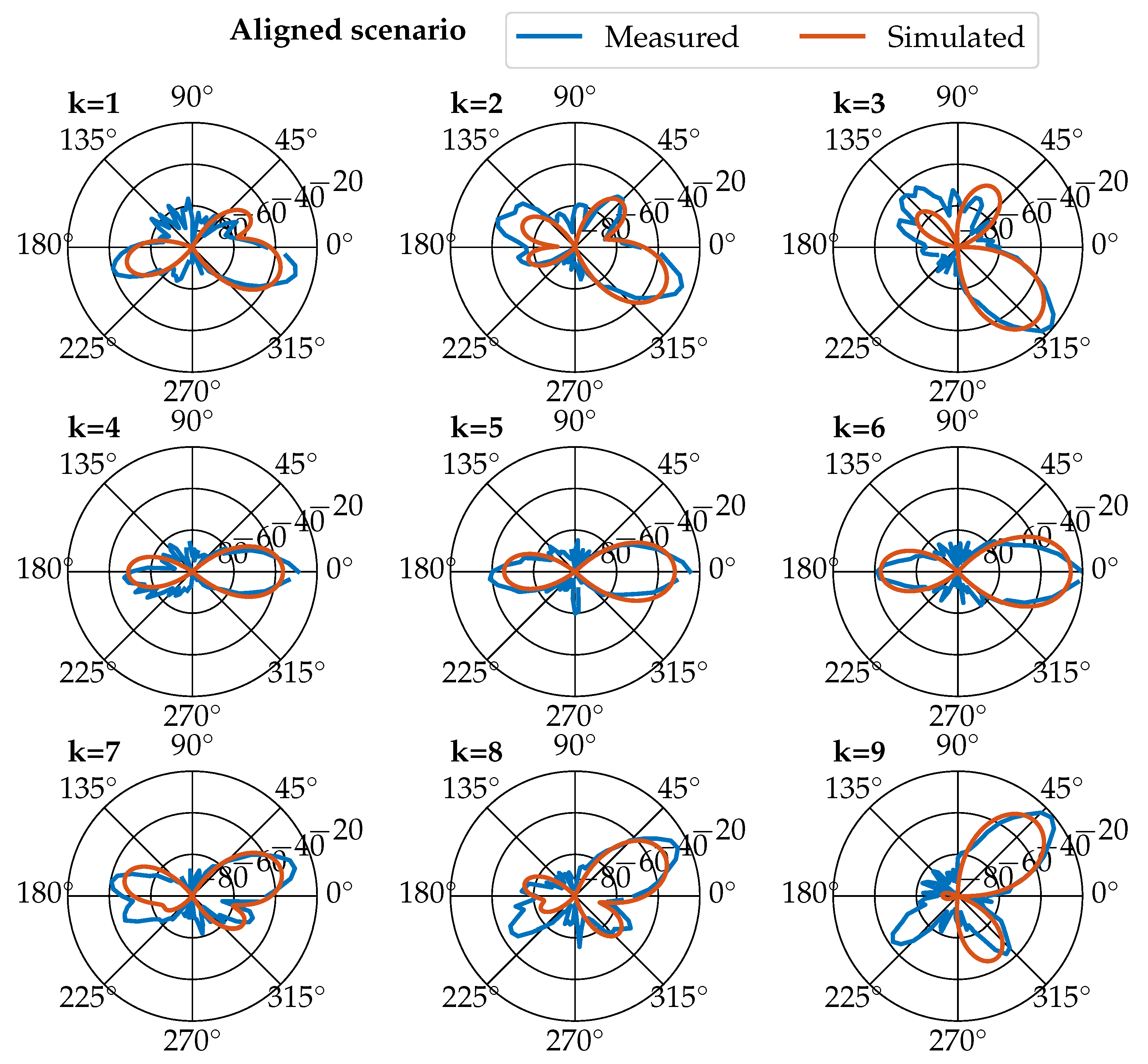
Abstract
1. Introduction
2. Problem Formulation
2.1. Measurement Based Indoor Ray Tracing Simulation
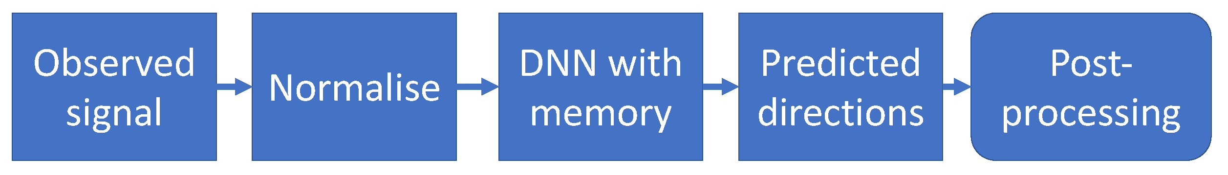
2.2. The Prediction Structure and the Problem to Solve
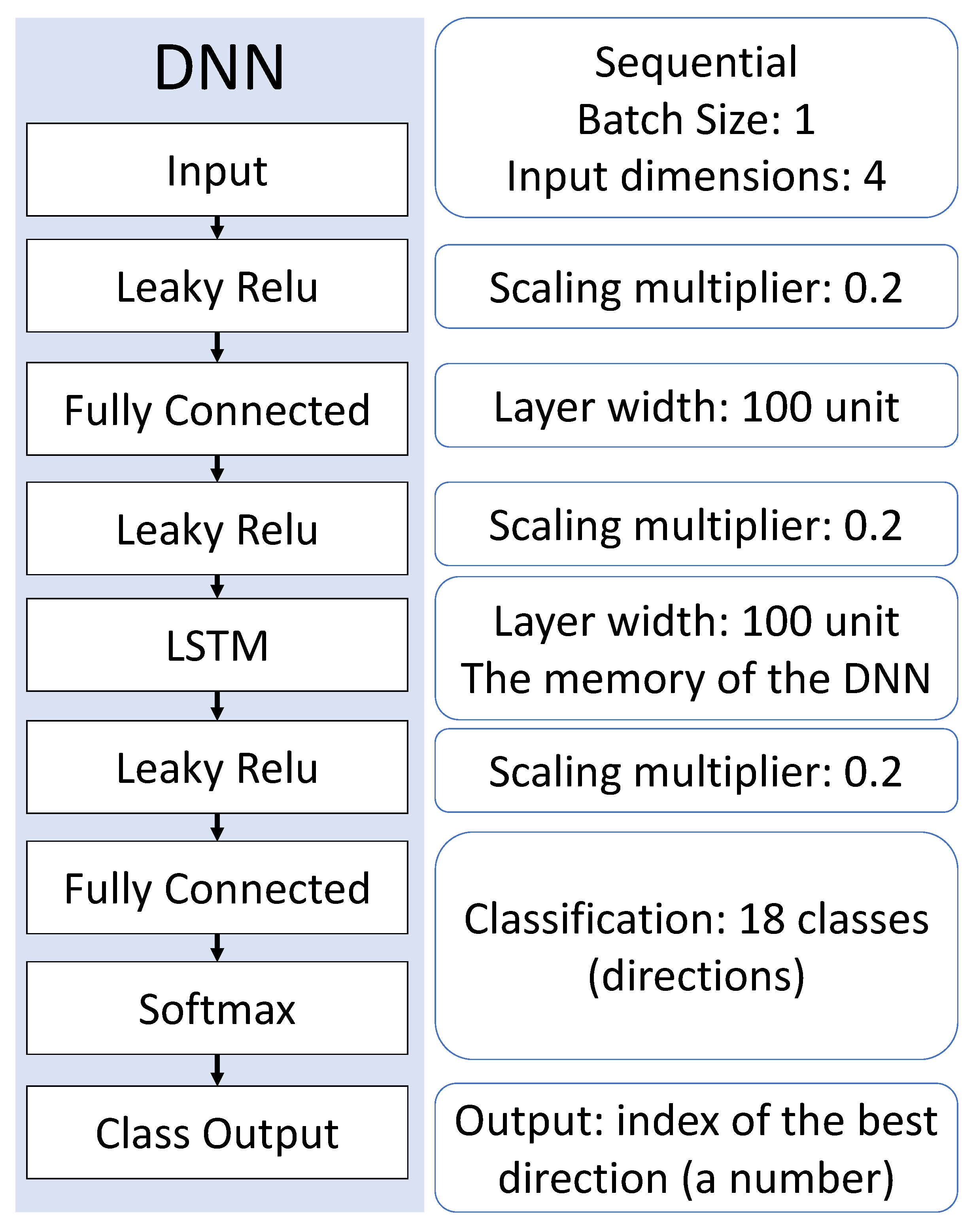
2.3. The Structure of the Used Deep Neural Network
2.4. Main Parameters of the Procedure
- User velocity/sampling frequencies;
- Number of output classes;
- Used received signal directions;
- Used accuracy metric;
- User movement strategy during the training;
- Aligned/unaligned scenario;
- Room structure.
2.4.1. User Velocity and the Sampling Frequencies
2.4.2. Sampling Distance
2.4.3. Number of Output Classes and Used Input Directions
2.4.4. Received Signal Directions and Accuracy Metric
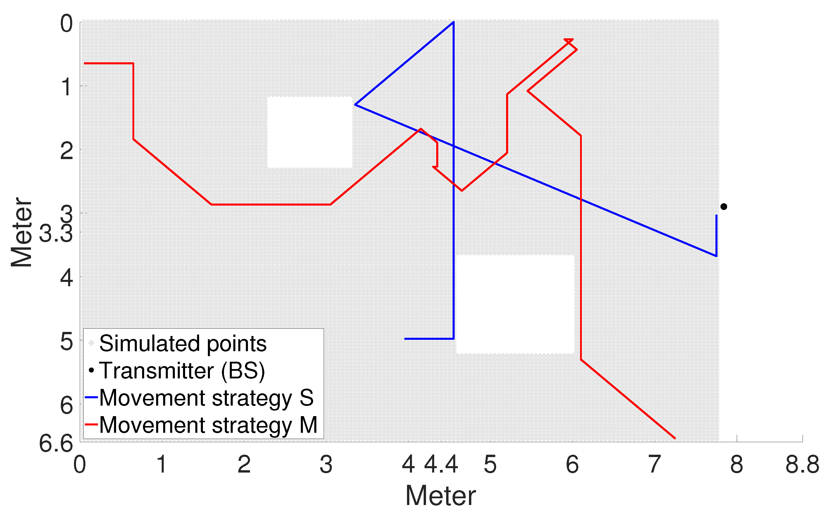
2.4.5. Movement Strategy
- At each point, determine the distance to the nearest impenetrable object.
- A normalised vector is formed from the distances associated with the possible directions of motion (the sum of the vector is 1).
- According to the number of possible step directions, we form normalised vectors, which are the corresponding members of the previous vector and the MBP vector [14].
- From the generated vectors, we form one-to-one Markov chain transition matrices.
- Generating data using matrices: a Markov chain with a matrix of moving user arrivals is used to generate the next arrival point.
2.4.6. Aligned and Unaligned Scenario
2.4.7. The Structure of the Rooms
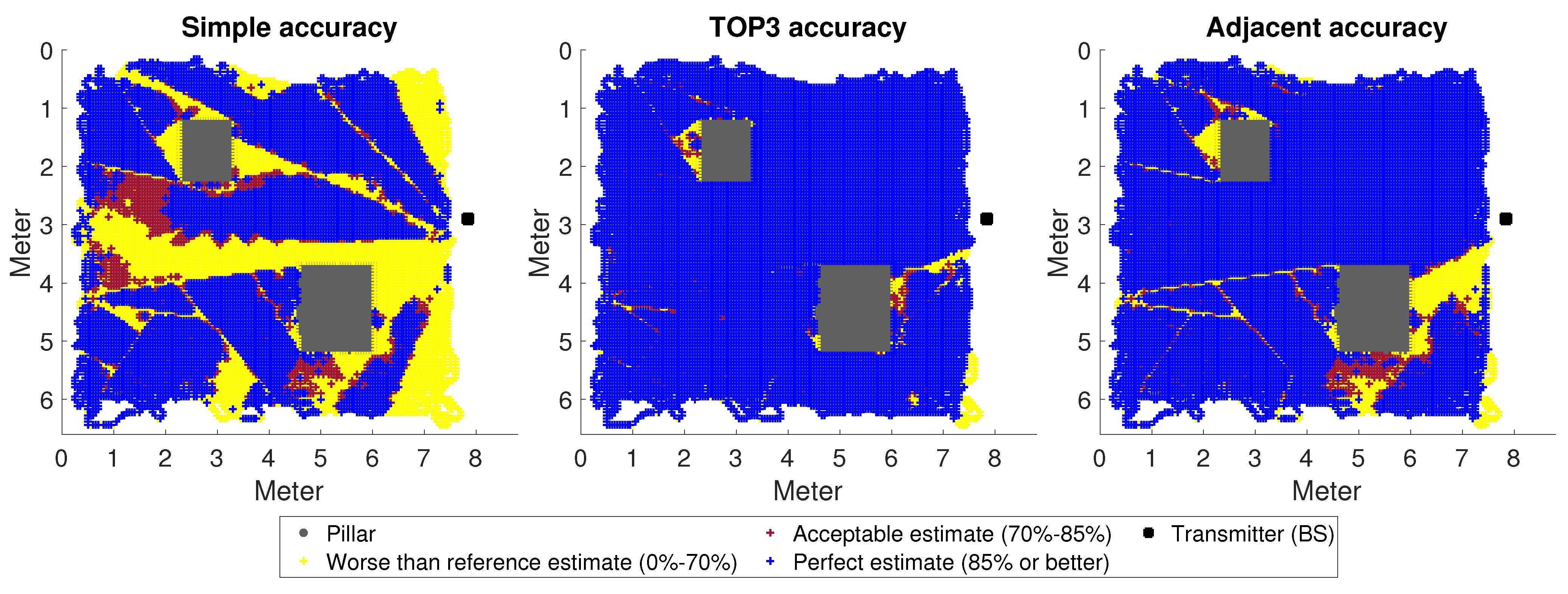
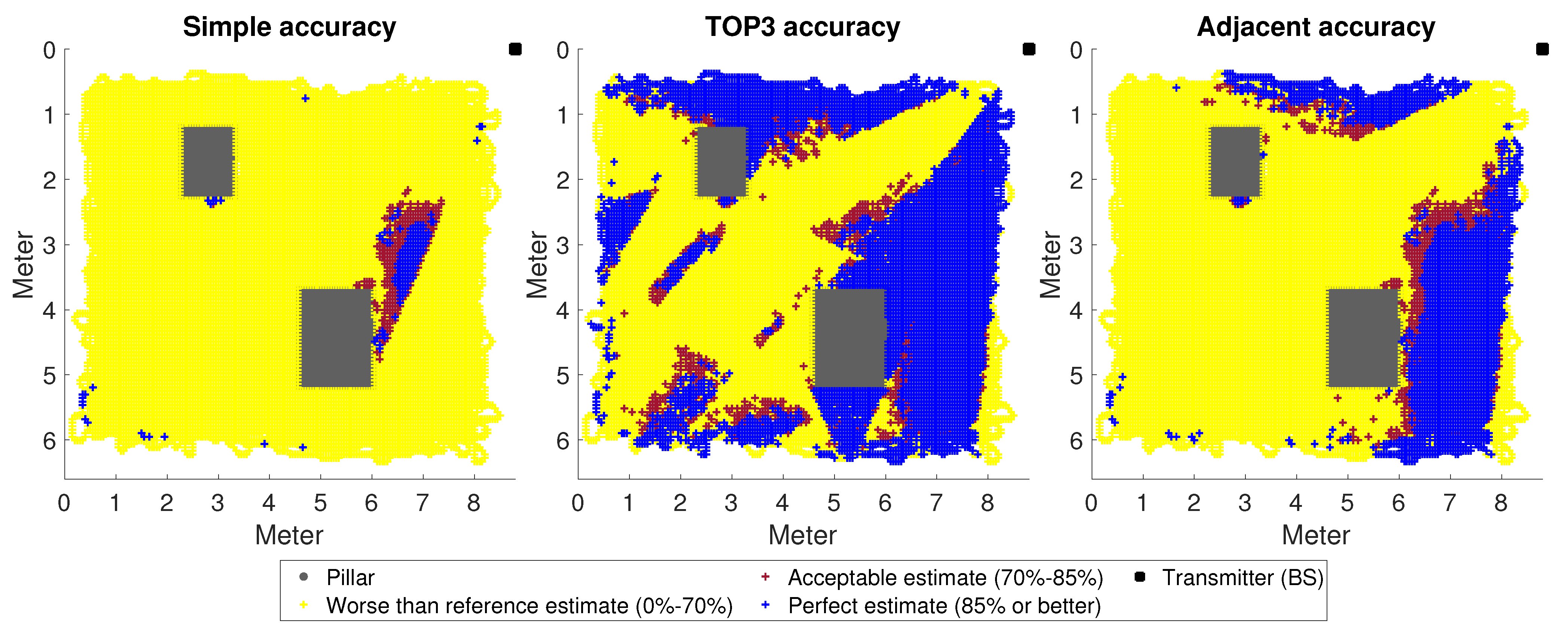
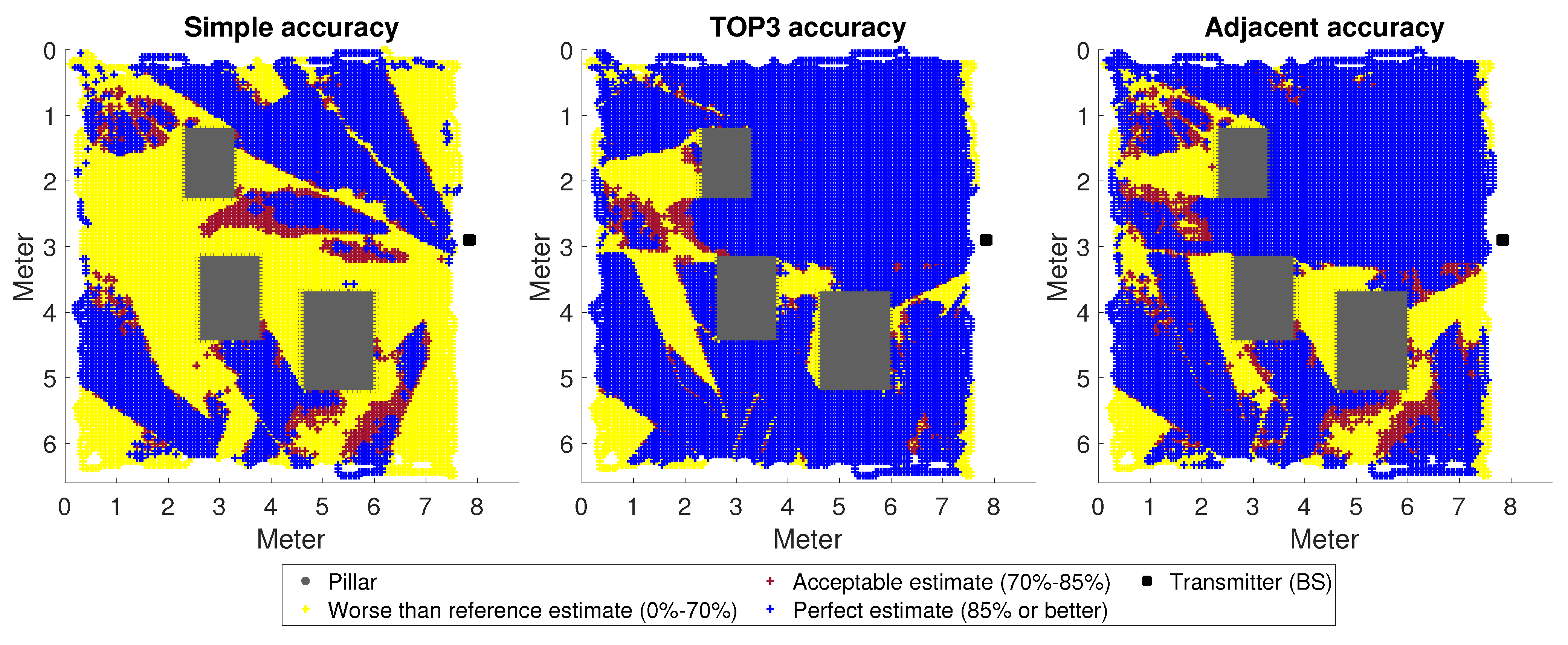
3. Results
The Impact of Changes in the Environment
- Distance between Rooms A1 and A2: 0.63.
- Distance between Rooms A1 and A3: 0.23.
- Distance between Rooms A2 and A3: 0.66.
- Distance between Room A1 and M net training data: 0.23.
- Distance between Room A2 and M net training data: 0.61.
- Distance between Room A3 and M net training data: 0.27.
- Procedures without location information work for this kind of problem.
- Simultaneous UE and BS antenna beamforming can easily become chaotic. Presumably, each mobile device will have at most one antenna/antenna system at a given frequency. Thus, using the presented method, multiple measurements at different positions are required. During this time, the BS should not change its beam position. The synchronisation of this procedure is questionable.
- UE side calculations are resource intensive, simply due to the size of the DNN. It is questionable what the most-efficient implementation might be.
- Applying an online learning process can be also considered, using a net that has already been taught.
- Columns and other impenetrable objects significantly impair accuracy in NLoS cases, especially in unknown rooms. Among other things, this is due to destructive interference at the signal level. However, there are solutions to reduce interference, so the use of such procedures on the UE side is necessary (there is much 5G-related research of this kind, such as [28]).
4. Conclusions and Future Plans
Author Contributions
Funding
Institutional Review Board Statement
Informed Consent Statement
Data Availability Statement
Acknowledgments
Conflicts of Interest
Abbreviations
| AA | Adjacent Accuracy |
| AI | Artificial Intelligence |
| BS | Base Station |
| DNN | Deep Neural Network |
| Leaky Relu | Leaky Rectified linear unit layer |
| LoS | Line-of-Sight |
| LSTM | Long Short-Term Memory |
| MBP | Movement Behaviour Profile |
| ML | Machine Learning |
| mmWave | millimetre Wave |
| NLoS | Non-Line-of-Sight |
| NN | Neural Network |
| RT | Ray Tracing |
| SA | Simple Accuracy |
| TOP3A | TOP3 Accuracy |
| UE | User Equipment |
References
- Bjornson, E.; Van der Perre, L.; Buzzi, S.; Larsson, E.G. Massive MIMO in Sub-6 GHz and mmWave: Physical, Practical, and Use-Case Differences. IEEE Wirel. Commun. 2019, 26, 100–108. [Google Scholar] [CrossRef]
- Zhang, J.; Huang, Y.; Shi, Q.; Wang, J.; Yang, L. Codebook Design for Beam Alignment in Millimeter Wave Communication Systems. IEEE Trans. Commun. 2017, 65, 4980–4995. [Google Scholar] [CrossRef]
- Lin, C.H.; Kao, W.C.; Zhan, S.Q.; Lee, T.S. BsNet: A Deep Learning-Based Beam Selection Method for mmWave Communications. In Proceedings of the 2019 IEEE 90th Vehicular Technology Conference (VTC2019-Fall), Honolulu, HI, USA, 22–25 September 2019; pp. 1–6. [Google Scholar] [CrossRef]
- Kim, Y.; Kim, Y.; Oh, J.; Ji, H.; Yeo, J.; Choi, S.; Ryu, H.; Noh, H.; Kim, T.; Sun, F.; et al. New Radio (NR) and its Evolution toward 5G-Advanced. IEEE Wirel. Commun. 2019, 26, 2–7. [Google Scholar] [CrossRef]
- 3GPP RP-213599; New SI: Study on Artificial Intelligence (AI)/Machine Learning (ML) for NR Air Interface. 3GPP Mobile Competence Centre: Valbonne, France, 2021.
- Gaytare, G.G.; Salau, A.O.; Adame, B.O. Interference mitigation technique for self optimizing Picocell indoor LTE-A networks. Telecommun. Syst. 2022, 81, 549–560. [Google Scholar] [CrossRef]
- Chekole, B.Z.; Olalekan Salau, A.; Kassahun, H.E. Multiband Millimeter Wave Phased Array Antenna Design for 5G Communication. In Proceedings of the 2022 International Conference on Innovation and Intelligence for Informatics, Computing, and Technologies (3ICT), Sakheer, Bahrain, 20–21 November 2022; IEEE: Piscataway, NJ, USA, 2022; pp. 106–111. [Google Scholar] [CrossRef]
- Koutris, A.; Siozos, T.; Kopsinis, Y.; Pikrakis, A.; Merk, T.; Mahlig, M.; Papaharalabos, S.; Karlsson, P. Deep Learning-Based Indoor Localization Using Multi-View BLE Signal. Sensors 2022, 22, 2759. [Google Scholar] [CrossRef] [PubMed]
- Csurgai-Horvath, L.; Horvath, B.; Rieger, I.; Kertesz, J.; Adjei-Frimpong, B. Indoor Propagation Measurements for 5G Networks. In Proceedings of the 2018 11th International Symposium on Communication Systems, Networks & Digital Signal Processing (CSNDSP), Budapest, Hungary, 18–20 July 2018; pp. 1–5. [Google Scholar] [CrossRef]
- Seretis, A.; Sarris, C.D. Toward Physics-Based Generalizable Convolutional Neural Network Models for Indoor Propagation. IEEE Trans. Ant. Prop. 2022, 70, 4112–4126. [Google Scholar] [CrossRef]
- Cisco Visual Networking Index: Forecast and Trends, 2017–2022. Available online: https://twiki.cern.ch/twiki/pub/HEPIX/TechwatchNetwork/HtwNetworkDocuments/white-paper-c11-741490.pdf (accessed on 5 March 2023).
- Moon, S.; Kim, H.; You, Y.H.; Kim, C.H.; Hwang, I. Online learning-based beam and blockage prediction for indoor millimetre-wave communications. ICT Express 2022, 8, 1–6. [Google Scholar] [CrossRef]
- Makara, Á.L.; Csathó, B.T.; Csurgai-Horváth, L.; Horváth, B.P. Measurement-based Indoor Beam Alignment Utilizing Deep Learning. In Proceedings of the 2021 International Conference on Electrical, Computer, Communications and Mechatronics Engineering (ICECCME), Mauritius, Mauritius, 7–8 October 2021; pp. 1–6. [Google Scholar] [CrossRef]
- Makara, Á.L.; Csurgai-Horváth, L. Indoor User Movement Simulation with Markov Chain for Deep Learning Controlled Antenna Beam Alignment. In Proceedings of the 2021 International Conference on Electrical, Computer and Energy Technologies (ICECET), Cape Town, South Africa, 9–10 December 2021; pp. 1–6. [Google Scholar] [CrossRef]
- Ropitault, T.; Blandino, S.; Varshney, N.; Lecci, M.; Testolina, P.; Zorzi, M. A Quasi-Deterministic (Q-D) Channel Implementation in MATLAB Software. 2022. Available online: https://www.nist.gov/services-resources/software/quasi-deterministic-channelrealization-software (accessed on 5 March 2023).
- Zhekov, S.S.; Franek, O.; Pedersen, G.F. Dielectric properties of common building materials for ultrawideband propagation studies. IEEE Ant. Prop. Mag. 2020, 62, 72–81. [Google Scholar] [CrossRef]
- Makara, Á.L.; Csurgai-Horváth, L. Improved Model for Indoor Propagation Loss in the 5G FR2 Frequency Band. Infocommunications J. 2021, 13, 2–10. [Google Scholar] [CrossRef]
- Hagan, M.T.; Demuth, H.B.; Beale, M.H.; De Jésus, O. Neural Network Design, 2nd ed.; Martin T. Hagan: Houston, TX, USA, 2014. [Google Scholar]
- Hochreiter, S.; Schmidhuber, J. Long Short-Term Memory. Neural Comput. 1997, 9, 1735–1780. [Google Scholar] [CrossRef] [PubMed]
- Bishop, C.M. Pattern Recognition and Machine Learning; Information Science and Statistics, Springer: New York, NY, USA, 2006. [Google Scholar]
- Goodfellow, I.; Bengio, Y.; Courville, A. Deep Learning; MIT Press: Cambridge, MA, USA, 2016. [Google Scholar]
- Kingma, D.P.; Ba, J. Adam: A Method for Stochastic Optimization. arXiv 2014, arXiv:1412.6980. [Google Scholar] [CrossRef]
- Koech, K.E. Cross-Entropy Loss Function. 2022. Available online: https://towardsdatascience.com/cross-entropy-loss-function-f38c4ec8643e (accessed on 3 March 2023).
- Murphy, K.P. Machine Learning: A Probabilistic Perspective; Adaptive Computation and Machine Learning Series; MIT Press: Cambridge, MA, USA, 2012. [Google Scholar]
- Maas, A.L.; Hannun, A.Y.; Ng, A.Y. Rectifier nonlinearities improve neural network acoustic models. In ICML Workshop on Deep Learning for Audio, Speech and Language Processing; Computer Science Department, Stanford University: Stanford, CA, USA, 2013. [Google Scholar]
- Makara, Á.L.; Csurgai-Horváth, L. Classification of Indoor Environment in Neural Network Controlled FR2-band Communication. In Proceedings of the 2022 International Conference on Electrical, Computer and Energy Technologies (ICECET), Prague, Czech Republic, 20–22 July 2022; pp. 1–6. [Google Scholar] [CrossRef]
- Tsybakov, A.B. Introduction to Nonparametric Estimation; Springer Series in Statistics; Springer: New York, NY, USA; London, UK, 2009. [Google Scholar]
- Adame, B.O.; Salau, A.O. Genetic Algorithm Based Optimum Finger Selection for Adaptive Minimum Mean Square Error Rake Receivers Discrete Sequence-CDMA Ultra-Wide Band Systems. Wirel. Pers. Commun. 2022, 123, 1537–1551. [Google Scholar] [CrossRef]


Disclaimer/Publisher’s Note: The statements, opinions and data contained in all publications are solely those of the individual author(s) and contributor(s) and not of MDPI and/or the editor(s). MDPI and/or the editor(s) disclaim responsibility for any injury to people or property resulting from any ideas, methods, instructions or products referred to in the content. |
© 2023 by the authors. Licensee MDPI, Basel, Switzerland. This article is an open access article distributed under the terms and conditions of the Creative Commons Attribution (CC BY) license (https://creativecommons.org/licenses/by/4.0/).
Share and Cite
Makara, Á.L.; Csathó, B.T.; Rácz, A.; Borsos, T.; Csurgai-Horváth, L.; Horváth, B.P. Deep-Learning-Based Antenna Alignment Prediction for Mobile Indoor Communication. Sensors 2023, 23, 3375. https://doi.org/10.3390/s23073375
Makara ÁL, Csathó BT, Rácz A, Borsos T, Csurgai-Horváth L, Horváth BP. Deep-Learning-Based Antenna Alignment Prediction for Mobile Indoor Communication. Sensors. 2023; 23(7):3375. https://doi.org/10.3390/s23073375
Chicago/Turabian StyleMakara, Árpád László, Botond Tamás Csathó, András Rácz, Tamás Borsos, László Csurgai-Horváth, and Bálint Péter Horváth. 2023. "Deep-Learning-Based Antenna Alignment Prediction for Mobile Indoor Communication" Sensors 23, no. 7: 3375. https://doi.org/10.3390/s23073375
APA StyleMakara, Á. L., Csathó, B. T., Rácz, A., Borsos, T., Csurgai-Horváth, L., & Horváth, B. P. (2023). Deep-Learning-Based Antenna Alignment Prediction for Mobile Indoor Communication. Sensors, 23(7), 3375. https://doi.org/10.3390/s23073375