
Experimental Investigation of Relative Localization Estimation in a Coordinated Formation Control of Low-Cost Underwater Drones


Abstract
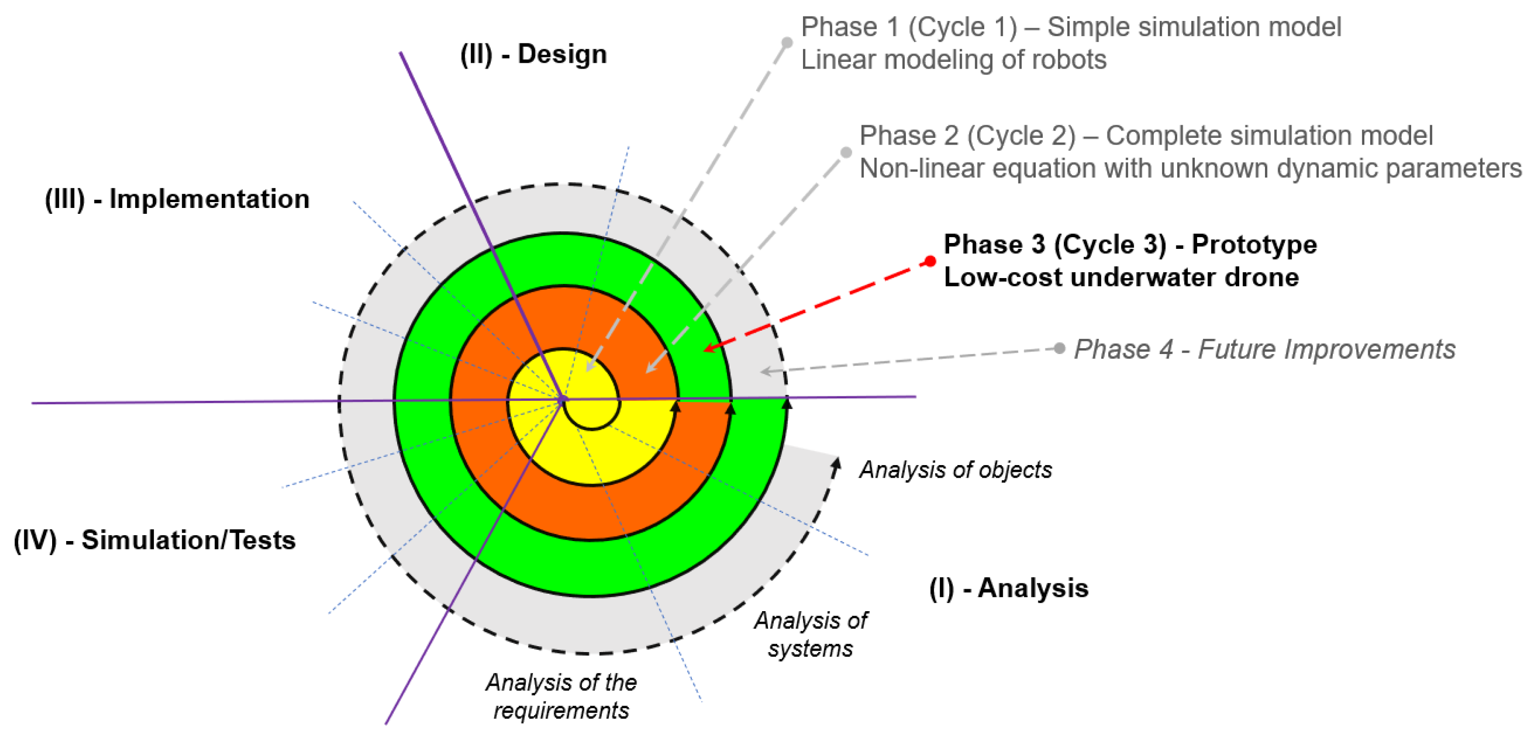
1. Introduction
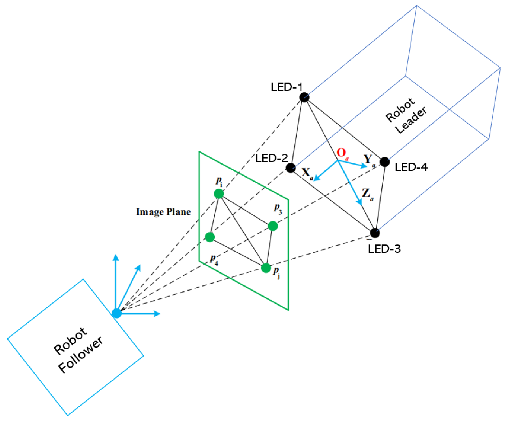
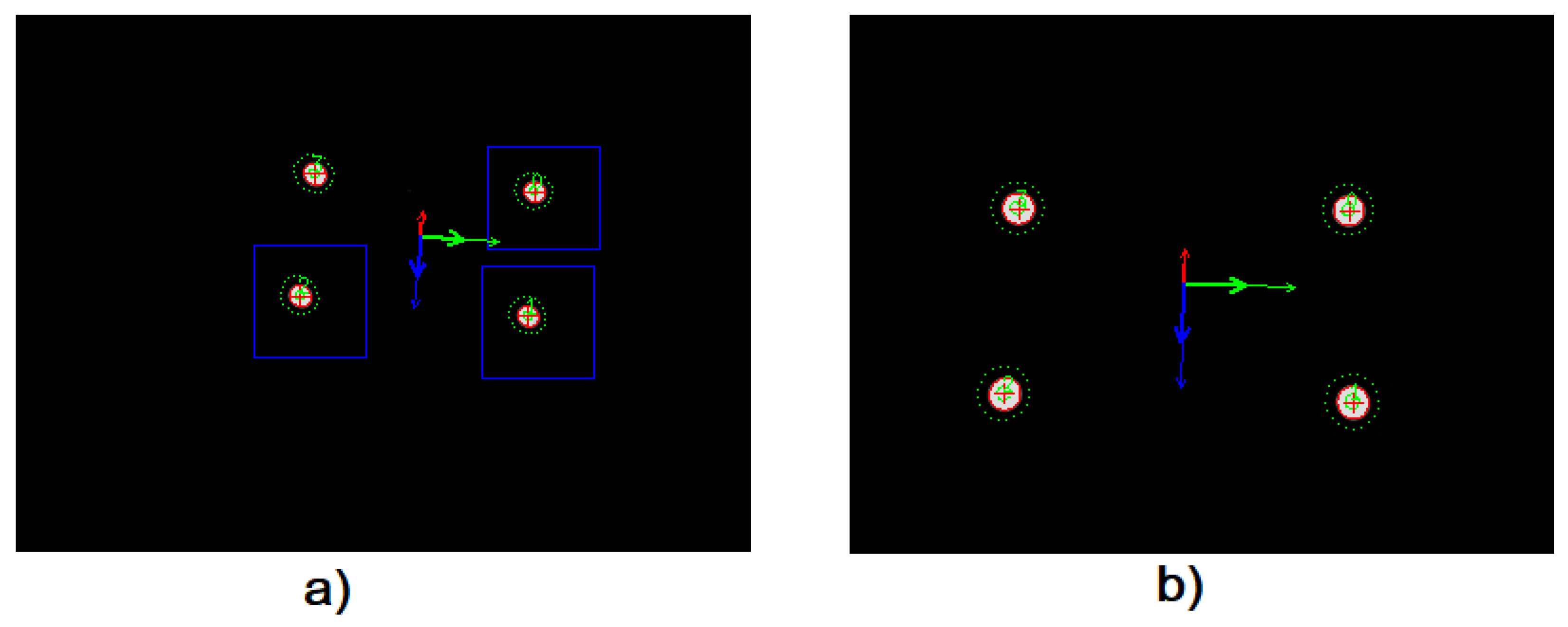
- Proposed an effective prototype using four LEDs for the low-cost underwater drones to be able to determine the relative position between robots and an experimental evaluation of the algorithms for the low-cost underwater drones, which has not yet been investigated to the authors’ knowledge.
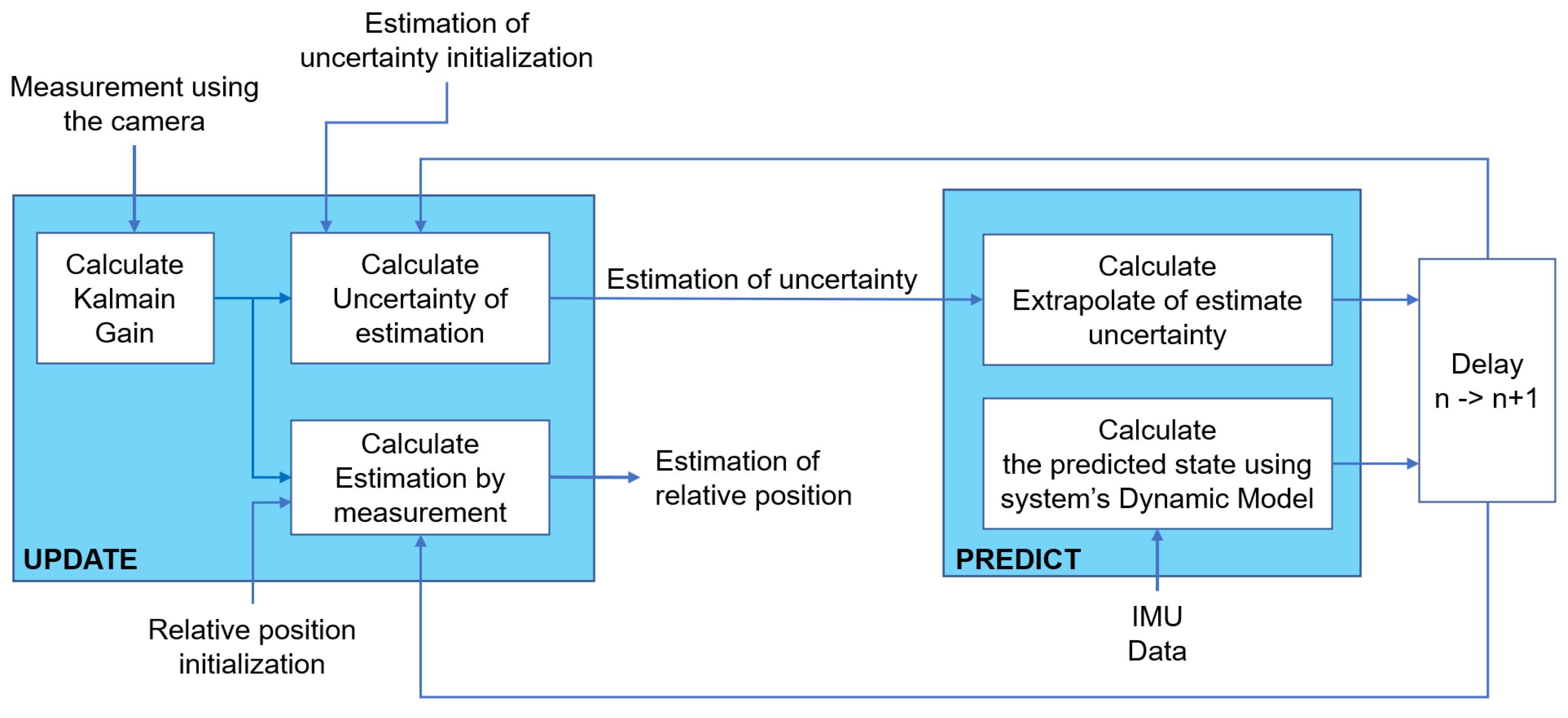
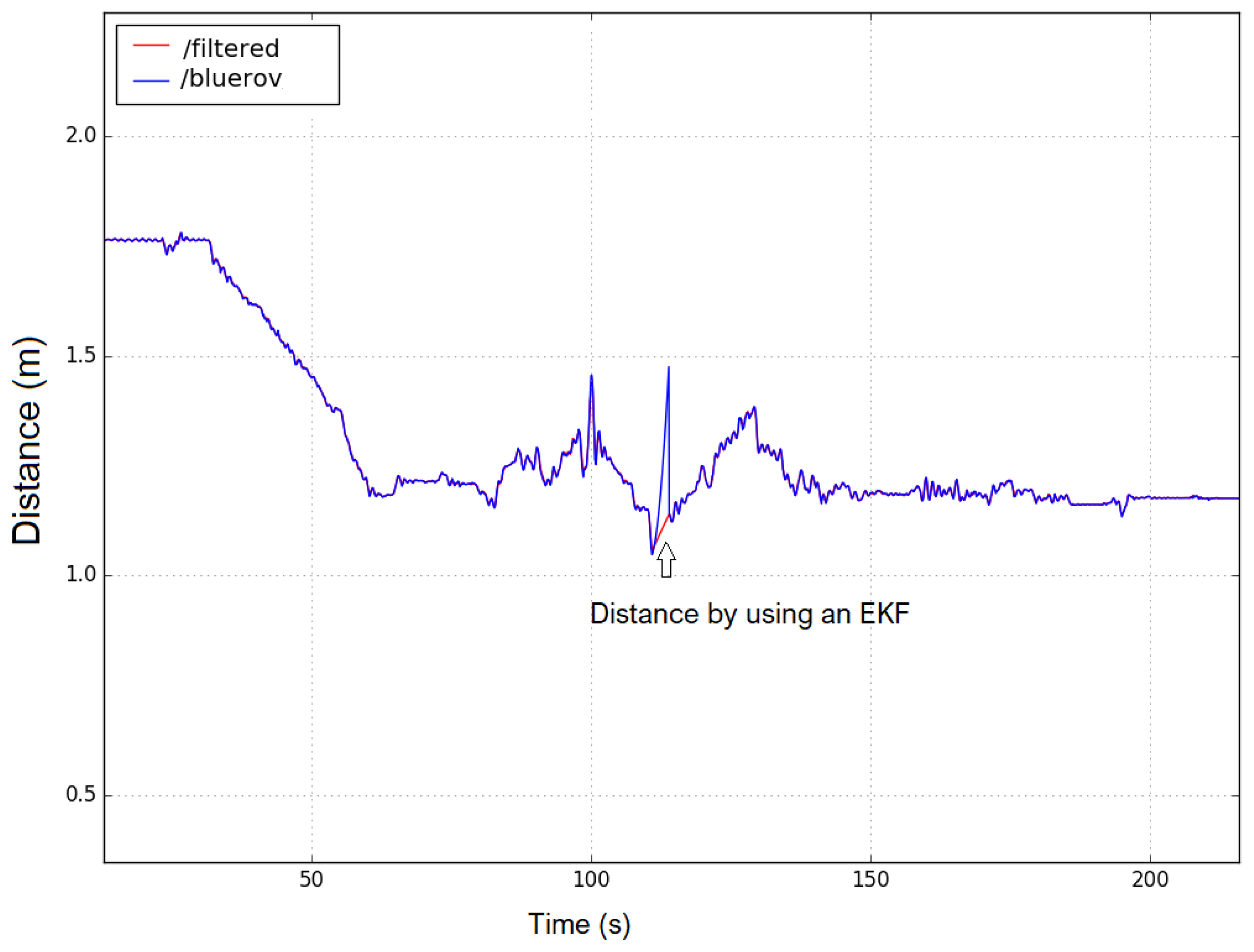
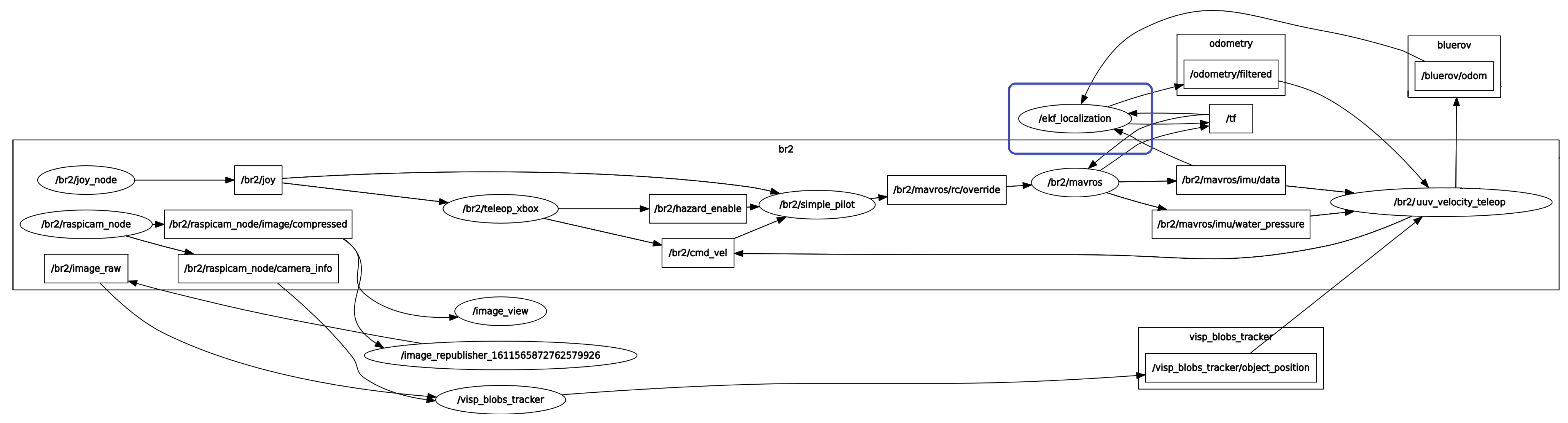
- Proposed to use an EKF to estimate the position of the underwater vehicle follower-leader in case the robot is out of view of the camera. Compared with [30], the dynamic adaptive Kalman filter was used to navigate a group of AUVs in cases with and without GNSS. We implemented EKF for underwater vehicles and used only vision and IMU data. The use of cameras is low cost compared to positioning methods using sonar technology, which according to article [15], costs thousands to hundreds of thousands of dollars.
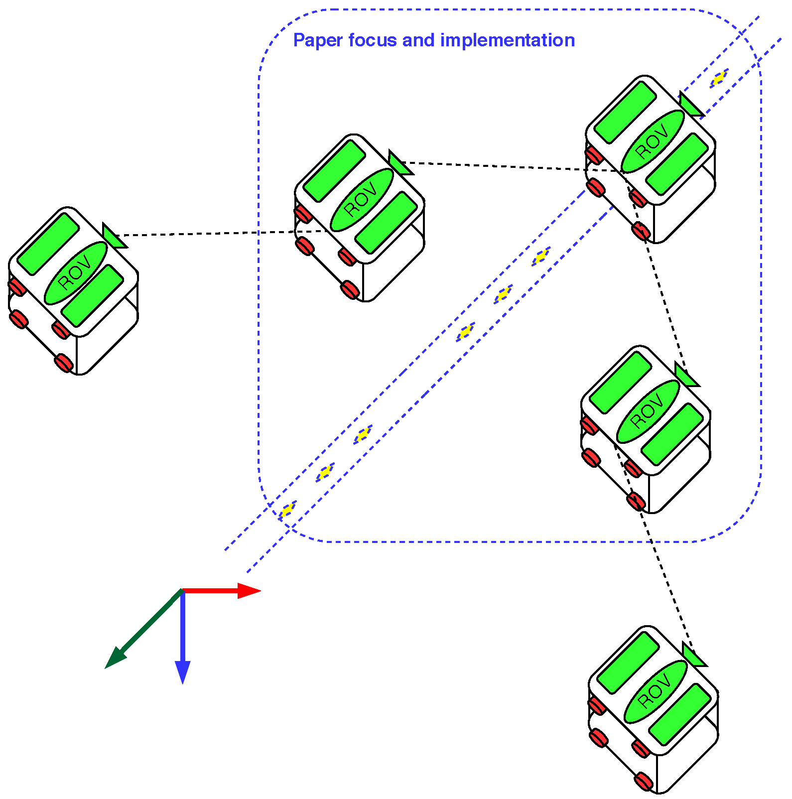
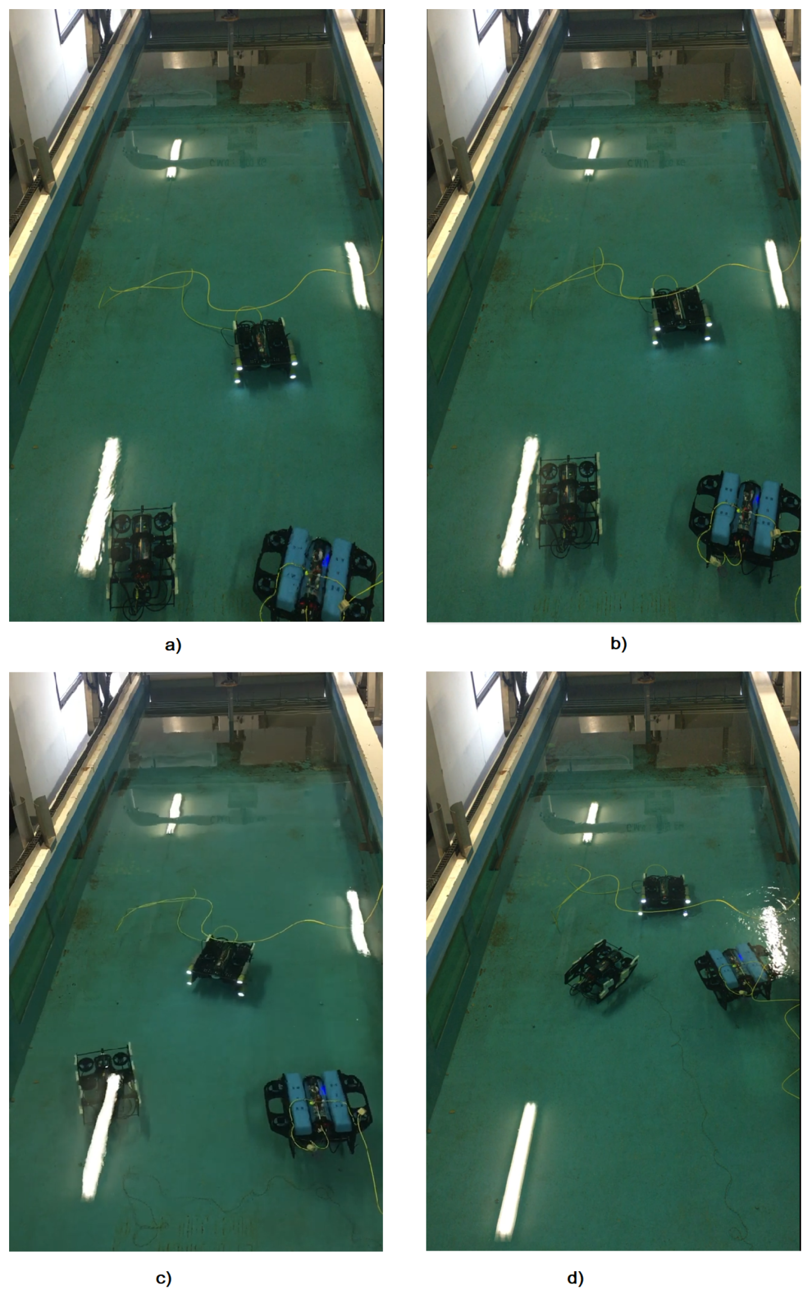
- Tested coordination control algorithms (i.e., formation control) in real environment conditions.
2. Related Work
2.1. Low-Cost Underwater Drone Modeling
2.2. Formation Tracking Control
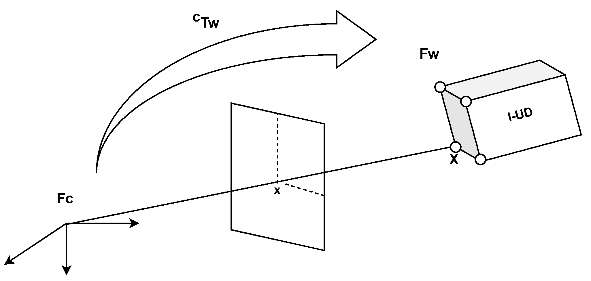
2.3. Vision-Based Pose Estimation
2.4. Theory of Extended KALMAN Filter
3. Implement Relative Positioning for l-UD Followers
4. Experiment Setup
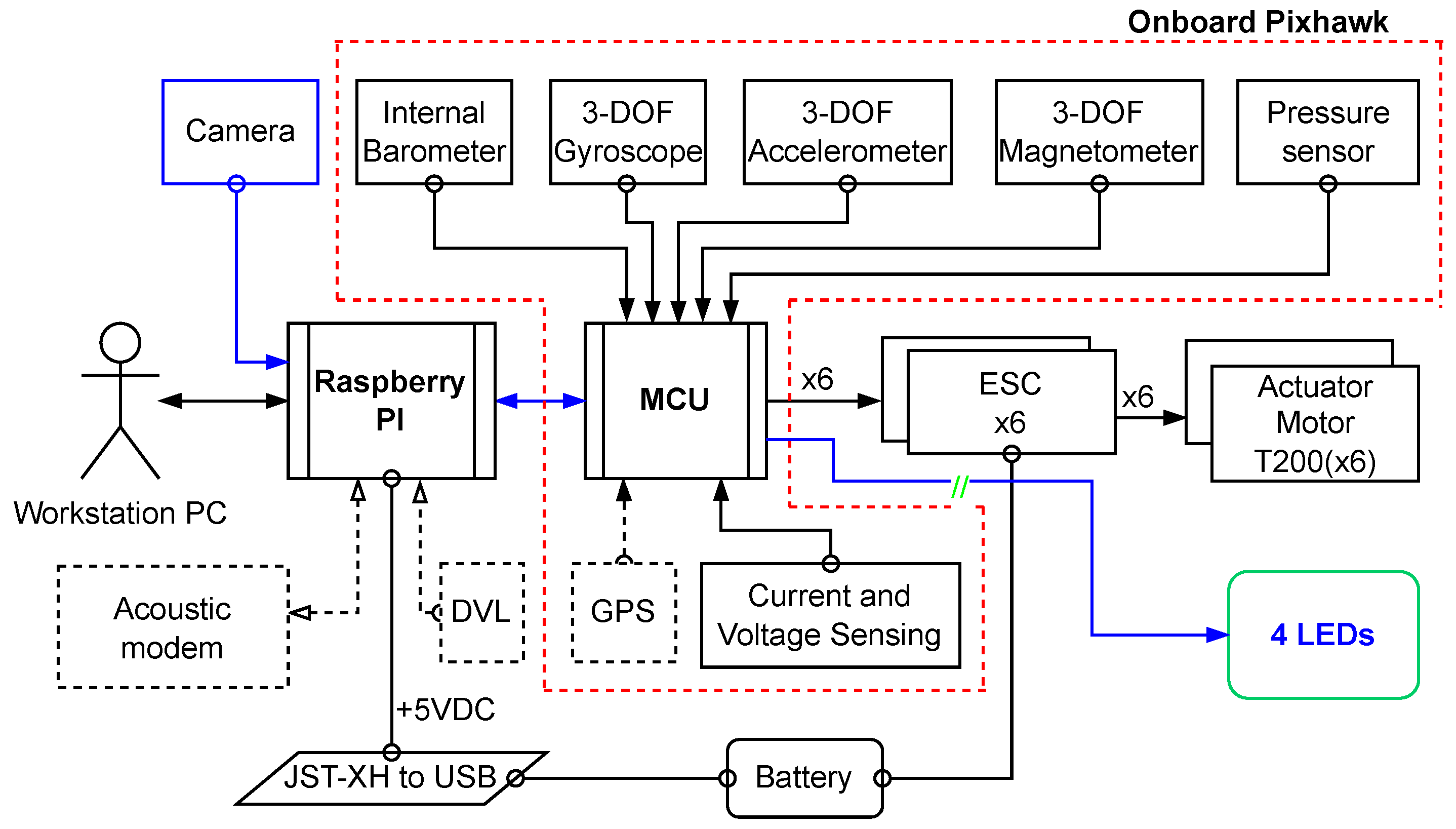
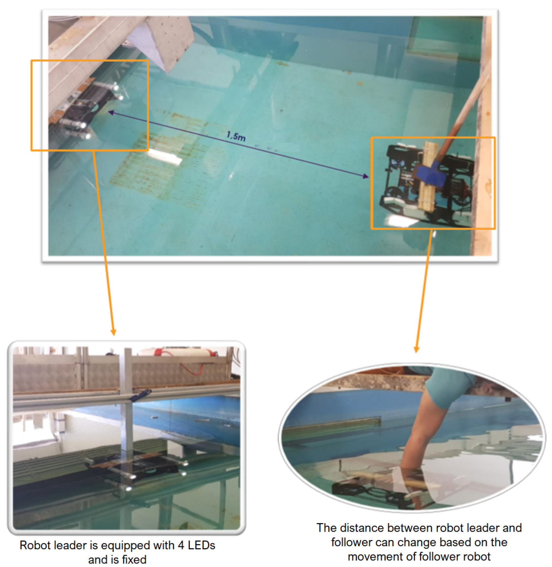
4.1. Low-Cost Underwater Drone BlueROV with LED
4.2. Determination of the Function of the Real Distance and the Distance Measured by the Camera
4.3. The Experiment with Three Robots
5. Conclusions
Author Contributions
Funding
Institutional Review Board Statement
Informed Consent Statement
Data Availability Statement
Conflicts of Interest
Abbreviations
| AUV | Autonomous underwater vehicle |
| EKF | Extended Kalman filter |
| FOV | Field of view |
| IMU | Inertial measurement unit |
| LED | Light-emitting diode |
| l-UD | Low-cost underwater drone |
| PD | Proportional derivative |
| ROV | Remotely operated vehicle |
| UAV | Unmanned aerial vehicle |
| UGV | Unmanned ground vehicles |
| UUV | Unmanned underwater vehicles |
| PWM | Pulse-width modulation |
| USBL | Ultra-short baseline |
| GNSS | Global navigation satellite systems |
Appendix A

References
- Qin, J.; Gao, H.; Zheng, W.X. Second-order consensus for multi-agent systems with switching topology and communication delay. Syst. Control. Lett. 2011, 60, 390–397. [Google Scholar] [CrossRef]
- Qin, J.; Yu, C.; Gao, H. Coordination for Linear Multiagent Systems With Dynamic Interaction Topology in the Leader-Following Framework. IEEE Trans. Ind. Electron. 2014, 61, 2412–2422. [Google Scholar] [CrossRef]
- Qin, J.; Gao, H. A Sufficient Condition for Convergence of Sampled-Data Consensus for Double-Integrator Dynamics with Nonuniform and Time-Varying Communication Delays. IEEE Trans. Autom. Control 2012, 57, 2417–2422. [Google Scholar] [CrossRef]
- Xiao, F.; Wang, L. Asynchronous Consensus in Continuous-Time Multi-Agent Systems With Switching Topology and Time-Varying Delays. IEEE Trans. Autom. Control 2008, 53, 1804–1816. [Google Scholar] [CrossRef]
- Li, H.; Shi, Y. Robust Receding Horizon Control for Networked and Distributed Nonlinear Systems; Springer: Cham, Switzerland, 2017. [Google Scholar] [CrossRef]
- Shi, G.; Johansson, K.H. Randomized optimal consensus of multi-agent systems. Automatica 2012, 48, 3018–3030. [Google Scholar] [CrossRef]
- Yu, W.; DeLellis, P.; Chen, G.; di Bernardo, M.; Kurths, J. Distributed Adaptive Control of Synchronization in Complex Networks. IEEE Trans. Autom. Control 2012, 57, 2153–2158. [Google Scholar] [CrossRef]
- Qin, J.; Zheng, W.X.; Gao, H. Coordination of Multiple Agents With Double-Integrator Dynamics Under Generalized Interaction Topologies. IEEE Trans. Syst. Man Cybern. Part B Cybern. 2012, 42, 44–57. [Google Scholar] [CrossRef]
- Qin, J.; Gao, H.; Zheng, W.X. Exponential Synchronization of Complex Networks of Linear Systems and Nonlinear Oscillators: A Unified Analysis. IEEE Trans. Neural Netw. Learn. Syst. 2015, 26, 510–521. [Google Scholar] [CrossRef]
- Yang, T.; Roy, S.; Wan, Y.; Saberi, A. Constructing consensus controllers for networks with identical general linear agents. Int. J. Robust Nonlinear Control 2011, 21, 1237–1256. [Google Scholar] [CrossRef]
- Peng, Z.; Wang, D.; Shi, Y.; Wang, H.; Wang, W. Containment control of networked autonomous underwater vehicles with model uncertainty and ocean disturbances guided by multiple leaders. Inf. Sci. 2015, 316, 163–179. [Google Scholar] [CrossRef]
- Qin, J.; Ma, Q.; Shi, Y.; Wang, L. Recent Advances in Consensus of Multi-Agent Systems: A Brief Survey. IEEE Trans. Ind. Electron. 2017, 64, 4972–4983. [Google Scholar] [CrossRef]
- Cao, Y.; Yu, W.; Ren, W.; Chen, G. An Overview of Recent Progress in the Study of Distributed Multi-Agent Coordination. IEEE Trans. Ind. Informatics 2013, 9, 427–438. [Google Scholar] [CrossRef]
- Pham, H.A.; Soriano, T.; Ngo, V.H.; Gies, V. Distributed Adaptive Neural Network Control Applied to a Formation Tracking of a Group of Low-Cost Underwater Drones in Hazardous Environments. Appl. Sci. 2020, 10, 1732. [Google Scholar] [CrossRef]
- Paull, L.; Saeedi, S.; Seto, M.; Li, H. AUV Navigation and Localization: A Review. IEEE J. Ocean. Eng. 2014, 39, 131–149. [Google Scholar] [CrossRef]
- Chen, S.; Yin, D.; Niu, Y. A Survey of Robot Swarms’ Relative Localization Method. Sensors 2022, 22, 4424. [Google Scholar] [CrossRef]
- Garcia, J.G.; Gomez-Espinosa, A.; Cuan-Urquizo, E.; Valdovinos, L.G.G.; Salgado-Jimenez, T.; Cabello, J.A.E. Autonomous Underwater Vehicles: Localization, Navigation, and Communication for Collaborative Missions. Appl. Sci. 2020, 10, 1256. [Google Scholar] [CrossRef]
- Alatise, M.; Hancke, G. Pose Estimation of a Mobile Robot Based on Fusion of IMU Data and Vision Data Using an Extended Kalman Filter. Sensors 2017, 17, 2164. [Google Scholar] [CrossRef]
- Bosch, J.; Gracias, N.; Ridao, P.; Istenic, K.; Ribas, D. Close-Range Tracking of Underwater Vehicles Using Light Beacons. Sensors 2016, 16, 429. [Google Scholar] [CrossRef]
- Cao, Z.; Liu, R.; Yuen, C.; Athukorala, A.; Ng, B.K.K.; Mathanraj, M.; Tan, U.X. Relative Localization of Mobile Robots with Multiple Ultra-WideBand Ranging Measurements. arXiv 2017. [Google Scholar] [CrossRef]
- Bosse, M.; Zlot, R. Map Matching and Data Association for Large-Scale Two-dimensional Laser Scan-based SLAM. Int. J. Robot. Res. 2008, 27, 667–691. [Google Scholar] [CrossRef]
- Durrant-Whyte, H.; Bailey, T. Simultaneous localization and mapping: Part I. IEEE Robot. Autom. Mag. 2006, 13, 99–110. [Google Scholar] [CrossRef]
- Montemerlo, M.; Thrun, S.; Koller, D.; Wegbreit, B. FastSLAM: A Factored Solution to the Simultaneous Localization and Mapping Problem. In Proceedings of the Eighteenth National Conference on Artificial Intelligence, Edmonton, Alberta, Canada, 28 July 2002; American Association for Artificial Intelligence: Palo Alto, CA, USA, 2002; pp. 593–598. [Google Scholar]
- Thrun, S.; Montemerlo, M. The Graph SLAM Algorithm with Applications to Large-Scale Mapping of Urban Structures. Int. J. Robot. Res. 2006, 25, 403–429. [Google Scholar] [CrossRef]
- Allibert, G.; Hua, M.D.; Krupínski, S.; Hamel, T. Pipeline following by visual servoing for Autonomous Underwater Vehicles. Control Eng. Pract. 2019, 82, 151–160. [Google Scholar] [CrossRef]
- Shkurti, F.; Chang, W.D.; Henderson, P.; Islam, M.J.; Higuera, J.C.G.; Li, J.; Manderson, T.; Xu, A.; Dudek, G.; Sattar, J. Underwater Multi-Robot Convoying using Visual Tracking by Detection. In Proceedings of the 2017 IEEE/RSJ International Conference on Intelligent Robots and Systems (IROS), Vancouver, BC, Canada, 24–28 September 2017. [Google Scholar]
- Manderson, T.; Higuera, J.C.G.; Cheng, R.; Dudek, G. Vision-based Autonomous Underwater Swimming in Dense Coral for Combined Collision Avoidance and Target Selection. In Proceedings of the IEEE/RSJ International Conference on Intelligent Robots and Systems (IROS), Madrid, Spain, 1–5 October 2018. [Google Scholar]
- Abreu, P.C.; Pascoal, A.M. Formation Control in the scope of the MORPH project. Part I: Theoretical Foundations. IFAC-PapersOnLine 2015, 48, 244–249. [Google Scholar] [CrossRef]
- Abreu, P.C.; Bayat, M.; Pascoal, A.M.; Botelho, J.; Góis, P.; Ribeiro, J.; Ribeiro, M.; Rufino, M.; Sebastião, L.; Silva, H. Formation Control in the scope of the MORPH project. Part II: Implementation and Results. IFAC-PapersOnLine 2015, 48, 250–255. [Google Scholar] [CrossRef]
- Zhang, J.; Zhou, W.; Wang, X. UAV Swarm Navigation Using Dynamic Adaptive Kalman Filter and Network Navigation. Sensors 2021, 21, 5374. [Google Scholar] [CrossRef] [PubMed]
- Peng, Z.; Wang, D.; Chen, Z.; Hu, X.; Lan, W. Adaptive Dynamic Surface Control for Formations of Autonomous Surface Vehicles With Uncertain Dynamics. IEEE Trans. Control Syst. Technol. 2013, 21, 513–520. [Google Scholar] [CrossRef]
- Pham, H.A. Coordination de Systèmes Sous-Marins Autonomes Basée sur une Méthodologie Intégrée dans un Environnement Open-Source. Ph.D. Thesis, University of Toulon, La Valette-du-Var, France, 2021. [Google Scholar]
- Marchand, E.; Uchiyama, H.; Spindler, F. Pose estimation for augmented reality and a hands-on survey. IEEE Trans. Vis. Comput. Graph. 2016, 22, 2633–2651. [Google Scholar] [CrossRef]
- Wang, P.; Xu, G.; Cheng, Y.; Yu, Q. A simple, robust and fast method for the perspective-n-point Problem. Pattern Recognit. Lett. 2018, 108, 31–37. [Google Scholar] [CrossRef]
- Comport, A.I.; Marchand, E.; Pressigout, M.; Chaumette, F. Real-Time Markerless Tracking for AugmentedReality: The Virtual Visual Servoing Framework. IEEE Trans. Vis. Comput. Graph. 2006, 12, 615–628. [Google Scholar] [CrossRef]
- BlueRobotics. BlueROV2 Assembly; BlueRobotics: Torrance, CA, USA, 2016. [Google Scholar]
- Moore, T.; Stouch, D. A Generalized Extended Kalman Filter Implementation for the Robot Operating System. In Proceedings of the 13th International Conference on Intelligent Autonomous Systems (IAS-13), Padova, Italy, 15–18 July 2014. [Google Scholar]


| Notation | Name | Dimensions |
|---|---|---|
| State vector | ||
| Output vector | ||
| F | State transition matrix | |
| Input variable | ||
| G | Matrix control | |
| P | Estimation of uncertainty | |
| Q | Uncertainty on process noise | |
| R | Uncertainty of measurements | |
| Process noise vector | ||
| Measurement noise vector | ||
| H | Observation matrix | |
| K | Kalman gain | |
| n | Discrete time index | – |
Disclaimer/Publisher’s Note: The statements, opinions and data contained in all publications are solely those of the individual author(s) and contributor(s) and not of MDPI and/or the editor(s). MDPI and/or the editor(s) disclaim responsibility for any injury to people or property resulting from any ideas, methods, instructions or products referred to in the content. |
© 2023 by the authors. Licensee MDPI, Basel, Switzerland. This article is an open access article distributed under the terms and conditions of the Creative Commons Attribution (CC BY) license (https://creativecommons.org/licenses/by/4.0/).
Share and Cite
Soriano, T.; Pham, H.A.; Gies, V. Experimental Investigation of Relative Localization Estimation in a Coordinated Formation Control of Low-Cost Underwater Drones. Sensors 2023, 23, 3028. https://doi.org/10.3390/s23063028
Soriano T, Pham HA, Gies V. Experimental Investigation of Relative Localization Estimation in a Coordinated Formation Control of Low-Cost Underwater Drones. Sensors. 2023; 23(6):3028. https://doi.org/10.3390/s23063028
Chicago/Turabian StyleSoriano, Thierry, Hoang Anh Pham, and Valentin Gies. 2023. "Experimental Investigation of Relative Localization Estimation in a Coordinated Formation Control of Low-Cost Underwater Drones" Sensors 23, no. 6: 3028. https://doi.org/10.3390/s23063028
APA StyleSoriano, T., Pham, H. A., & Gies, V. (2023). Experimental Investigation of Relative Localization Estimation in a Coordinated Formation Control of Low-Cost Underwater Drones. Sensors, 23(6), 3028. https://doi.org/10.3390/s23063028