

A Robust Automated Analog Circuits Classification Involving a Graph Neural Network and a Novel Data Augmentation Strategy

 ,
, 
 ,
,  and
and 
Abstract
1. Introduction
- Assess the importance of analog circuits’ classification in different relevant application areas.
- A critical comprehensive review of the related current state-of-the-art. Besides a literature review, we also formulate a comprehensive ontology, starting from the netlists, for transforming a given analog circuit unto a corresponding graph model, and, further, a modeling work-flow of using machine methods (here graph neural networks) for solving the task of analog circuits’ classification or recognition.
- Suggest a Graph Convolutional Network (GCN) model for analog circuit classification: we develop and fine-tune a Graph Convolutional Network (GCN) architecture that may be used for structure identification in general, but here we spot the light on a “graph classification” endeavor.
- Suggest a novel augmentation strategy (in face of eventually limited training dataset(s) in practical settings): we develop and validate some innovative dataset augmentation concepts, which have a positive and significant boosting effect on the performance of the suggested GCN-based graph classifier model.
- To better underscore the novelty of the concept developed, a conceptual and qualitative comparison is performed between the concept and results of this paper and a selection of most recent competing concepts from the very recent related works.
2. Importance and Comprehensive Formulation of Core Requirements for a Robust Classification of Analog Circuits Module
- Consider circuit topology selection. Traditionally, the selection is made manually based on the experts’ deep knowledge of circuit design, while automating the topology for the purposes of addressing both power consumption and functionality in the face of different possible topologies from different technologies. Indeed, analog circuits classification support an automated topology selection in that it gives the knowledge needed to either select proper topologies or tune specific topology selection optimization processes [8,9,10].
- Consider sizing rules or the sizing process of analog circuits. It is well known that the sizing of analog circuit elements or blocks is one of the biggest challenges for designers, as circuits’ performance highly depends on the primitives’ dimensions [3]. Indeed, an automated analog circuit classification does play an essential role in guiding designers to have the suitable sizing of components in view of all possible variations that may occur and are not addressed by the topology selection in actual cases. In some cases, one may need to replace or adjust the sizes of specific blocks, lower-level transistors, or passives with other element sizes. The possible automated classification of targeted circuit groups/blocks do/shall play a considerable role in speeding up the process of elements’ sizing [1,2,11,12,13,14,15,16,17,18,19].
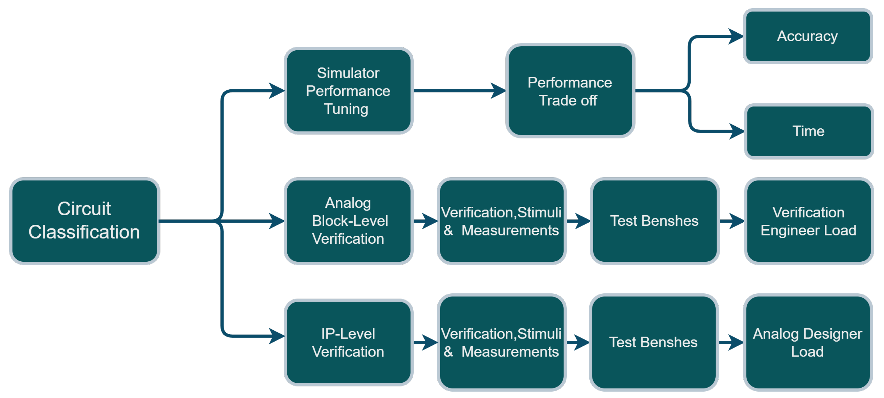
- Consider analog/mixed-signal verification. Within the context of the complicated process known as the verification of analog/mixed signals, dependable circuit classification (also known as circuit recognition) is one of the essential features that is required. Comparing a circuit’s output signal to a reference value, the expectation that the output will fall within a range of values is the last step in verifying an analog circuit that uses mixed signals. Without first understanding what this circuit symbolizes, it is impossible to make this comparison. This is why the classification of circuits or the identification of circuits is so essential [12,13,14].
- Consider layout generation. The ability to recognize/classify building blocks is an important capability supporting layout automation, as it provides one with a ground of optimization parameters of relevance for the layout process (e.g., expected heat generation, area, wire length, etc.) [1,2,3,6,7,8,9,10,11,20,21,22,23,24].
- REQ-1: A classification accuracy (or precision) that is very high, e.g., lying in a range between 97 to more than 99 percent.
- REQ-2: It shall be robust w.r.t. topology/architecture variations of circuits having the same label.
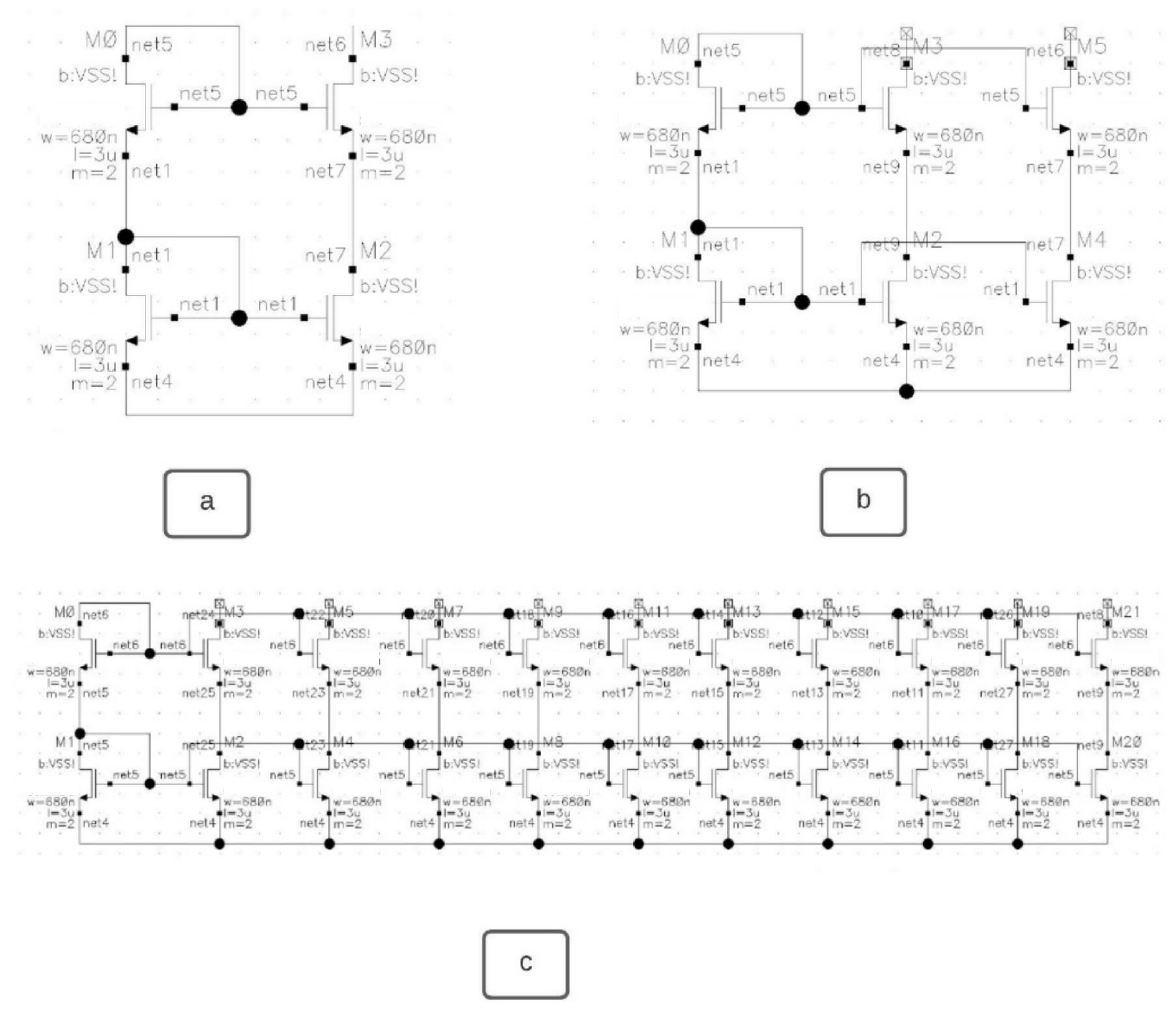
- REQ-3: It shall be robust w.r.t. to topology/architecture variations/extension related to banks (e.g., current mirror banks of different dimensions, etc.).
- REQ-4: It shall be robust to variations involving different transistor technologies uniformly or mixed in the same analog circuit structure (e.g., bipolar, NMOS, PMOS, etc.) in various samples of the datasets (for both training and testing) under the same label.
- REQ-5: It shall be robust to practically common imperfections of the training dataset(s) (e.g., amongst others, limited dataset size, unbalanced dataset, etc.).
- REQ-6: The concept shall be applicable, in principle, to each of the levels of analog circuits architectures or IPs (IP refers to intellectual property packages) such as, just for illustration, level 1 (i.e. that of the basic building blocks), level 2 (i.e., that of the functional blocks), level 3 (i.e., that of the modules), etc.
3. Comprehensive Critical Review of the Related State-of-the-Art
4. General Methodology Used for Building an Analog Circuits Classifier Pipeline
4.1. Proof of Concept Scenario and Dataset Issues
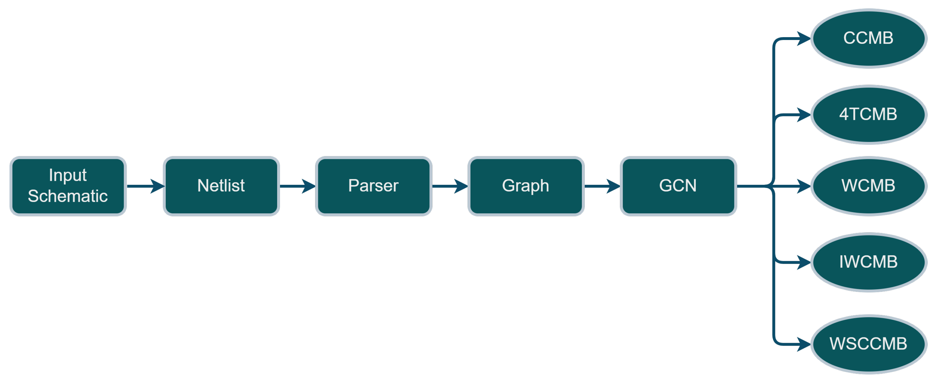
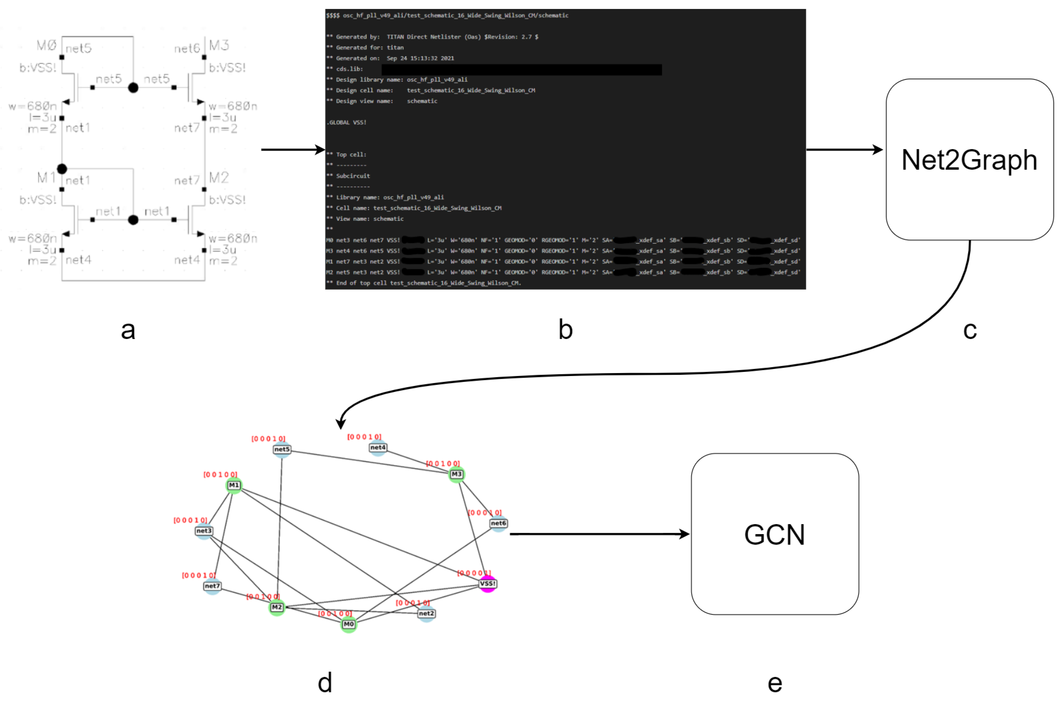
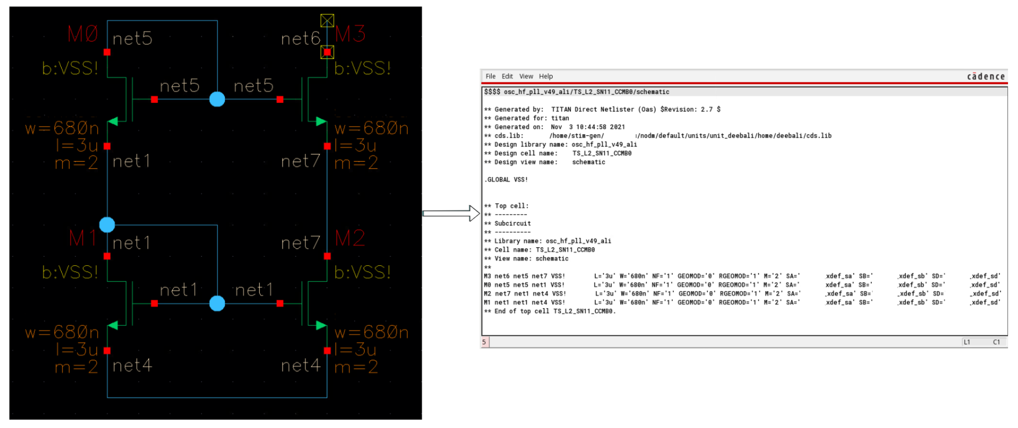
4.2. Preprocessing—The Parser
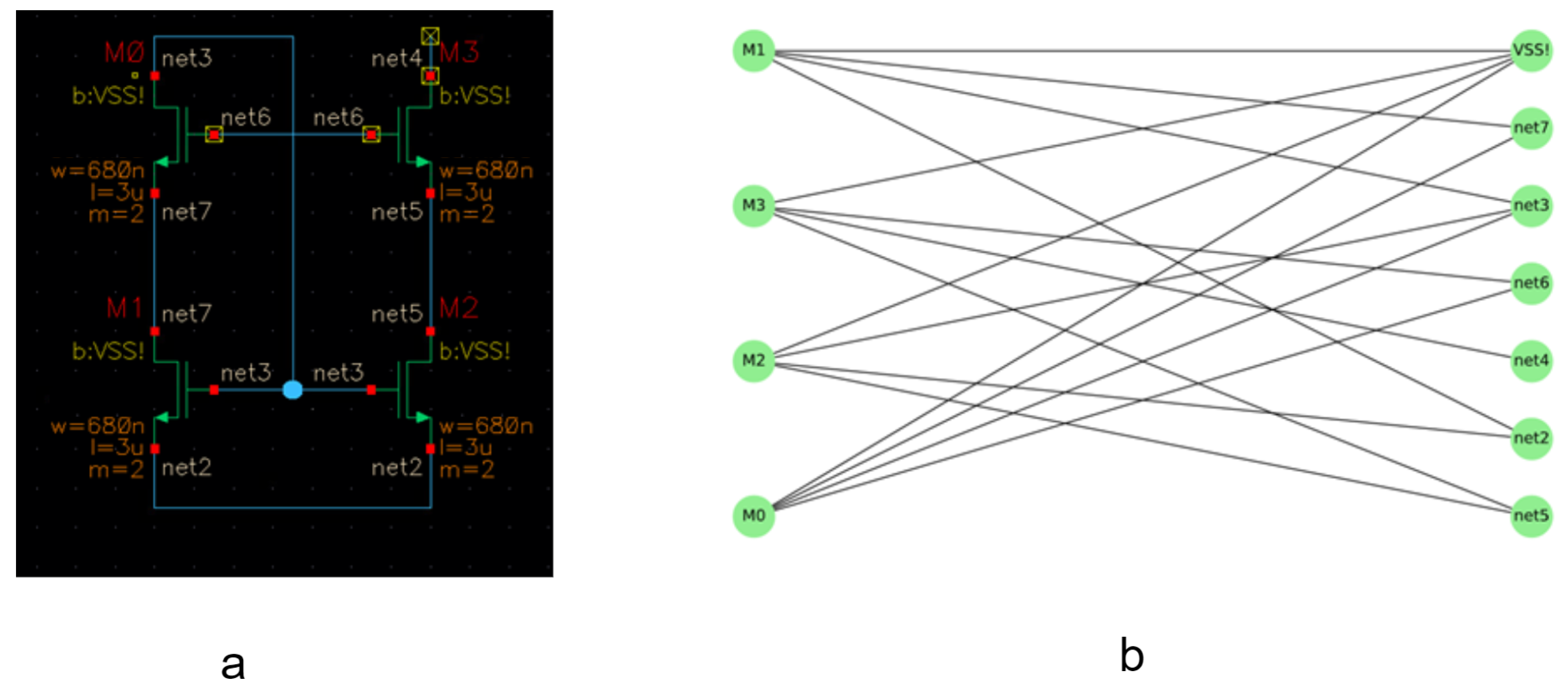
- Consider Level 0: This is the level consisting of the basic electronic elements such as transistors, capacitors, etc. These are interconnected through nets in the Cadence Virtuoso schematics and thereby constitute a level-0 graph. It does contain two types of nodes: the nets and the components. There is an edge between pair of nodes, whenever there exists a direct connection between them in the schematics. It is very important to notice that in most analog/mix circuits engineering processes, any circuit or circuit element of higher levels (level-1, level-2, level-3, etc.) is always and generally provided in form of a level-0 graph only. Indeed, the netlists generated for each of those circuits, independently of the level, is always described in form of a corresponding level-0 graph model.
- Consider Level 1: This is the level of the basic building blocks. Their schematics provided in Cadence Virtuoso do enable the netlist-based generation of their respective level-0 graph models. Thus, a classification (involving a GCN processor model) of level-1 entities will process their respective level-0 graph models.
- Consider Level 2: This is the level of the functional building blocks. Their schematics provided in Cadence Virtuoso do enable the netlist-based generation of their respective level-0 graph models. Thus, a classification (involving a GCN processor model) of level-2 entities will process their respective level-0 graph models.
- Consider Level 3: This is the level of the functional modules. Their schematics provided in Cadence Virtuoso do enable the netlist-based generation of their respective level-0 graph models. Thus, a classification (involving a GCN processor model) of level-3 entities will process their respective level-0 graphs models.
4.3. GCN Model
- The first option is to use spectral graph convolution graph neural networks (GCN), which handle non-homogeneous (w.r.t. size) input graphs by converting them to edge lists. They are called spatial GCN [44].
- The second option is to use either a vanilla GCN or a spectral GCN, and to face the limitation related to the fixed size of their inputs, we (one) perform(s) zero padding to unite graph sizes to the maximum graph corresponding to the biggest schematics within the dataset [44].
5. Dataset Collection, Transformation, and Preprocessing
5.1. Dataset Collection
5.2. Dataset Transformation
5.3. Dataset Preprocessing
6. A Robust GCN-Based Classifier Model—Design and Validation
- Spectral-based graph convolutional networks. Introduced by Bruna et al. [49], they are the first notable graph-based networks and do incorporate various spectral convolutional layers inspired by CNNs.
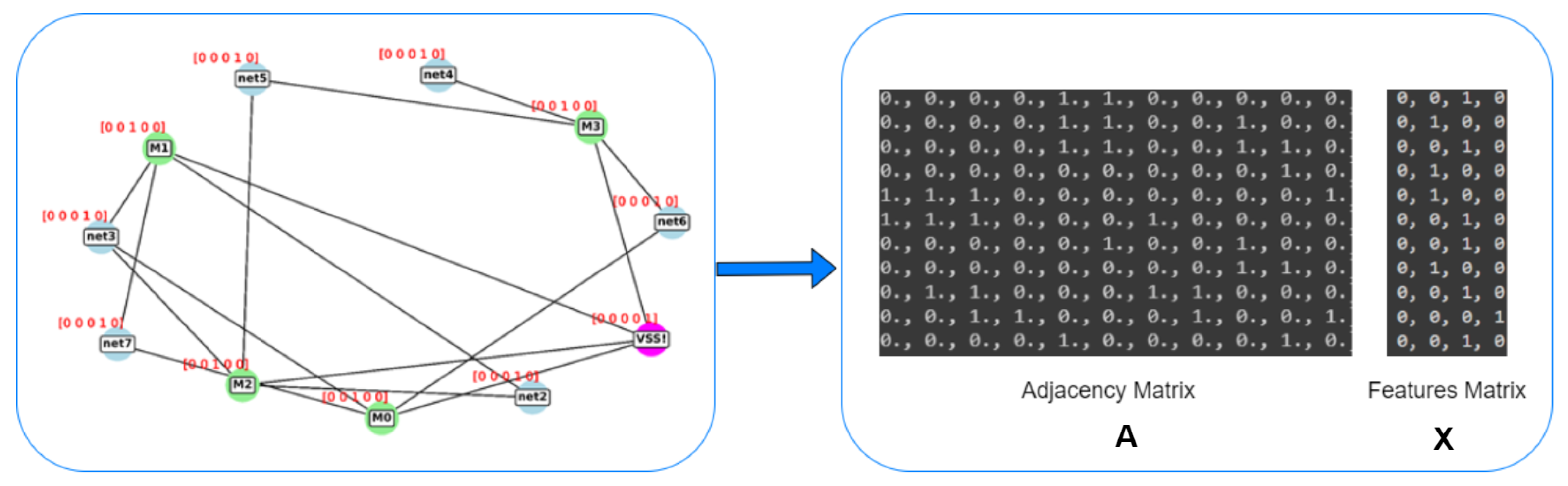
- Spatial-based graph convolutional networks. They were first introduced by Kipf et al. [41]. Kipf introduced a two-layer graph convolution network for semi-supervised node classification. Every node (i) in a graph has a feature vector x(i) which can be combined in a feature matrix X of dimensions n×d where n is: the number of nodes and d is the number of input features. An adjacency matrix A represents the graph structure or the respective connectivity.
- One-layer graph-convolution GCN architecture.
- Two-layer graph-convolution GCN architecture.
- Three-layer graph-convolution GCN architecture.
- Four-layer graph-convolution GCN architecture.
- Five-layer graph-convolution GCN architecture.
7. K-Fold Cross Validation
7.1. List of Scenarios
7.1.1. The 5 Folds Case
7.1.2. The 15 Folds Case
8. Addressing the Challenge of Limited Datasets through Innovative Data Augmentation Concepts for Better Training the GCN Classifier
8.1. Related Works
8.1.1. Node Augmentations
8.1.2. Edge Augmentations
8.1.3. Feature Augmentations
8.1.4. Subgraph Augmentation
9. Proposed Dataset Augmentation Method
9.1. Electrical Augmentation
- NMOS: 50 Schematics (original dataset).
- PMOS: 50 Schematics (first duplication).
- bipolar: 50 Schematics (second duplication).
9.2. Numerical Augmentation
9.2.1. Feature Matrix Augmentation
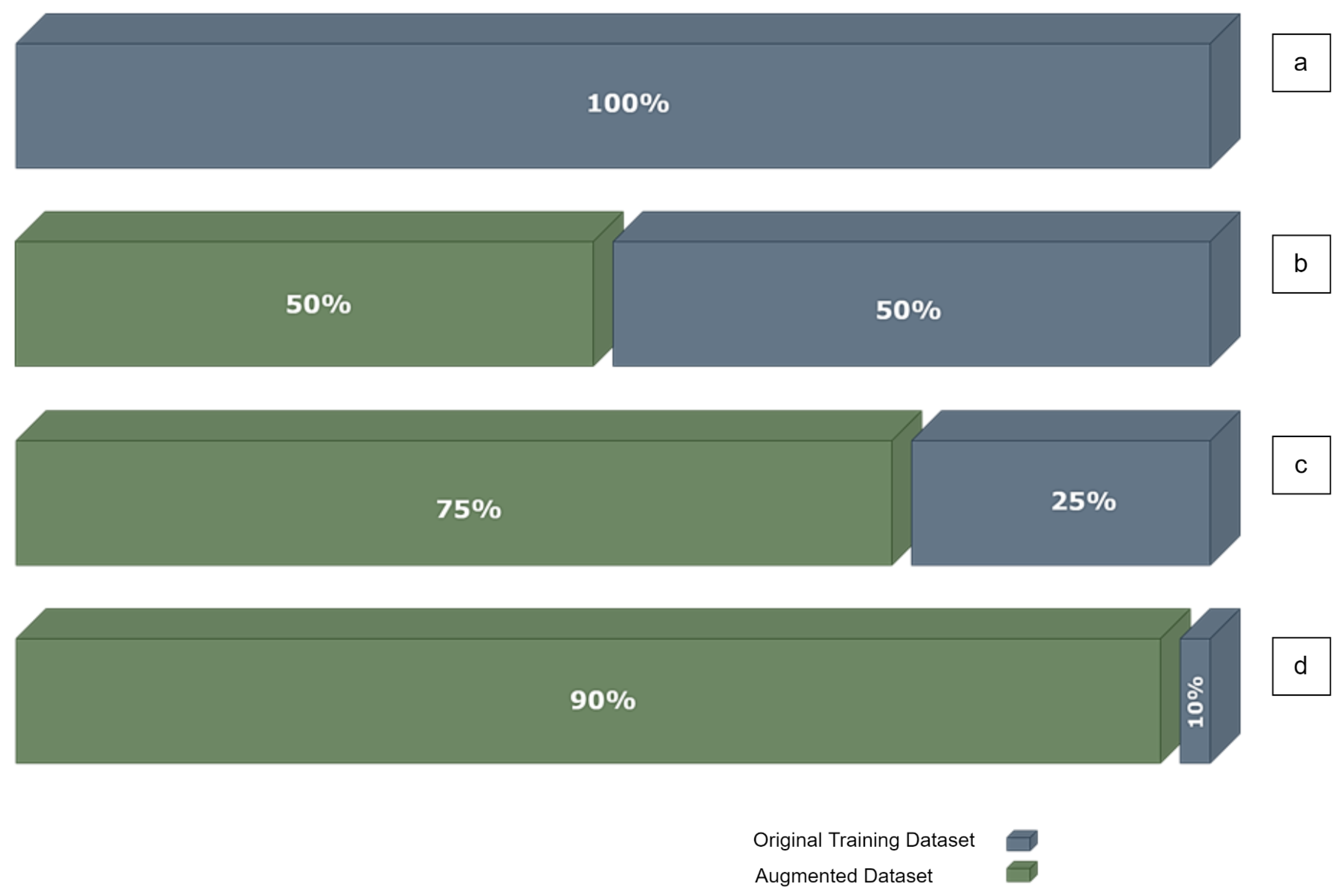
- SCENARIO 1: Using the whole training dataset TDS (i.e., 100%)
- SCENARIO 2: Reduced training data (a selection) to a portion of the original data; specifically to ½ of the original training dataset.
- SCENARIO 3: Reduced training data (a selection) to a portion of the original data; specifically to ¼ of the original training dataset.
- SCENARIO 4: Reduced training data (a selection) to a portion of the original data; specifically to 1/10 of the original training dataset.
- SCENARIO 5: Augment to compensate the missing data samples in scenario 2; shown in Figure 11b.
- SCENARIO 6: Augment to compensate the missing data samples in scenario 3; shown in Figure 11c.
- SCENARIO 7: Augment to compensate the missing data samples in scenario 4; shown in Figure 11d.
- Experiment-1: Add the same random number from the interval [0.001, 0.01] to all non-zeros elements in the feature matrix X to construct X2 as a new feature matrix of the same graph. Table 6 shows a performance comparison of different scenarios, numbered as explained above, where we take a part of the training set for training and we keep the same test dataset for testing. The first two lines show the mean accuracy for each dataset case, where we take for training half of the dataset, a quarter, then a tenth, and then test with the same test dataset of 50 graphs. As expected, the mean accuracy drops when the model has fewer data to train. The second two lines show the compensation we did with the augmented data as explained in Figure 11. The accuracy is better compared to the first two lines, but it is still far from the accuracy where we use the whole training dataset TDS for training. The division sign ‘/’ is used to refer to taking part of the dataset. For example, TDS/2 means half of the dataset TDS. The asterisk sign ‘*’ refers to the augmentation, and the number after it refers to the scale of augmentation, or how many replicas we do using the augmentation technique described in each experiment.

| Dataset | 1. TDS | 2. TDS/2 | 3. TDS/4 | 4. TDS/10 |
|---|---|---|---|---|
| Mean Accuracy reached after training with the reduced datasets | 90.50 ± 0.26 | 48.20 ± 0.52 | 40.05 ± 0.74 | 32.20 ± 0.54 |
| Augmented Dataset | 1. TDS | 5. (TDS/2)*2 | 6. (TDS/4)*4 | 7.(TDS/10)*10 |
| Mean Accuracy (in%) reached after testing the model training by the augmented datasets | 90.50 ± 0.26 | 50.54 ± 0.15 | 42.86 ± 0.25 | 30.19 ± 0.62 |
- Experiment-2: Add the same random number from the interval [0.001, 0.01] to all elements in the feature matrix X to construct X2. Table 7 is similar to Table 6 in terms of scenarios implemented and the numbers of scenarios were removed for simplicity. Table 7 shows that the accuracy (see Table 7) is worse than the first experiment (see Table 6). This means that adding a small random number to the zeros within the feature matrix does result in a some confusion to the model.
| Dataset | 1. TDS | 2. TDS/2 | 3. TDS/4 | 4. TDS/10 |
|---|---|---|---|---|
| Mean Accuracy reached after training with the reduced datasets | 90.50 ± 0.26 | 48.20 ± 0.52 | 40.05 ± 0.74 | 32.20 ± 0.54 |
| Augmented Dataset | 1. TDS | 5. (TDS/2)*2 | 6. (TDS/4)*4 | 7. (TDS/10)*10 |
| Mean Accuracy (in%) reached after testing the model training by the augmented datasets | 90.50 ± 0.26 | 37.61 ± 0.84 | 28.35 ± 0.55 | 22.70 ± 0.50 |
- Experiment-3: Add a random from the interval [0.001, 0.01] to each non-zero element (the random number will be different for each element of the feature matrix) in the feature matrix X to construct X2. Table 8 shows a big enhancement compared to the first two experiments. The new augmented feature matrices have the same structure as the original ones with the small tuning of the non-zero elements, and apparently, this helped the model cope with the new samples of the test dataset.
| Dataset | 1. TDS | 2. TDS/2 | 3. TDS/4 | 4. TDS/10 |
|---|---|---|---|---|
| Mean Accuracy reached after training with the reduced datasets | 90.50 ± 0.26 | 48.20 ± 0.52 | 40.05 ± 0.74 | 32.20 ± 0.54 |
| Augmented Dataset | 1. TDS | 5. (TDS/2)*2 | 6. (TDS/4)*4 | 7. (TDS/10)*10 |
| Mean Accuracy (in%) reached after testing the model training by the augmented datasets | 90.50 ± 0.26 | 76.60 ± 0.32 | 58.75 ± 0.34 | 40.80 ± 0.50 |
- Experiment-4: Add a random from the interval [0.001, 0.01] to each element (the random number will be different for each element of the feature matrix) in the feature matrix X to construct X2. Table 9 shows a decrease in the performance of the model for the same reason in experiment 2, which is adding random numbers to the zero elements of the feature matrix.
| Dataset | 1. TDS | 2. TDS/2 | 3. TDS/4 | 4. TDS/10 |
|---|---|---|---|---|
| Mean Accuracy reached after training with the reduced datasets | 90.50 ± 0.26 | 48.20 ± 0.52 | 40.05 ± 0.74 | 32.20 ± 0.54 |
| Augmented Dataset | 1. TDS | 5. (TDS/2)*2 | 6. (TDS/4)*4 | 7. (TDS/10)*10 |
| Mean Accuracy (in%) reached after testing the model training by the augmented datasets | 90.50 ± 0.26 | 40.33 ± 0.82 | 32.22 ± 0.37 | 24.70 ± 0.60 |
| Experiment 1 | ||||
| Dataset | TDS | TDS/2 | TDS/4 | TDS/10 |
| Mean Accuracy | 90.50 ± 0.26 | 48.20 ± 0.52 | 40.05 ± 0.74 | 32.20 ± 0.54 |
| Augmented Dataset | TDS | (TDS/2)*2 | (TDS/4)*4 | (TDS/10)*10 |
| Mean Accuracy | 90.50 ± 0.26 | 58.50 ± 0.72 | 46.32 ± 0.38 | 32.56 ± 0.43 |
| Experiment 2 | ||||
| Dataset | TDS | TDS/2 | TDS/4 | TDS/10 |
| Mean Accuracy | 90.50 ± 0.26 | 48.20 ± 0.52 | 40.05 ± 0.74 | 32.20 ± 0.54 |
| Augmented Dataset | TDS | (TDS/2)*2 | (TDS/4)*4 | (TDS/10)*10 |
| Mean Accuracy | 90.50 ± 0.26 | 36.54 ± 0.15 | 26.75 ± 0.78 | 20.95 ± 0.84 |
| Experiment 3 | ||||
| Dataset | TDS | TDS/2 | TDS/4 | TDS/10 |
| Mean Accuracy | 90.50 ± 0.26 | 48.20 ± 0.52 | 40.05 ± 0.74 | 32.20 ± 0.54 |
| Augmented Dataset | TDS | (TDS/2)*2 | (TDS/4)*4 | (TDS/10)*10 |
| Mean Accuracy | 90.50 ± 0.26 | 78.60 ± 0.45 | 60.46 ± 0.55 | 44.85 ± 0.44 |
| Experiment 4 | ||||
| Dataset | TDS | TDS/2 | TDS/4 | TDS/10 |
| Mean Accuracy | 90.50 ± 0.26 | 48.20 ± 0.52 | 40.05 ± 0.74 | 32.20 ± 0.54 |
| Augmented Dataset | TDS | (TDS/2)*2 | (TDS/4)*4 | (TDS/10)*10 |
| Mean Accuracy | 90.50 ± 0.26 | 37.88 ± 0.46 | 25.45 ± 0.87 | 21.44 ± 0.35 |
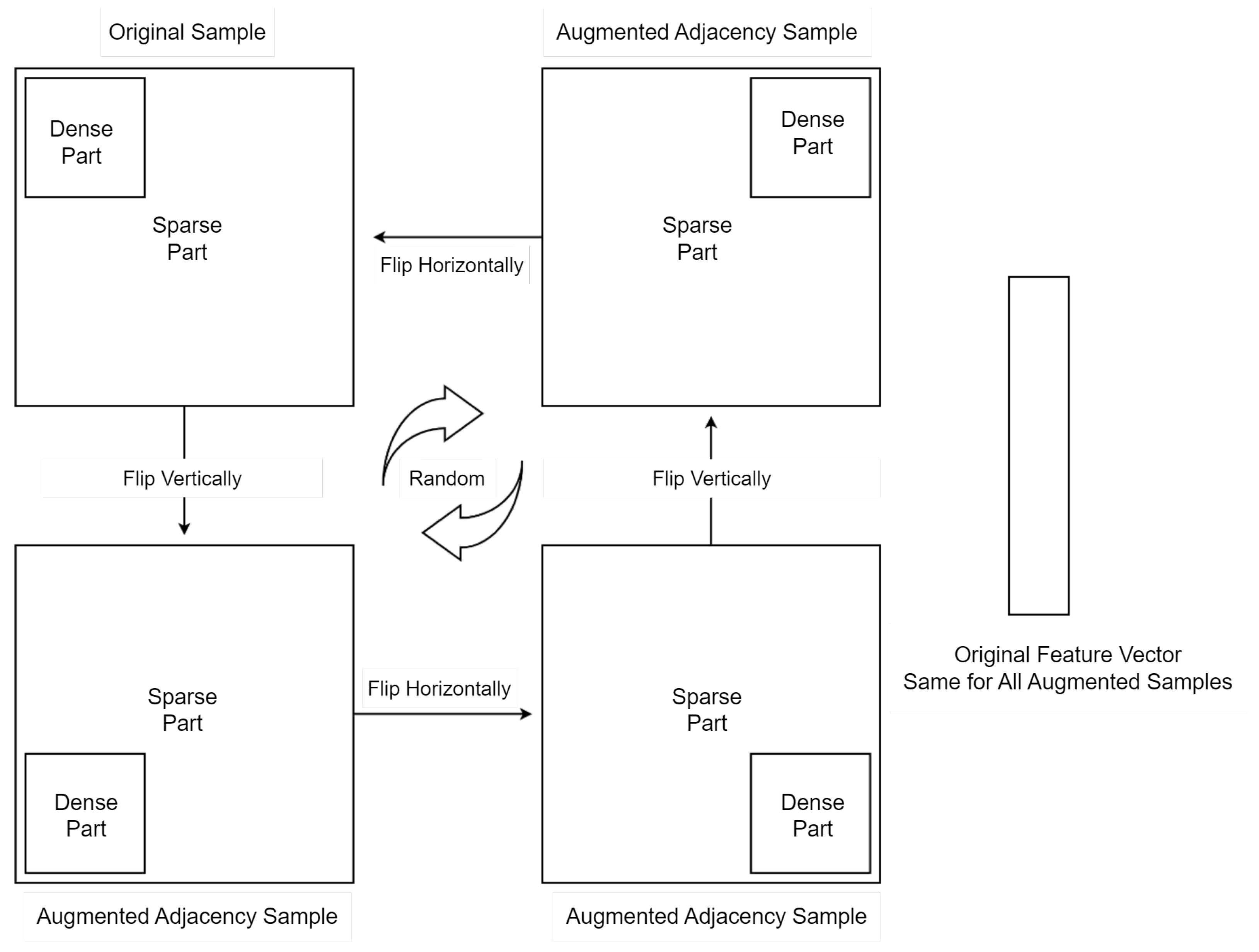
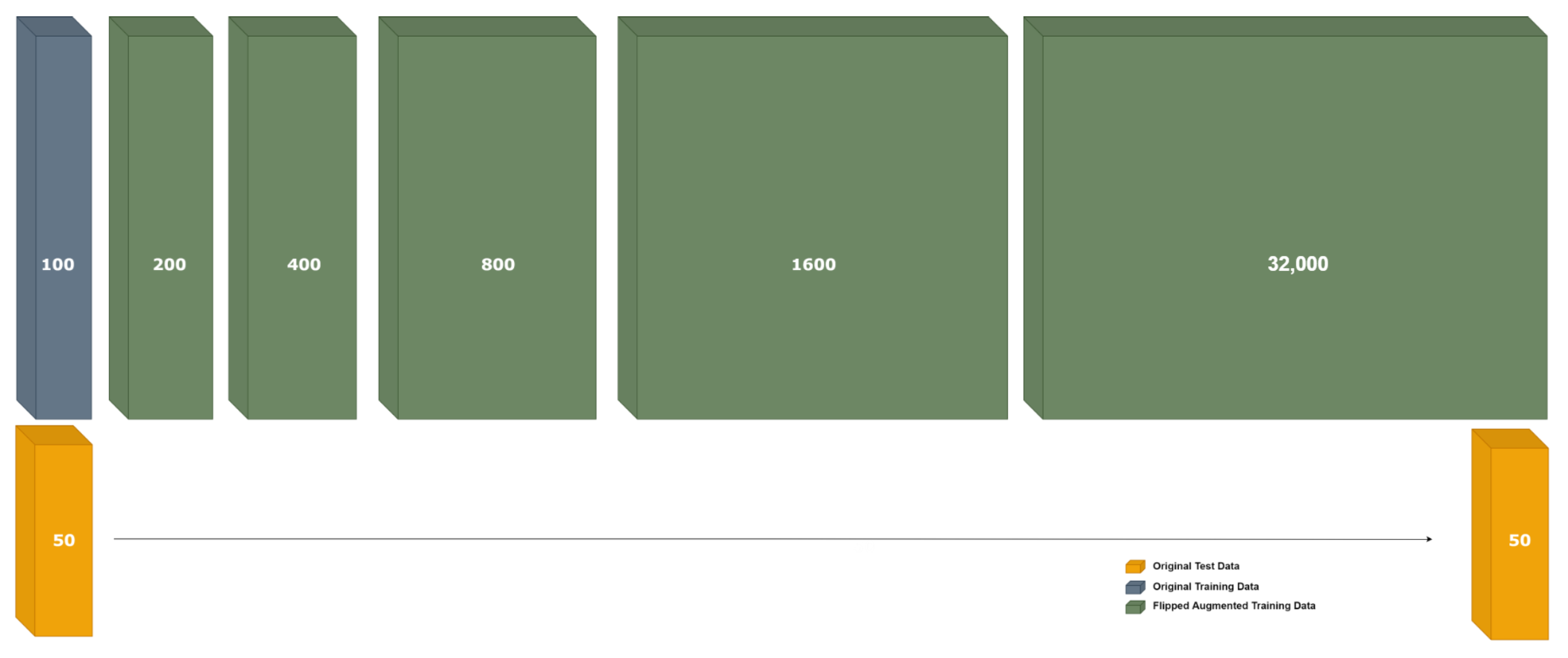
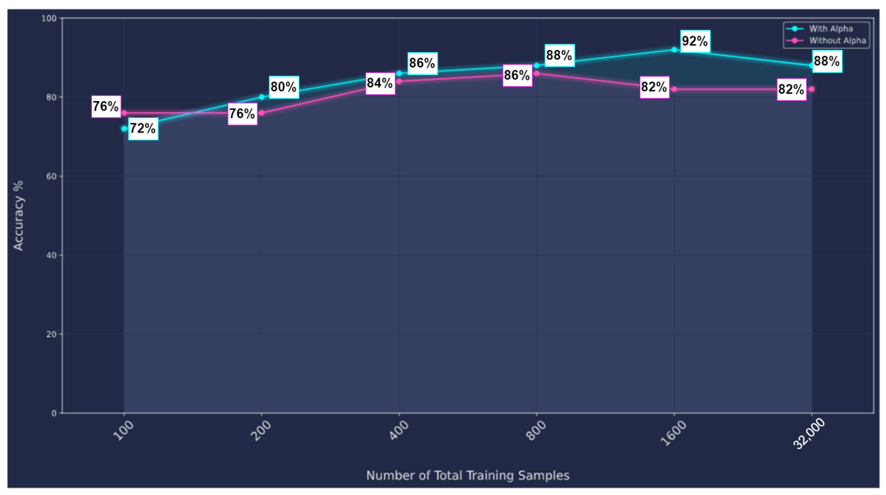
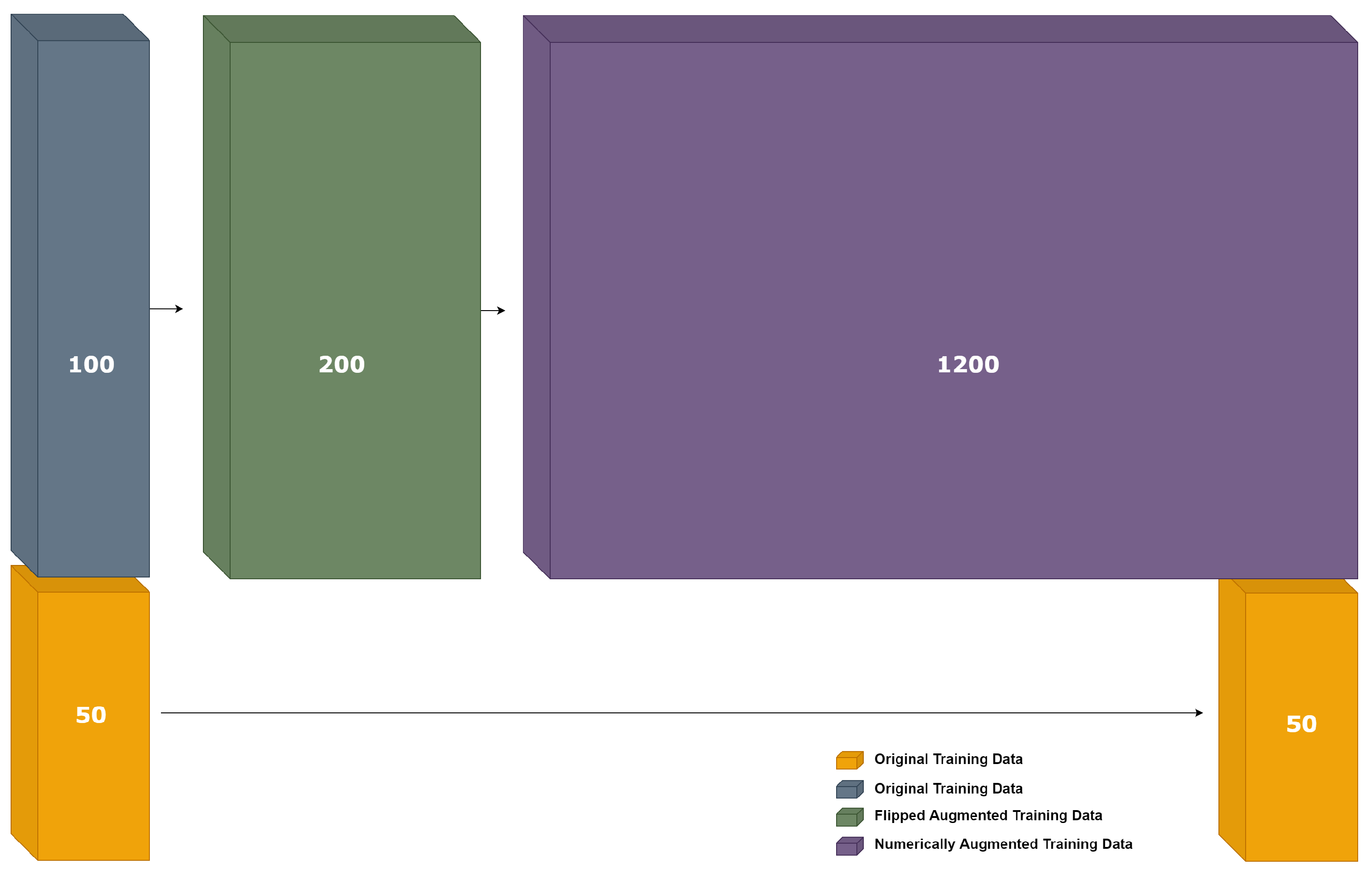
9.2.2. Dataset Augmentation by Flipping
- Without Alpha; applying the flipping augmentation on the original feature vector, and checking the performance enhancement by increasing the number of samples.
- With Alpha; we multiplied each feature vector by a unique alpha sampled uniformly from [0.0001, 0.001].
9.2.3. Multi-Stage Augmentation
9.2.4. Hyperphysical Augmentation
9.2.5. Numerical Augmentation of the Hyperphysically Augmented Dataset
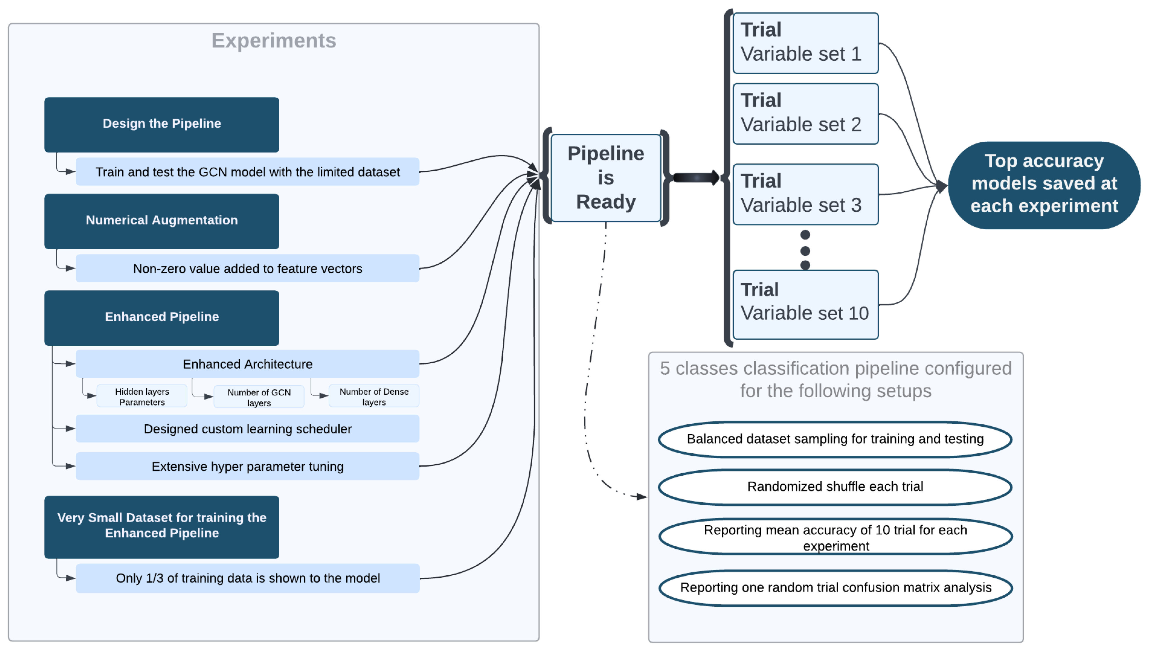
10. Experiments Anatomy for the Different Pipelines
- The first pipeline was designed to train and test the GCN model using a limited dataset of 150 graphs. The dataset was split into 100 graphs for training and 50 for testing. The classes were balanced, since the samples have different sizes.
- In order to enhance the preliminary classification accuracy, numerical augmentations were applied. As explained in Section 9.2, four experiments were made to add small value to the elements of the feature matrix. The third experiment of adding a random to the non-zero elements of the feature matrix gave the best results among the four experiments.
- Enhanced Pipeline: we have enhanced the pipeline to have more reliable and consistent results by performing the following changes:
- Enhanced Architecture: improving the hidden layers’ parameters, the number of GCN layers, and the number of fully connected layers.
- Designing the custom learning scheduler: we have chosen an exponential decay: It divides the learning rate for every epoch by the same percentage (%). This indicates that the learning rate will gradually decline over time, spending more epochs with a lower value but never reaching zero.
- Extensive hyperparameter tuning: fix all parameters and optimize one to check the impact of tuning the respective hyperparameters on the performance results.
- Small dataset with enhanced pipeline: only 1/3 of training data were shown to the model to check the enhancement achieved by applying the various augmentation techniques on the small training dataset.
- Balanced dataset sampling for training and testing.
- Randomized shuffle each trial.
- Reporting mean accuracy of 10 trials for each experiment.
- Reporting a confusion matrix to analyze the analysis of the results.
11. Qualitative and Conceptual Comparison of the Concept Presented in This Paper with a Selection of the Most Relevant Related Works, Especially from the Perspective of the “Comprehensive Requirements Dossier” at Stake
12. Conclusions
Author Contributions
Funding
Institutional Review Board Statement
Informed Consent Statement
Data Availability Statement
Acknowledgments
Conflicts of Interest
References
- Eick, M.; Strasser, M.; Lu, K.; Schlichtmann, U.; Graeb, H.E. Comprehensive generation of hierarchical placement rules for analog integrated circuits. IEEE Trans. Comput.-Aided Des. Integr. Circuits Syst. 2011, 30, 180–193. [Google Scholar] [CrossRef]
- Mina, R.; Jabbour, C.; Sakr, G.E. A review of machine learning techniques in analog integrated circuit design automation. Electronics 2022, 11, 435. [Google Scholar] [CrossRef]
- Moore, G.E. Cramming more components onto integrated circuits. Proc. IEEE Inst. Electr. Electron. Eng. 1998, 86, 82–85. [Google Scholar] [CrossRef]
- Kunal, K.; Dhar, T.; Madhusudan, M.; Poojary, J.; Sharma, A.; Xu, W.; Burns, S.M.; Hu, J.; Harjani, R.; Sapatnekar, S.S. GANA: Graph convolutional network based automated netlist annotation for analog circuits. In Proceedings of the 2020 Design, Automation & Test in Europe Conference & Exhibition (DATE), Grenoble, France, 9–13 March 2020. [Google Scholar]
- Hong, X.; Lin, T.; Shi, Y.; Gwee, B.H. ASIC Circuit Netlist Recognition Using Graph Neural Network. In Proceedings of the 2021 IEEE International Symposium on the Physical and Failure Analysis of Integrated Circuits (IPFA), Singapore, 15 September–15 October 2021. [Google Scholar]
- Graeb, H.; Zizala, S.; Eckmueller, J.; Antreich, K. The sizing rules method for analog integrated circuit design. In Proceedings of the IEEE/ACM International Conference on Computer Aided Design, ICCAD 2001, San Jose, CA, USA, 4–8 November 2001. IEEE/ACM Digest of Technical Papers (Cat. No.01CH37281). [Google Scholar]
- Massier, T.; Graeb, H.; Schlichtmann, U. The sizing rules method for CMOS and bipolar analog integrated circuit synthesis. IEEE Trans. Comput.-Aided Des. Integr. Circuits Syst. 2008, 27, 2209–2222. [Google Scholar] [CrossRef]
- Debyser, G.; Gielen, G. Efficient analog circuit synthesis with simultaneous yield and robustness optimization. In Proceedings of the 1998 IEEE/ACM International Conference on Computer-Aided Design—ICCAD ’98, San Jose, CA, USA, 8–12 November 1998. [Google Scholar]
- Mandal, P.; Visvanathan, V. CMOS op-amp sizing using a geometric programming formulation. IEEE Trans. Comput.-Aided Des. Integr. Circuits Syst. 2001, 20, 22–38. [Google Scholar] [CrossRef]
- Gerlach, A.; Scheible, J.; Rosahl, T.; Eitrich, F.-T. A generic topology selection method for analog circuits with embedded circuit sizing demonstrated on the OTA example. In Proceedings of the Design, Automation & Test in Europe Conference & Exhibition (DATE), Lausanne, Switzerland, 27–31 March 2017. [Google Scholar]
- Gray, P.R.; Hurst, P.J.; Lewis, S.H.; Meyer, R.G. Analysis and Design of Analog Integrated Circuits, 6th ed.; Wiley: New York, NY, USA, 2020. [Google Scholar]
- Balasubramanian, S.; Hardee, P. Solutions for mixed-signal soc verification using real number models. In Cadence Design Systems; Cadence: San Jose, CA, USA, 2013; pp. 1–4. [Google Scholar]
- Karnane, K.; Curtis, G.; Goering, R. Solutions for mixed-signal SoC verification. In Cadence Design Systems; Cadence: San Jose, CA, USA, 2009. [Google Scholar]
- Chen, J.; Henrie, M.; Mar, M.F.; Nizic, M. Mixed-Signal Methodology Guide; Lulu.com: Morrisville, NC, USA, 2012; pp. 13–14. 76–82. [Google Scholar]
- Massier, T. On the Structural Analysis of CMOS and Bipolar Analog Integrated Circuits. Ph.D. Thesis, Technische Universität München, Munich, Germany, 2010. [Google Scholar]
- Yao, Y.; Holder, L. Scalable svm-based classification in dynamic graphs. In Proceedings of the 2014 IEEE International Conference on Data Mining, Shenzhen, China, 14–17 December 2014. [Google Scholar]
- Li, G.; Semerci, M.; Yener, B.; Zaki, M.J. Graph classification via topological and label attributes. In Proceedings of the 9th International Workshop on Mining and Learning with Graphs (MLG), San Diego, CA, USA, 17 July 2011; Volume 2. [Google Scholar]
- Ohlrich, M.; Ebeling, C.; Ginting, E.; Sather, L. Subgemini: Identifying subcircuits using a fast subgraph isomorphism algorithm. In Proceedings of the 30th International Design Automation Conference, Dallas, TX, USA, 14–18 June 1993; pp. 14–18. [Google Scholar]
- Zhang, M.; Cui, Z.; Neumann, M.; Chen, Y. An end-to-end deep learning architecture for graph classification. In Proceedings of the AAAI Conference on Artificial Intelligence, New Orleans, LA, USA, 2–7 February 2018; Volume 32. [Google Scholar]
- Lavagno, L.; Martin, G.; Scheffer, L. Electronic Design Automation for Integrated Circuits Handbook—2 Volume Set; CRC Press: Boca Raton, FL, USA, 2006. [Google Scholar]
- Toledo, P.; Rubino, R.; Musolino, F.; Crovetti, P. Re-thinking analog integrated circuits in digital terms: A New Design concept for the IoT era. IEEE Trans. Circuits Syst. II Express Briefs 2021, 68, 816–822. [Google Scholar] [CrossRef]
- Hakhamaneshi, K.; Werblun, N.; Abbeel, P.; Stojanovic, V. BagNet: Berkeley analog generator with layout optimizer boosted with deep neural networks. In Proceedings of the 2019 IEEE/ACM International Conference on Computer-Aided Design (ICCAD), Westminster, CO, USA, 4–7 November 2019. [Google Scholar]
- Wei, P.-H.; Murmann, B. Analog and mixed-signal layout automation using digital place-and-route tools. IEEE Trans. Very Large Scale Integr. VLSI Syst. 2021, 29, 1838–1849. [Google Scholar] [CrossRef]
- Ahmad, T.; Jin, L.; Lin, L.; Tang, G. Skeleton-based action recognition using sparse spatio-temporal GCN with edge effective resistance. Neurocomputing 2021, 423, 389–398. [Google Scholar] [CrossRef]
- Liang, C.; Fang, Z.; Chen, C.-Z. Method for analog-mixed signal design verification and model calibration. In Proceedings of the 2015 China Semiconductor Technology International Conference, Shanghai, China, 15–16 March 2015. [Google Scholar]
- Jiao, F.; Montano, S.; Ferent, C.; Doboli, A.; Doboli, S. Analog circuit design knowledge mining: Discover-ing topological similarities and uncovering design reasoning strategies. IEEE Trans. Comput.-Aided Des. Integr. Circuits Syst. 2015, 34, 1045–1058. [Google Scholar] [CrossRef]
- Van der Plas, G.; Debyser, G.; Leyn, F.; Lampaert, K.; Vandenbussche, J.; Gielen, G.G.; Sansen, W.; Veselinovic, P.; Leenarts, D. AMGIE-A synthesis environment for CMOS analog integrated circuits. IEEE Trans. Comput.-Aided Des. Integr. Circuits Syst. 2001, 20, 1037–1058. [Google Scholar] [CrossRef]
- Chanak, T.S. Netlist Processing for Custom Vlsi via Pattern Matching; Stanford University: Stanford, CA, USA, 1995. [Google Scholar]
- Pelz, G.; Roettcher, U. Pattern matching and refinement hybrid approach to circuit comparison. IEEE Trans. Comput.-Aided Des. Integr. Circuits Syst. 1994, 13, 264–276. [Google Scholar] [CrossRef]
- Kim, W.; Shin, H. Hierarchical LVS based on hierarchy rebuilding. In Proceedings of the 1998 Asia and South Pacific Design Automation Conference, Yokohama, Japan, 13 February 1998. [Google Scholar]
- Rubanov, N. SubIslands: The probabilistic match assignment algorithm for subcircuit recognition. IEEE Trans. Comput.-Aided Des. Integr. Circuits Syst. 2003, 22, 26–38. [Google Scholar] [CrossRef]
- Rubanov, N. Fast and accurate identifying subcircuits using an optimization based technique. In Proceedings of the SCS 2003, International Symposium on Signals, Circuits and Systems, Proceedings (Cat. No.03EX720), Iasi, Romania, 10–11 July 2003. [Google Scholar]
- Rubanov, N. Bipartite graph labeling for the subcircuit recognition problem. In Proceedings of the ICECS 2001 8th IEEE International Conference on Electronics, Circuits and Systems (Cat. No.01EX483), Malta, Malta, 2–5 September 2001. [Google Scholar]
- Conn, A.R.; Elfadel, I.M.; Molzen, W.W., Jr.; O’brien, P.R.; Strenski, P.N.; Visweswariah, C.; Whan, C.B. Gradient-based optimization of custom circuits using a static-timing formulation. In Proceedings of the 1999 Design Automation Conference (Cat. No. 99CH36361), New Orleans, LA, USA, 21–25 June 1999. [Google Scholar]
- Rubanov, N. A high-performance subcircuit recognition method based on the nonlinear graph optimization. IEEE Trans. Comput.-Aided Des. Integr. Circuits Syst. 2006, 25, 2353–2363. [Google Scholar] [CrossRef]
- Yang, L.; Shi, C.-J.R. FROSTY: A fast hierarchy extractor for industrial CMOS circuits. In Proceedings of the ICCAD-2003, International Conference on Computer Aided Design (IEEE Cat. No.03CH37486), San Jose, CA, USA, 9–13 November 2003. [Google Scholar]
- Meissner, M.; Hedrich, L. FEATS: Framework for explorative analog topology synthesis. IEEE Trans. Comput.-Aided Des. Integr. Circuits Syst. 2015, 34, 213–226. [Google Scholar] [CrossRef]
- Wu, P.-H.; Lin, M.P.-H.; Chen, T.-C.; Yeh, C.-F.; Li, X.; Ho, T.-Y. A novel analog physical synthesis method-ology integrating existent design expertise. IEEE Trans. Comput.-Aided Des. Integr. Circuits Syst. 2015, 34, 199–212. [Google Scholar] [CrossRef]
- Li, H.; Jiao, F.; Doboli, A. Analog circuit topological feature extraction with unsupervised learning of new sub-structures. In Proceedings of the 2016 Design, Automation & Test in Europe Conference & Exhibition (DATE), Dresden, Germany, 14–18 March 2016. [Google Scholar]
- Liou, G.-H.; Wang, S.-H.; Su, Y.-Y.; Lin, M.P.-H. Classifying analog and digital circuits with machine learning techniques toward mixed-signal design automation. In Proceedings of the 2018 15th International Conference on Synthesis, Modeling, Analysis and Simulation Methods and Applications to Circuit Design (SMACD), Prague, Czech Republic, 2–5 July 2018. [Google Scholar]
- Kipf, T.N.; Welling, M. Semi-supervised classification with graph convolutional networks. arXiv 2016, arXiv:1609.02907. [Google Scholar]
- Hamilton, W.L.; Ying, R.; Leskovec, J. Representation learning on graphs: Methods and applications. arXiv 2017, arXiv:1709.05584. [Google Scholar]
- Neuner, M.; Abel, I.; Graeb, H. Library-free structure recognition for analog circuits. In Proceedings of the 2021 Design, Automation & Test in Europe Conference & Exhibition (DATE), Grenoble, France, 1–5 February 2021. [Google Scholar]
- Wu, Z.; Pan, S.; Chen, F.; Long, G.; Zhang, C.; Yu, P.S. A comprehensive survey on Graph Neural Networks. IEEE Trans. Neural Netw. Learn. Syst. 2021, 32, 4–24. [Google Scholar] [CrossRef]
- Zhang, S.; Tong, H.; Xu, J.; Maciejewski, R. Graph convolutional networks: A comprehensive review. Comput. Soc. Netw. 2019, 6, 1–23. [Google Scholar] [CrossRef]
- Leek, E.C.; Leonardis, A.; Heinke, D. Deep neural networks and image classification in biological vision. Vis. Res. 2022, 197, 108058. [Google Scholar] [CrossRef]
- Zambrano, B.; Strangio, S.; Rizzo, T.; Garzón, E.; Lanuzza, M.; Iannaccone, G. All-Analog Silicon Integration of Image Sensor and Neural Computing Engine for Image Classification. IEEE Access 2022, 10, 94417–94430. [Google Scholar] [CrossRef]
- Cao, P.; Zhu, Z.; Wang, Z.; Zhu, Y.; Niu, Q. Applications of graph convolutional networks in computer vision. Neural Comput. Appl. 2022, 34, 13387–13405. [Google Scholar] [CrossRef]
- Bruna, J.; Zaremba, W.; Szlam, A.; LeCun, Y. Spectral networks and locally connected networks on graphs. arXiv 2013, arXiv:1312.6203. [Google Scholar]
- Chen, J.; Ma, T.; Xiao, C. FastGCN: Fast learning with graph convolutional networks via importance sampling. arXiv 2018, arXiv:1801.10247. [Google Scholar]
- Chen, J.; Zhu, J.; Song, L. Stochastic training of graph convolutional networks with variance reduction. arXiv 2017, arXiv:1710.10568. [Google Scholar]
- Huang, W.; Zhang, T.; Rong, Y.; Huang, J. Adaptive sampling towards fast graph representation learning. arXiv 2018, arXiv:1809.05343. [Google Scholar]
- Levie, R.; Monti, F.; Bresson, X.; Bronstein, M.M. CayleyNets: Graph convolutional neural networks with complex rational spectral filters. IEEE Trans. Signal Process. 2019, 67, 97–109. [Google Scholar] [CrossRef]
- Dwivedi, V.P.; Joshi, C.K.; Laurent, T.; Bengio, Y.; Bresson, X. Benchmarking Graph Neural Networks. arXiv 2020, arXiv:2003.00982. [Google Scholar]
- Ashfaque, J.M.; Iqbal, A. Introduction to Support Vector Machines and Kernel Methods. 2019. Available online: https://www.researchgate.net/publication/332370436 (accessed on 16 April 2022).
- KarlRosaen. Available online: http://karlrosaen.com/ml/learning-log/2016-06-20/ (accessed on 9 December 2022).
- Zhao, T.; Liu, G.; Günnemann, S.; Jiang, M. Graph Data Augmentation for Graph Machine Learning: A Survey. arXiv 2022, arXiv:2202.08871. [Google Scholar]
- Kong, K.; Li, G.; Ding, M.; Wu, Z.; Zhu, C.; Ghanem, B.; Taylor, G.; Goldstein, T. Flag: Adversarial data augmentation for graph neural networks. arXiv 2020, arXiv:2010.09891. [Google Scholar]
- You, Y.; Chen, T.; Sui, Y.; Chen, T.; Wang, Z.; Shen, Y. Graph contrastive learning with augmentations. Adv. Neural Inf. Process. Syst. 2020, 33, 5812–5823. [Google Scholar]
- Guo, H.; Mao, Y. ifMixup: Towards Intrusion-Free Graph Mixup for Graph Classification. arXiv 2021, arXiv:2110.09344. [Google Scholar]
- You, Y.; Chen, T.; Shen, Y.; Wang, Z. Graph contrastive learning automated. In Proceedings of the 38th International Conference on Machine Learning, Virtual Event, 18–24 July 2021. [Google Scholar]
- Song, R.; Giunchiglia, F.; Zhao, K.; Xu, H. Topological regularization for graph neural networks augmentation. arXiv 2021, arXiv:2104.02478. [Google Scholar]
- Liu, S.; Ying, R.; Dong, H.; Li, L.; Xu, T.; Rong, Y.; Zhao, P.; Huang, J.; Wu, D. Local Augmentation for Graph Neural Networks. arXiv 2021, arXiv:2109.03856. [Google Scholar]
- Gibson, J.B.; Hire, A.C.; Hennig, R.G. Data-Augmentation for Graph Neural Network Learning of the Relaxed Energies of Unrelaxed Structures. arXiv 2022, arXiv:2202.13947. [Google Scholar] [CrossRef]
- Zhao, T.; Liu, Y.; Neves, L.; Woodford, O.; Jiang, M.; Shah, N. Data augmentation for graph neural networks. arXiv 2020, arXiv:2006.06830. [Google Scholar] [CrossRef]
- Wang, Y.; Wang, W.; Liang, Y.; Cai, Y.; Hooi, B. Graphcrop: Subgraph cropping for graph classification. arXiv 2020, arXiv:2009.10564. [Google Scholar]
- Zhou, J.; Shen, J.; Xuan, Q. Data augmentation for graph classification. In Proceedings of the 29th ACM International Conference on Information & Knowledge Management, Virtual, 19–23 October 2020. [Google Scholar]
- Sun, M.; Xing, J.; Wang, H.; Chen, B.; Zhou, J. MoCL: Data-driven molecular fingerprint via knowledge-aware contrastive learning from molecular graph. In Proceedings of the 27th ACM SIGKDD Conference on Knowledge Discovery & Data Mining, Virtual, 14–18 August 2021. [Google Scholar]
- Wang, Y.; Wang, W.; Liang, Y.; Cai, Y.; Hooi, B. Mixup for node and graph classification. In Proceedings of the Web Conference 2021, Ljubljana, Slovenia, 19–23 April 2021. [Google Scholar]
- Park, J.; Shim, H.; Yang, E. Graph transplant: Node saliency-guided graph mixup with local structure preservation. In Proceedings of the AAAI Conference on Artificial Intelligence, Arlington, VA, USA, 17–19 November 2022; Volume 36. No. 7. [Google Scholar]
- Chen, D.; Lin, Y.; Li, W.; Li, P.; Zhou, J.; Sun, X. Measuring and relieving the over-smoothing problem for graph neural networks from the topological view. In Proceedings of the AAAI Conference on Artificial Intelligence, New York, NY, USA, 7–12 February 2020; Volume 34. [Google Scholar]


| Most Relevant Related Works | Classification Accuracy in Range 97–99% (REQ-1) | Robustness w.r.t. Architecture Variations (REQ-2) | Robustness w.r.t. Architecture Extension through Banks (REQ-3) | Robustness w.r.t. Transistor Technologies Variations (REQ.4) | Robustness w.r.t. Training Dataset Imperfections (REQ-5) | Applicability to Higher Levels of AMS IP Stacks |
|---|---|---|---|---|---|---|
| Kunal et al. [4] | Yes | Yes | No | No | No | Yes, possibly |
| Hong et al. [5] | Yes | Yes | No | No | No | Yes, possibly |
| Zhang et al. [19] | Yes | Yes | No | No | No | Yes, possibly |
| Ahmad et al. [24] | Yes | Yes | No | No | No | Yes, possibly |
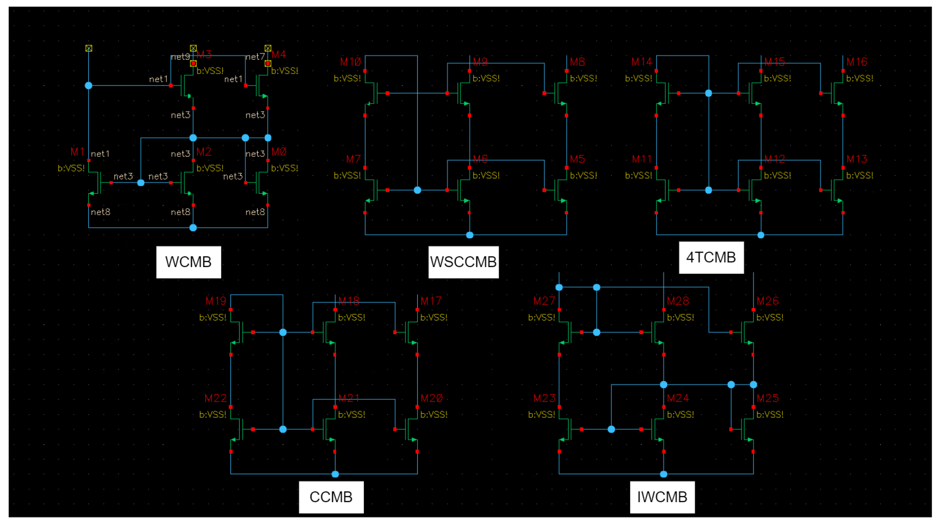
| Wide Swing Cascode Current Mirror Bank | Cascode Current Mirror Bank | 4 Transistor Current Mirror Bank | Wilson Current Mirror Bank | Improved Wilson Current Mirror Bank |
|---|---|---|---|---|
| TS_L2_SN1_WSCCMB0 | TS_L2_SN11_CCMB0 | TS_L2_SN21_4TCMB0 | TS_L2_SN31_WCMB0 | TS_L2_SN41_ IWCMB0 |
| TS_L2_SN2_WSCCMB1 | TS_L2_SN12_CCMB1 | TS_L2_SN22_4TCMB1 | TS_L2_SN32_WCMB1 | TS_L2_SN42_ IWCMB1 |
| TS_L2_SN3_WSCCMB2 | TS_L2_SN13_CCMB2 | TS_L2_SN23_4TCMB2 | TS_L2_SN33_WCMB2 | TS_L2_SN43_ IWCMB2 |
| TS_L2_SN4_WSCCMB3 | TS_L2_SN14_CCMB3 | TS_L2_SN24_4TCMB3 | TS_L2_SN34_WCMB3 | TS_L2_SN44_ IWCMB3 |
| TS_L2_SN5_WSCCMB4 | TS_L2_SN15_CCMB4 | TS_L2_SN25_4TCMB4 | TS_L2_SN35_WCMB4 | TS_L2_SN45_ IWCMB4 |
| TS_L2_SN6_WSCCMB5 | TS_L2_SN16_CCMB5 | TS_L2_SN26_4TCMB5 | TS_L2_SN36_WCMB5 | TS_L2_SN46_ IWCMB5 |
| TS_L2_SN7_WSCCMB6 | TS_L2_SN17_CCMB6 | TS_L2_SN27_4TCMB6 | TS_L2_SN37_ WCMB6 | TS_L2_SN47_ IWCMB6 |
| TS_L2_SN8_WSCCMB7 | TS_L2_SN18_CCMB7 | TS_L2_SN28_4TCMB7 | TS_L2_SN38_ WCMB7 | TS_L2_SN48_ IWCMB7 |
| TS_L2_SN9_WSCCMB8 | TS_L2_SN19_CCMB8 | TS_L2_SN29_4TCMB8 | TS_L2_SN39_ WCMB8 | TS_L2_SN49_ IWCMB8 |
| TS_L2_SN10_WSCCMB9 | TS_L2_SN20_CCMB9 | TS_L2_SN30_4TCMB9 | TS_L2_SN40_ WCMB9 | TS_L2_SN50_ IWCMB9 |
| Node Type | Feature Vector |
|---|---|
| NMOS [CMOS] | [0 1 0 0 0] |
| PMOS [CMOS] | [0 0 1 0 0] |
| BIPOLAR | [1 0 0 0 0] |
| N- Voltage Source | [0 0 0 0 1] |
| N-Net | [0 0 0 1 0] |
| Score for fold 1—Accuracy of 100% | ||||||
| True labels | 4TCM | 100% (9/9) | ||||
| WCM | 100% (4/4) | |||||
| WSCCM | 100% (6/6) | |||||
| IWCM | 100% (6/6) | |||||
| CCM | 100% (5/5) | |||||
| 4TCM | WCM | WSCCM | IWCM | CCM | ||
| Predicted labels | ||||||
| Score for fold 2—Accuracy of 100% | ||||||
| True labels | 4TCM | 100% (8/8) | ||||
| WCM | 100% (9/9) | |||||
| WSCCM | 100% (3/3) | |||||
| IWCM | 100% (6/6) | |||||
| CCM | 100% (4/4) | |||||
| 4TCM | WCM | WSCCM | IWCM | CCM | ||
| Predicted labels | ||||||
| Score for fold 3— Accuracy of 90% | ||||||
| True labels | 4TCM | 100% (3/3) | ||||
| WCM | 100% (8/8) | |||||
| WSCCM | 30% (3) | 100% (7/10) | ||||
| IWCM | 100% (2/2) | |||||
| CCM | 100% (7/7) | |||||
| 4TCM | WCM | WSCCM | IWCM | CCM | ||
| Predicted labels | ||||||
| Score for fold 4—Accuracy of 100% | ||||||
| True labels | 4TCM | 100% (5/5) | ||||
| WCM | 100% (3/3) | |||||
| WSCCM | 100% (4/4) | |||||
| IWCM | 100% (9/9) | |||||
| CCM | 100% (9/9) | |||||
| 4TCM | WCM | WSCCM | IWCM | CCM | ||
| Predicted labels | ||||||
| Score for fold 5—Accuracy of 100% | ||||||
| True labels | 4TCM | 100% (5/5) | ||||
| WCM | 100% (6/6) | |||||
| WSCCM | 100% (7/7) | |||||
| IWCM | 100% (7/7) | |||||
| CCM | 100% (5/5) | |||||
| 4TCM | WCM | WSCCM | IWCM | CCM | ||
| Predicted labels | ||||||
| Score for fold 1—Accuracy of 100% | ||||||
| True labels | 4TCM | 100% (4/4) | ||||
| WCM | 100% (2/2) | |||||
| WSCCM | 100% (2/2) | |||||
| IWCM | 100% (2/2) | |||||
| 4TCM | WCM | WSCCM | IWCM | |||
| Predicted labels | ||||||
| Score for fold 2—Accuracy of 100% | ||||||
| True labels | 4TCM | 100% (5/5) | ||||
| WCM | 100% (2/2) | |||||
| WSCCM | 100% (3/3) | |||||
| 4TCM | WCM | WSCCM | ||||
| Predicted labels | ||||||
| Score for fold 3—Accuracy of 100% | ||||||
| True labels | 4TCM | 100% (1/1) | ||||
| WCM | 100% (1/1) | |||||
| WSCCM | 100% (6/6) | |||||
| IWCM | 100% (2/2) | |||||
| 4TCM | WCM | WSCCM | IWCM | |||
| Predicted labels | ||||||
| Score for fold 4—Accuracy of 100% | ||||||
| True labels | 4TCM | 100% (6/6) | ||||
| WCM | 100% (4/4) | |||||
| 4TCM | WCM | |||||
| Predicted labels | ||||||
| Score for fold 5—Accuracy of 100% | ||||||
| True labels | 4TCM | 100% (4/4) | ||||
| WCM | 100% (2/2) | |||||
| WSCCM | 100% (3/3) | |||||
| IWCM | 100% (1/1) | |||||
| 4TCM | WCM | WSCCM | IWCM | |||
| Predicted labels | ||||||
| Score for fold 6—Accuracy of 100% | ||||||
| True labels | 4TCM | 100% (3/3) | ||||
| WCM | 100% (1/1) | |||||
| WSCCM | 100% (2/2) | |||||
| IWCM | 100% (2/2) | |||||
| CCM | 100% (2/2) | |||||
| 4TCM | WCM | WSCCM | IWCM | CCM | ||
| Predicted labels | ||||||
| Score for fold 7—Accuracy of 100% | ||||||
| True labels | 4TCM | 100% (1/1) | ||||
| WCM | 100% (2/2) | |||||
| WSCCM | 100% (1/1) | |||||
| IWCM | 100% (2/2) | |||||
| CCM | 100% (4/4) | |||||
| 4TCM | WCM | WSCCM | IWCM | CCM | ||
| Predicted labels | ||||||
| Score for fold 8—Accuracy of 100% | ||||||
| True labels | 4TCM | 100% (1/1) | ||||
| WCM | 100% (1/1) | |||||
| WSCCM | 100% (3/3) | |||||
| IWCM | 100% (3/3) | |||||
| CCM | 100% (2/2) | |||||
| 4TCM | WCM | WSCCM | IWCM | CCM | ||
| Predicted labels | ||||||
| Score for fold 9—Accuracy of 100% | ||||||
| True labels | 4TCM | 100% (4/4) | ||||
| WCM | 100% (4/4) | |||||
| WSCCM | 100% (2/2) | |||||
| 4TCM | WCM | WSCCM | ||||
| Predicted labels | ||||||
| Score for fold 10—Accuracy of 100% | ||||||
| True labels | 4TCM | 100% (2/2) | ||||
| WCM | 100% (2/2) | |||||
| WSCCM | 100% (3/3) | |||||
| IWCM | 100% (2/2) | |||||
| CCM | 100% (1/1) | |||||
| 4TCM | WCM | WSCCM | IWCM | CCM | ||
| Predicted labels | ||||||
| Score for fold 11—Accuracy of 100% | ||||||
| True labels | 4TCM | 100% (1/1) | ||||
| WCM | 100% (1/1) | |||||
| WSCCM | 100% (3/3) | |||||
| IWCM | 100% (4/4) | |||||
| CCM | 100% (1/1) | |||||
| 4TCM | WCM | WSCCM | IWCM | CCM | ||
| Predicted labels | ||||||
| Score for fold 12—Accuracy of 100% | ||||||
| True labels | 4TCM | 100% (4/4) | ||||
| WCM | 100% (3/3) | |||||
| WSCCM | 100% (3/3) | |||||
| 4TCM | WCM | WSCCM | ||||
| Predicted labels | ||||||
| Score for fold 13—Accuracy of 100% | ||||||
| True labels | 4TCM | 100% (1/1) | ||||
| WCM | 100% (2/2) | |||||
| WSCCM | 100% (4/4) | |||||
| IWCM | 100% (1/1) | |||||
| CCM | 100% (2/2) | |||||
| 4TCM | WCM | WSCCM | IWCM | CCM | ||
| Predicted labels | ||||||
| Score for fold 14—Accuracy of 100% | ||||||
| True labels | 4TCM | 100% (1/1) | ||||
| WCM | 100% (2/2) | |||||
| WSCCM | 100% (3/3) | |||||
| IWCM | 100% (1/1) | |||||
| CCM | 100% (3/3) | |||||
| 4TCM | WCM | WSCCM | IWCM | CCM | ||
| Predicted labels | ||||||
| Score for fold 15—Accuracy of 100% | ||||||
| True labels | 4TCM | 100% (1/1) | ||||
| WCM | 100% (2/2) | |||||
| WSCCM | 100% (6/6) | |||||
| IWCM | 100% (1/1) | |||||
| 4TCM | WCM | WSCCM | IWCM | |||
| Predicted labels | ||||||
| (a) | ||||||
| True | 4TCM | 100% (10/10) | ||||
| WCM | 100% (10/10) | |||||
| WSCCM | 100% (10/10) | |||||
| IWCM | 100% (10/10) | |||||
| CCM | 10%(1/10) | 100% (9/10) | ||||
| 4TCM | WCM | WSCCM | IWCM | CCM | ||
| Predicted | ||||||
| (b) | ||||||
| True | 4TCM | 100% (10/10) | ||||
| WCM | 100% (10/10) | |||||
| WSCCM | 100% (10/10) | |||||
| IWCM | 100% (10/10) | |||||
| CCM | 100% (10/10) | |||||
| 4TCM | WCM | WSCCM | IWCM | CCM | ||
| Predicted | ||||||
| Feature Type | Number of Features |
|---|---|
| NMOS [CMOS] | 1 |
| PMOS [CMOS] | 1 |
| Bipolar | 1 |
| N-Net | 1 |
| Feature Type | Number of Features |
|---|---|
| NMOS [CMOS] | 4 |
| PMOS [CMOS] | 4 |
| Bipolar | 4 |
| N-Net | 1 |
| Node Type | Feature Vector |
|---|---|
| NMOS [CMOS] | [1 0 0 0 0 0 0 0 0 0 0 0 0] |
| NMOS [CMOS][1] | [0 1 0 0 0 0 0 0 0 0 0 0 0] |
| NMOS [CMOS][2] | [0 0 1 0 0 0 0 0 0 0 0 0 0] |
| NMOS [CMOS][3] | [0 0 0 1 0 0 0 0 0 0 0 0 0] |
| PMOS [CMOS] | [0 0 0 0 1 0 0 0 0 0 0 0 0] |
| PMOS [CMOS][3] | [0 0 0 0 0 1 0 0 0 0 0 0 0] |
| PMOS [CMOS][2] | [0 0 0 0 0 0 1 0 0 0 0 0 0] |
| PMOS [CMOS][3] | [0 0 0 0 0 0 0 1 0 0 0 0 0] |
| BIPOLAR | [0 0 0 0 0 0 0 0 1 0 0 0 0] |
| BIPOLAR[1] | [0 0 0 0 0 0 0 0 0 1 0 0 0] |
| BIPOLAR[2] | [0 0 0 0 0 0 0 0 0 0 1 0 0] |
| BIPOLAR[3] | [0 0 0 0 0 0 0 0 0 0 0 1 0] |
| N-Net | [0 0 0 0 0 0 0 0 0 0 0 0 1] |
| Class | Count |
|---|---|
| Cascode Current Mirror Bank (CCMB) | 120 |
| 4 Transistor Current Mirror Bank (4TCMB) | 120 |
| Wilson Current Mirror Bank (WCMB) | |
| Improved Wilson Current Mirror Bank (IWCMB) | 120 |
| Wide Swing Cascode Current Mirror Bank (WSCCMB) | 120 |
| True | 4TCM | 100% (40/40) | ||||
| WCM | 100% (40/40) | |||||
| WSCCM | 100% (40/40) | |||||
| IWCM | 100% (40/40) | |||||
| CCM | 100% (40/40) | |||||
| 4TCM | WCM | WSCCM | IWCM | CCM | ||
| Predicted | ||||||
| Dataset | TDS | TDS/2 | TDS/4 | TDS/10 |
|---|---|---|---|---|
| Mean Accuracy | 100.00 ± 0.00 | 98.20 ± 0.32 | 69.47 ± 0.57 | 49.85 ± 0.34 |
| Augmented Dataset | TDS | (TDS/2)*2 | (TDS/4)*4 | (TDS/10)*10 |
| Mean Accuracy | 100.00 ± 0.00 | 100.00 ± 0.00 | 92.15 ± 0.46 | 61.55 ± 0.50 |
| True | 4TCM | 100% (40/40) | ||||
| WCM | 100% (40/40) | |||||
| WSCCM | 100% (40/40) | |||||
| IWCM | 100% (40/40) | |||||
| CCM | 100% (40/40) | |||||
| 4TCM | WCM | WSCCM | IWCM | CCM | ||
| Predicted | ||||||
| REQ-ID from the Requirements Engineering Dossier | What This Paper Has Specifically Done w.r.t. to REQ-ID | A Brief Commenting of a Sample of Relevant Related Work(s) | General Comments |
|---|---|---|---|
| REQ-1 | In this work, we managed to reach 100% accuracy of classification | Refs. [4,5,19,24] achieved above 98% accuracy of classification | our paper is as good as the relevant related works w.r.t. REQ-1 |
| REQ-2 | Our model is robust w.r.t. topology variations of circuits having the same label. | The model was robust against differences in circuit topology and was able to accurately identify the circuits regardless of the variations in their structure that occurred within a single class, which was achieved by [4,5] in circuits, and in [19,24] in graph domain. | This paper does as well as the relevant related works w.r.t. REQ-2 |
| REQ-3 | robust w.r.t. to topology variations/extension related to banks (e.g., current mirror banks of different dimensions; etc.) | Refs. [4,5,19,24] did not discuss structure extension | This paper outperforms the relevant related works w.r.t. REQ-3 |
| REQ-4 | Our model was not sensitive to transistor technology changes in dataset samples classified as the same class (NMOS, PMOS, or Bipolar). | This was not the case in [4,5], and it is not valid in [19] nor in [24] since they classify graphs. | This paper outperform the relevant related works w.r.t. REQ-4 |
| REQ-5 | The most recent research findings were presented, each of which was derived from a larger dataset than the one we used. | In [4], they utilized a dataset with 1232 circuits, but we used a dataset with just 50 circuits. In [5], 80 graphs were used in training and 144 for testing. Regarding graph classification, it is easier to create a huge number of graphs which is not the case in schematics. For example, 50,000 graphs were used in [19] for multi-class classification. | This paper outperforms the relevant related works w.r.t. REQ-5 |
| REQ-6 | This paper presented a proof of concept, and the pipeline is capable of classifying any other higher level should the information be provided | In [4,5] circuits of the same level were classified, and the scalability to higher hierarchies of the issue of the circuit was not mentioned. In [19,24], graphs of the same size were classified as well hierarchal graphs were not discussed. | This paper outperforms the relevant related works w.r.t. REQ-6 |
Disclaimer/Publisher’s Note: The statements, opinions and data contained in all publications are solely those of the individual author(s) and contributor(s) and not of MDPI and/or the editor(s). MDPI and/or the editor(s) disclaim responsibility for any injury to people or property resulting from any ideas, methods, instructions or products referred to in the content. |
© 2023 by the authors. Licensee MDPI, Basel, Switzerland. This article is an open access article distributed under the terms and conditions of the Creative Commons Attribution (CC BY) license (https://creativecommons.org/licenses/by/4.0/).
Share and Cite
Deeb, A.; Ibrahim, A.; Salem, M.; Pichler, J.; Tkachov, S.; Karaj, A.; Al Machot, F.; Kyandoghere, K. A Robust Automated Analog Circuits Classification Involving a Graph Neural Network and a Novel Data Augmentation Strategy. Sensors 2023, 23, 2989. https://doi.org/10.3390/s23062989
Deeb A, Ibrahim A, Salem M, Pichler J, Tkachov S, Karaj A, Al Machot F, Kyandoghere K. A Robust Automated Analog Circuits Classification Involving a Graph Neural Network and a Novel Data Augmentation Strategy. Sensors. 2023; 23(6):2989. https://doi.org/10.3390/s23062989
Chicago/Turabian StyleDeeb, Ali, Abdalrahman Ibrahim, Mohamed Salem, Joachim Pichler, Sergii Tkachov, Anjeza Karaj, Fadi Al Machot, and Kyamakya Kyandoghere. 2023. "A Robust Automated Analog Circuits Classification Involving a Graph Neural Network and a Novel Data Augmentation Strategy" Sensors 23, no. 6: 2989. https://doi.org/10.3390/s23062989
APA StyleDeeb, A., Ibrahim, A., Salem, M., Pichler, J., Tkachov, S., Karaj, A., Al Machot, F., & Kyandoghere, K. (2023). A Robust Automated Analog Circuits Classification Involving a Graph Neural Network and a Novel Data Augmentation Strategy. Sensors, 23(6), 2989. https://doi.org/10.3390/s23062989