Abstract
Autonomous driving includes recognition, judgment, and control technologies, and is implemented using sensors such as cameras, LiDAR, and radar. However, recognition sensors are exposed to the outside environment and their performance may deteriorate because of the presence of substances that interfere with vision, such as dust, bird droppings, and insects, during operation. Research on sensor cleaning technology to solve this performance degradation has been limited. This study used various types and concentrations of blockage and dryness to demonstrate approaches to the evaluation of cleaning rates for selected conditions that afford satisfactory results. To determine the effectiveness of washing, the study used the following criteria: washer, 0.5 bar/s and air, 2 bar/s, with 3.5 g being used three times to test the LiDAR window. The study found that blockage, concentration, and dryness are the most important factors, and in that order. Additionally, the study compared new forms of blockage, such as those caused by dust, bird droppings, and insects, with standard dust that was used as a control to evaluate the performance of the new blockage types. The results of this study can be used to conduct various sensor cleaning tests and ensure their reliability and economic feasibility.
Keywords:
blockage; LiDAR; viscosity; Arizona dust; JIS; KTD; kaolin; Portland cement; fake poop; cricket 1. Introduction
Most of the latest automobiles are equipped with advanced driver assistance systems (ADAS), and manufacturers aim to commercialize the Society of Automotive Engineers (SAE) level four autonomous vehicles, which are fully autonomous beyond semi-autonomous driving (SAE levels two and three). Therefore, manufacturers have been conducting various studies to investigate the response to non-standard objects (e.g., traffic signals, unpaved roads) through the convergence of vehicles and infrastructure, including various new technologies, infrastructure, systems, and autonomous driving safety.
In non-autonomous vehicles, the driver is the main body responsible for collecting information, using their eyes. However, in SAE levels four and above, instead of the driver, the vehicle collects driving data using sensors such as cameras, LiDAR, and radar.
The covering material of the sensor responsible for collecting data for autonomous vehicles also influences the sensitivity of the sensor [1]. Concerns regarding the safety of autonomous driving have often been highlighted [2,3] owing to sensor performance degradation caused by materials that cover the sensor surface directly (hereafter referred to as blockages). The cognitive sensor for an autonomous vehicle is attached to the windshield wiper system of a non-autonomous vehicle [4,5,6]. Thus, it is considerably smaller than the front glass of the car. Therefore, even a minor blockage, such as a flying insect, may significantly affect sensor performance [7]. Autonomous vehicles below SAE level three include a feature that alerts drivers, such that they may fix the issue themselves or go to a safe area of the road to intervene and protect the sensor against the blockage. However, level four and above autonomous vehicles require sensor cleaning technology that can protect sensor performance from blockages on the sensor surface while driving [8]. Recently, various firms have been working on developing sensor cleaning technologies [9]; however, they follow their own dust recipes instead of an established standard. Therefore, there is a constant demand for dust recipes and standardized dust for sensor cleaning performance evaluation under laboratory conditions similar to bird droppings and insects observed on real roads.
This study does not use standard dust and concentrations but instead uses new blockage types at various concentrations bombarded onto the sensor’s surface to hinder its functions. Additionally, new experimental methods were applied by spraying the blockage to assess cleaning rates (the percentage of dust remaining after the dust is removed) under dry and non-dry conditions.
Five different types of dust [10,11], manufactured in laboratory environments and based on various recipes, were used in conjunction with blockages that could be encountered on roads, such as bird droppings and insects, to assess whether they were similar in effect. Using the results of this study, researchers may be able to develop blockages with the desired performance by varying the dust, concentration, and drying conditions in the laboratory environment. Blockages similar to those in the actual environment that are due to agents such as insects and bird droppings, may thus be developed. The results of this study with respect to the different types of dust and their concentrations and dryness were used to realize the desired blockage effects. The experiment of the LiDAR sensor, cleaning techniques, and blockage trends are discussed below.
1.1. Prior Research on LiDAR Sensor Blockage
LiDAR is a technique that uses light with a wavelength of 905 nm to detect objects. Various efforts [12,13,14,15] have been made to overcome the limitations of sensor sensitivity with technology. However, as objects are sensed by light, the blockage of the sensor surface has a significant impact on how effectively they are detected [16]. To investigate how, according to the contamination state of the sensor cover, dust impacts the degradation of LiDAR performance in an automotive environment, such as a change in the maximum detection distance of the sensor, a study was performed using dust on the surface of a LiDAR window. A study on the laser transmittance according to the level of dust buildup was conducted. Additionally, a comparison of the light transmittance according to the layer on which particular dust is deposited on the LiDAR cover and a study on the sensor sensitivity impact analysis according to haze, fog, and rainfall between the sensor and the target object [17,18,19,20,21,22,23,24,25,26,27] were also performed. To simulate the blockage that may come into contact with the sensor surface on a real road, a plastic sample used as a LiDAR cover was installed on a car grill. The impact on the transmission and reflection properties of the sensor cover was subsequently investigated [28]. Furthermore, research has been conducted on the accuracy of distance measurements, the impact on LiDAR transmission and reception rates [29], and different cleaning techniques for different sensor types [30,31].
1.2. Cleaning Technology
Regarding the autonomous driving sensor cleaning technology, dlhBowles [32], Ficosa [33], Valeo [34], and Continental [35] applied the cleaning system to the cameras. For LiDAR, Waymo and Valeo [34] applied the cleaning system. Sensor cleaning methods typically use a washer by default. However, typical methods of removing residue after the washer include air, wiper, and electric types.
1.2.1. Air Type
Figure 1a shows an air-type cleaning system. Air-type cleaning is the most representative method of sensor cleaning, in which a high-pressure air spray blows away the residues, removing blockages on the camera surface of the LiDAR window. The experiments in this study utilized a commonly used sensor cleaning system with a washer and air sprays.

Figure 1.
Type of sensor cleaning (a) Air-type cleaning system; (b) wiper-type cleaning system; (c) electric-type (piezo, electrowetting) cleaning system.
1.2.2. Wiper Type
A wiper-type cleaning system (Figure 1b) can remove the residual blockage that is not removed by the washer alone by using a wiper to make direct contact with the corresponding blockage. It is most effective in removing blockage; however, the initial installation cost, aesthetics, and durability need to be discussed.
1.2.3. Electric Type
Figure 1c shows that piezo and electrowetting methods are typical examples. Piezo applies electricity to a piezoelectric element and utilizes the physical vibration method of the element to drop residual water droplets. Electrowetting is a method of removing residual water droplets by changing their shape through the application of voltage. Although it has the advantage of requiring only elements and electricity supply without the need for a complex system setup, it poses a durability problem due to damage to the exterior wire.
1.3. Blockage Trends
Studies on dust, bird droppings, insects, and related materials as blockages that can interfere with vision and can be experienced while driving due to direct contact with the sensor were investigated.
1.3.1. Dust Class
Representative examples of dust mainly used as ISO 21103-1 test dust include ARI [36] and JIS. These dusts are classified into several categories according to particle size. ARI A2 Fine and JIS class 8, which are composed of dust of sizes 75–80 μm or less, are used in automobile window washer devices. Moreover, China test dust is also available, which is a mixture of JIS and SiO2 at a ratio of 1:1. The properties of the Republic of Korea test dust (KTD) and other components that are supplied in Republic of Korea are shown in Table 1.

Table 1.
Design specification.
1.3.2. Bird Droppings
Figure 2 shows the representative bird droppings available for purchase, including artificial pigeon excrement [37] and owl droppings containing various components consumed by owls. Furthermore, refined whistleblower powders that are used for skin care are also available. Actual droppings were not sampled for health reasons.
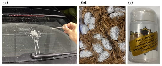
Figure 2.
Type of bird droppings (a) Fake poop, (b) owl droppings, (c) UGUISU.
1.3.3. Insects
Insects are refined materials used to express contamination of the sensor surface caused by insects that rush at the light during night driving. In fact, crickets used as insect food are available for purchase according to their size and type. In addition, unspecified flying insects exist, which can be collected outdoors. In this study, crickets were purchased for use in the insect field of the tests.
2. Research Equipment and Materials
2.1. Experimental Environment Configuration
Figure 3 shows the customized test equipment for this study. It consists of a fixed part that can fix sensors and window samples, a cleaning part that cleans with washers and air, a collector part that collects data from experiment results, and a controller part that can control experiments. In addition, a sink, an airflow pump, and a drain tank are installed. (Part name—manufacturer: nozzle—MiSUMi (511, Yeongdong-daero, Gangnam-gu, Seoul, Republic of Korea); vision camera—CREVIS (29-4, Gigok-ro, Giheung-gu, Yongin-si, Gyeonggi-do, Republic of Korea); compressor—Wabco (23, Cheongbuksandan-ro, Cheongbuk-eup, Pyeongtaek-si, Gyeonggi-do, Republic of Korea); SMPS—Mean Well; arm jig—MiSUMi; production—Soonho Technology (109, Wauan-gil, Bongdam-eup, Hwaseong-si, Gyeonggi-do, Republic of Korea)).
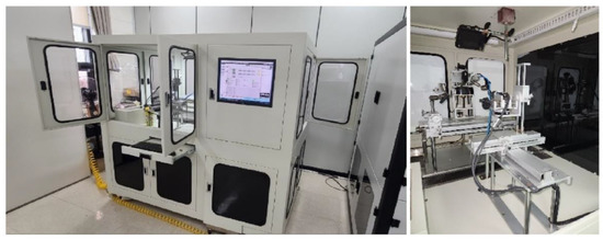
Figure 3.
Blockage performance evaluation device.
2.1.1. Fixed Part
In Figure 4a, the fixed part exhibits a shape in which the upper and lower parts are simultaneously engaged around the central point. The part in contact with the sample surface is made of urethane material to minimize damage and is designed to operate in all axial directions.
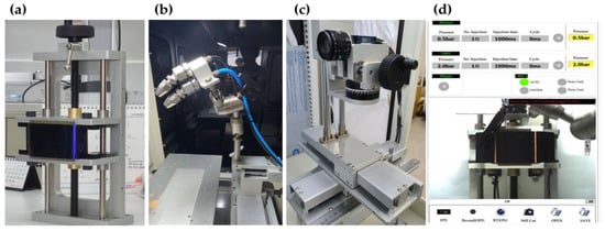
Figure 4.
(a) Sample fixed part, (b) cleaning part, (c) data collector part, and (d) controller part.
2.1.2. Cleaning Part
In Figure 4b, the cleaning part comprises two sets, with a washer nozzle and an air nozzle installed in each set. Fixed installation in all directions is possible by applying the fixed part as a joint. Moreover, the position and angle of the washer and air unit can be adjusted separately.
2.1.3. Collector Part
In Figure 4c, a camera capable of capturing high-definition images is installed in the collector part. Real-time videos and photographs can be acquired according to the settings. The file is automatically saved in the built-in server and is designed to operate in all axial directions.
2.1.4. Controller Part
The controller part is capable of remote-controlled real-time data storage and automatic control that sets and automatically executes the experiment sequence.
2.2. Blockage Reproduction Device
2.2.1. Dust Injector
The spray system (manufacturer: Spraysystem(45, Hambangmoe-ro 377beon-gil, Namdong-gu, Incheon, Republic of Korea), model name: AAB10000AUH) shown in Figure 5a enables the precise spraying of fluid through precise control of the spray nozzle. Most importantly, the spray controller can control the dust injection time, duty cycle, and quantitative dust injection. However, spraying a fluid with a concentration of less than 30% is recommended because dust with relatively large particles frequently clogs the nozzle.
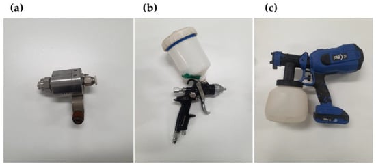
Figure 5.
(a) Spray system, (b) gravity spray gun, and (c) automatic injection gun.
The gravity spray device (manufacturer: Bluetech (100, Dalseong-ro, Jung-gu, Daegu, Republic of Korea), model name: H827) shown in Figure 5b can spray fluid using air pressure. The fluid container is located at the upper part of the spray gun to compensate for the problem of sedimentation of fluid (dust) during spraying. Therefore, it is advantageous in so far as it is feasible to evenly spray according to the ratio of the mixed fluid. Furthermore, it has the feature of evenly spraying fluid with relatively large particles. However, as it is a passive type, it cannot perform a constant quantity of spray on its own.
The automatic injection device (manufacturer: Prostormer (Level 2, Building 2, 169 Zhen Jiang Rd., Jiangbei district, Ningbo, Zhejiang, China), model name: PTHT264), shown in Figure 4c is a rechargeable electric sprayer, which has the advantage of being able to set the nozzle type, spray pattern, and spray angle to suit the user’s needs. However, it causes the phenomenon wherein the nozzle is clogged by dust with large particles.
In this study, the three injectors were tested with various fluids. The gravity spray gun was used, which does not cause clogging when spraying up to 50% concentration. The spray used an air pressure of 6 bar with a vertical distance of approximately 30 cm to the LiDAR window, which is the dust distribution target. The test for constant quantity spray was carried out at 3.5 g by measuring the weight of the sample before and after spraying with an electronic balance.
2.2.2. Insect Launcher
The insect gun (Figure 6a) was designed and manufactured in the form of a gun to improve mobility and accuracy (manufacturer: BMS TECH (1025-5, Gyeonggi-daero, Hwaseong-si, Gyeonggi-do, Republic of Korea)). The rate of firing can be adjusted using air pressure. In this study, as shown in Figure 6b, an air pressure of 6 bar was used at a distance of approximately 1 m in the vertical direction to the LiDAR window to simulate the impact of an oncoming insect while driving.
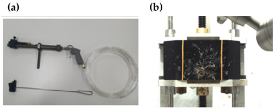
Figure 6.
(a) Insect air gun; (b) after insect impact.
2.3. Target LiDAR and Area Calculation S/W
2.3.1. Target LiDAR Sample
The selected target sample for this study, CARNAVICOM’s (13-25, Songdogwahak-ro 16beon-gil, Yeonsu-gu, Incheon, Republic of Korea) VL-R16 LiDAR window (Figure 7), includes a hard-coated window made of polycarbonate (PC) material and easily provides the blockage area unit spray amount and cleaning area.
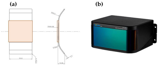
Figure 7.
(a) Window sample cover dimension; (b) target LiDAR (VL-R16).
2.3.2. Image Analyzer
As shown in Figure 8a,b, blockage tests were performed on an actual LiDAR—generating large variations in reception strength depending on the location of the blockage—the operating method of the LiDAR, and the location of the transmitter/receiver. As we focus on the blockage effect, a LiDAR sample cover was used for repeated investigations with identical conditions. In addition, the cleaning rate was determined considering the LiDAR sample cover’s area within the orange box, where the surface is free of any curves and is completely flat, as shown in Figure 7a. The concentration or area of the blockage covering the LiDAR cannot be manually analyzed because of its irregularity. Thus, automatic analysis software is essential. The cleaning surface area was calculated using Python as follows. An external light source was used to accentuate the contaminants on the LiDAR cover to capture an RGB image to the clearest extent possible. To reduce the effect of exposure to strong blue light on the clean cover, the blue value was subtracted from the RGB formula, as shown in Figure 8a,b. Although the blue value is included in the affected area, it is to a negligible degree, enabling the affected and clean areas to be distinguished. To quantify the leftover affected area, hue saturation lightness was used in place of RGB where L is the only unit used as the lightness value, as shown in Figure 8c. To identify the cleaning area on the actual LiDAR cover, various concentrations of blockage were sprayed onto the surface. Moreover, the signal strength was measured based on the LiDAR point cloud. Different blockage degrees were assigned to normal, thin, and thick blockages. As shown in Figure 8d, by comparing LiDAR point cloud values and images with blockage sprayed, we found values for the boundaries of the three areas.

Figure 8.
(a) LiDAR steady state: blue value = 53–58, (b) state of blue value = 0, (c) excluding reflected light, (d) RGB conversion.
2.4. Viscometer
The viscosity of blockage is significantly affected by the blockage type and concentration [38]. The viscosity of the main samples (ARI, JIS, KTD, KL, PT, FP) was measured to confirm the correlation between the blockage and the adhesion to the LiDAR window surface and the cleaning rate [38,39]. This was achieved by utilizing Brookfield’s DVE viscometer in Figure 9, which is a rotational measurement type.
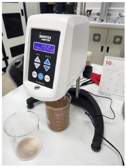
Figure 9.
DVE viscometer.
3. Experimental Conditions and Methods
3.1. Characteristics of Major Factors
3.1.1. Definition of Variables
For the performance comparison according to the blockage type and recipe, the manipulated variables consist of blockage type, water concentration, and dryness condition, as listed in Table 2. After spraying blockage, drying was performed for 5 min on all samples using a heating device (manufacturer: BOKUK, model name: BKH-1581PF, power: 1500 W). Because the spraying devices from different manufacturers use different washer pressure, air pressure, and duration, this study focused on blockage performance rather than setting specific pressure or duration values. To compare with cases where the blockage effect was lowered because the concentration was low, the washer pressure was 0.5 bar for 1 s of exposure and the air pressure was 2.0 bar for 1 s of exposure. The cleaning rate, which measures the blockage area remaining after washing, was selected as a dependent variable.

Table 2.
Main factors of the experiment.
3.1.2. Design of Experiment
The variables mentioned in Section 3.1.1 and the entire experimental progress checklist are shown in Table 3.

Table 3.
Experimental progress checklist.
3.2. Viscosity Analysis
The main equations required for calculating viscosity through the viscometer are as follows [40]: (The configuration of the viscometer is shown in Figure 10).
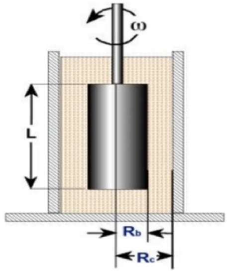
Figure 10.
Viscometer dimension.
As shown in Table 4, at low viscosity a 61 spindle was used, and 62 and 64 spindles were used at high viscosity. The viscosity was measured by applying the same spindle rotation speed of 60 rpm for all concentrations. The specifications of each spindle are shown in Table 4. Viscosity values were derived using the principle of viscometer operation.

Table 4.
Viscosity value measurement variable, spindle specification.
3.3. Methods of Experiment
3.3.1. Experimental Data Collection and Analysis Procedure
As seen in Figure 11, the blockage sample was applied to the LiDAR window. After acquiring a photograph before washing, the first and second washings were sequentially performed, and all data were saved as photographs. The cleaning rate was calculated by checking the remaining blockage area using an image analyzer. Figure 12 shows the process of using various types of blockage for the experiment.
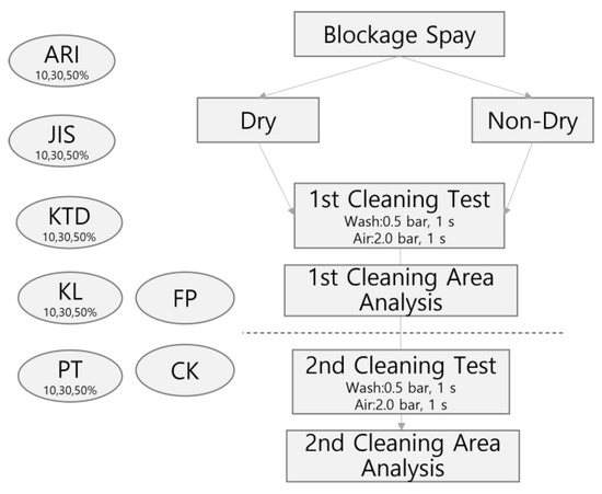
Figure 11.
Blockage test flow chart.
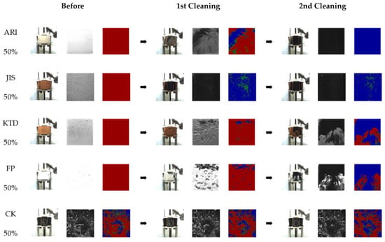
Figure 12.
Images of the experimental process according to the type of dust (ARI, JIS, KTD, FP, CK). Items are arranged in order according to the stages of before washing, first washing, and second washing. The image of each item is expressed using a real photo, black-and-white photo, and photo of the washing area expressed in RGB.
3.3.2. Repeat Test
In this study, 3.5 g of blockage was equally applied for each item and measurements were repeated three times. A similar trend was confirmed for the same samples. Furthermore, as a result of calculating the standard deviation and standard error to confirm the similarity of the three repeated tests, the average standard deviation of the repeated tests in all items was 2.03%, and the standard error was 1.43%, which mostly fell within the confidence range.
3.3.3. Data Validation Method
Figure 13 shows ANOVA, a method to verify the mean difference between groups. The assumptions of a single ANOVA include normality, equal variance, and independence. To compare the combined means of each level, checking whether the assumptions of the ANOVA are satisfied is necessary. Residual is the value subtracted from the appropriate fitted value in the model of the observed value that was actually tested. The residual plot is a graph that checks whether these assumptions are satisfied. This is a suitable model as there is no singularity in the data distribution, and normality assumption is met.
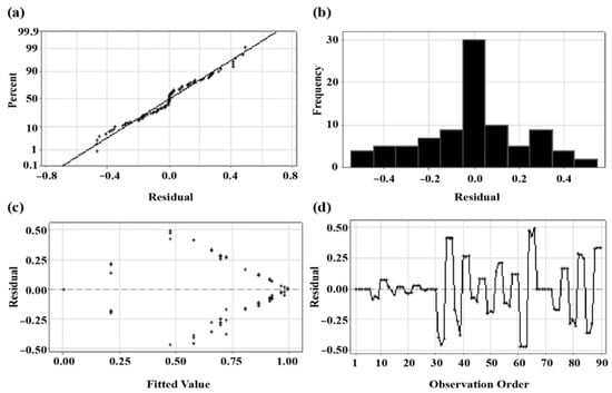
Figure 13.
(a) Normal probability plot, (b) histogram, (c) versus fits, and (d) versus order.
3.3.4. Random Forest
To demonstrate the importance of the factors used in the study on the cleaning rate, the random forest algorithm was applied to assign numerical values of statistical importance to each factor.
The random forest algorithm performance is mathematically represented by the IncNodePurity value that is calculated through a series of formulas. First, the Gini importance of each node of a single decision tree within the random forest is calculated:
where represents the parent node, represents the left child node, and represents the right child node. In addition, represents the number of samples, and represents the Gini impurity.
To calculate the Gini impurity, the following formula is used:
where represents the probability of data within the parent node classifying into the left child node, whereas represents the probability of data within the parent node classifying into the right child node.
Once all nodes are assigned their respective Gini importance values, the importance of each feature on a single decision tree can be calculated by
where represents the Gini importance of a specific feature on a singular node, whereas represents the Gini importance of all nodes.
Finally, as there are multiple decision trees associated with the random forest algorithm, the final feature importance, IncNodePurity, can be calculated as follows:
where represents the sum of the feature importance for each tree, and is the total number of trees used for the random forest algorithm.
Thus, the features with the highest value, or similarly the IncNodePurity, are classified so as to have higher overall importance as a feature in the random forest algorithm.
3.3.5. Two-Way ANOVA
The assumptions for two-way ANOVA are as follows:
- Normally distributed dependent values
- Independent samples
- Homogeneity of variances
The normality assumption can be tested by evaluating the QQ plot and conducting the Shapiro test, where a p-value > 0.05 confirms normality. Another important assumption that can overrule the normality assumption is the homogeneity of variances assumption, which can be made with Levene’s test. Obtaining a p-value greater than 0.05 confirms that the data exhibits equal variances. Though certain blockages are not normally distributed, all have equal variances; therefore, the Two-way ANOVA test can be conducted [41].
4. Result and Discussion
4.1. Importance Analysis of Major Factors Using Random Forest
Figure 14 shows that after conducting a test with 500 trees, it was determined that a random forest algorithm containing 50 trees would yield the smallest error. Thus, a random forest algorithm with 50 trees was used for the rest of the analysis discussed below.
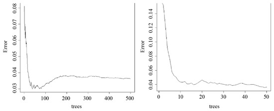
Figure 14.
Random forest algorithm (tree case 500, 50).
Figure 15 shows an example of a possible singular decision tree of the 50 decision trees used to develop the random forest algorithm.
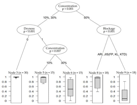
Figure 15.
Random forest tree case.
From the random forest algorithm feature importance results, Table 5 shows that blockage is the most important feature with an IncNodePurity value of 3.2143. This is followed by concentration and dryness with IncNodePurity values of 2.5226 and 1.9834, respectively. The mean of squared errors is relatively low at approximately 0.0468, with a percent variance above 72%. In conclusion, Figure 16 confirms that the random forest algorithm can confidently provide the first cleaning rate using only these three variables, with blockage being the most important feature.

Table 5.
Evaluation of the factor importance of the random forest model.
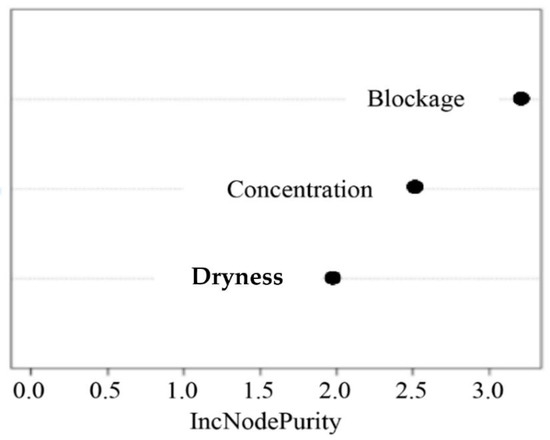
Figure 16.
Variable importance.
4.2. Analysis of the Effects of Concentration and Dryness Conditions according to the Blockage Factors
Based on the results of Section 4.1, among the three factors, blockage, concentration, and dryness, the impact analysis on concentration and dryness was conducted based on the blockage factor, which is the most important factor in the cleaning rate. The two-way ANOVA technique was used to facilitate the analysis of two factors—concentration and dryness.
4.2.1. ARI (Arizona Dust A2 Fine)
In Figure 17, according to the QQ plot, certain observations deviate significantly from the rest of the data, whereas the Shapiro–Wilk normality test rules the dataset as non-normal (p < 0.05), agreeing with the observations from the QQ plot. However, Table 6 reveals that the homogeneity of variance assumption is met, as Levene’s test for homogeneity of variance results show a p-value (0.0616) greater than 0.05. Thus, the two-way ANOVA test can be performed on this dataset.
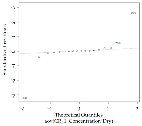
Figure 17.
ARI normal QQ plot.

Table 6.
Shapiro and Levene’s test result (ARI).
In Table 7, from the two-way ANOVA test results for the ARI dataset, all p-values for concentration, dryness, and the interaction between concentration and dryness are below 0.05. This implies that concentration and dryness as well as their interaction term are significant factors for determining the cleaning rate. In addition, TukeyHSD results show a significant difference between all concentration groups’ differences in cleaning rate, barring the 10–30% difference (p = 0.1761). A significant difference in cleaning rates for ARI under non-dry conditions with 10% and 30% could not be observed.

Table 7.
Summary of factor importance and Tukey HSD results (ARI).
4.2.2. JIS (Class 8)
According to the QQ plot in Figure 18, certain observations deviate significantly from the rest of the data, whereas the Shapiro–Wilk normality test rules the dataset as non-normal (p < 0.05), agreeing with the observations from the QQ plot. However, the homogeneity of variance assumption is met as the Levene’s test for homogeneity of variance results show a p-value (0.3061) greater than 0.05 (shown in Table 8). Thus, the two-way ANOVA test can be performed on this dataset.
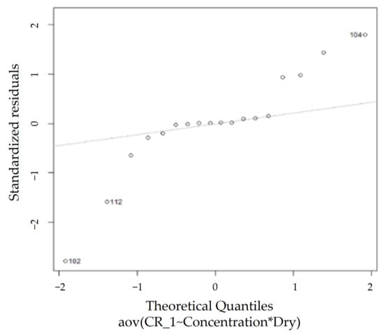
Figure 18.
JIS normal QQ plot.

Table 8.
Shapiro and Levene’s test result (JIS).
From the two-way ANOVA test results for the JIS dataset in Table 9, all p-values for concentration, dryness, and the interaction between concentration and dryness are below 0.05. This implies that concentration and dryness as well as their interaction term are significant factors for determining the cleaning rate. In addition, TukeyHSD results exhibit a significant difference between all concentration groups’ differences in the cleaning rate, barring a 10–30% difference (p = 0.2833). JIS, similar to ARI, shows an insignificant difference in the cleaning rate between non-dry conditions at 10% and 30% concentration levels.

Table 9.
Summary of factor importance and Tukey HSD results (JIS).
4.2.3. KTD
According to the QQ plot in Figure 19, certain observations that deviate significantly from the rest of the data are observed, whereas the Shapiro–Wilk normality test rules the dataset as non-normal (p < 0.05), agreeing with the observations from the QQ plot. However, the homogeneity of variance assumption is met, as the Levene’s test for homogeneity of variance results exhibits a p-value (0.1975) greater than 0.05, as shown in Table 10. Thus, conducting the two-way ANOVA test on this dataset is feasible.
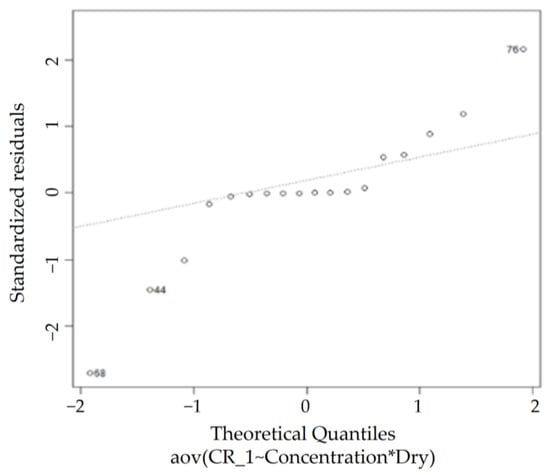
Figure 19.
KTD normal QQ plot.

Table 10.
Shapiro and Levene’s test result (KTD).
From the two-way ANOVA test results for the KTD dataset in Table 11, all p-values for concentration, dryness, and the interaction between concentration and dryness are below 0.05. This implies that concentration and dryness as well as their interaction terms are significant factors for determining the cleaning rate. In addition, TukeyHSD results show a significant difference between all concentration groups’ differences (p < 0.05) in the cleaning rate.

Table 11.
Summary of factor importance and Tukey HSD results (KTD).
4.2.4. KL (Kaolin)
According to the QQ plot in Figure 20, certain observations that deviate significantly from the rest of the data are observed, whereas the Shapiro–Wilk normality test rules the dataset as non-normal (p < 0.05), agreeing with the observations from the QQ plot. However, the homogeneity of variance assumption is met, as the Levene’s test for homogeneity of variance results show a p-value (0.1324) greater than 0.05, as shown in Table 12. Thus, performing a two-way ANOVA test on this dataset is feasible.
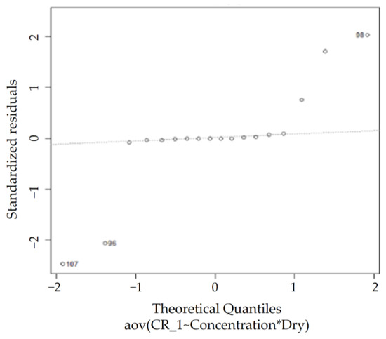
Figure 20.
KL normal QQ plot.

Table 12.
Shapiro and Levene’s test result (KL).
From the two-way ANOVA test results for the KL dataset in Table 13, all p-values for concentration, dryness, and the interaction between concentration and dryness are below 0.05. This implies that concentration and dryness as well as their interaction term are significant factors for determining the cleaning rate. In addition, Tukey HSD results exhibit a significant difference between all concentration groups’ differences (p < 0.05) in the cleaning rate.

Table 13.
Summary of factor importance and Tukey HSD results (KL).
4.2.5. Portland Cement (PT)
According to the QQ plot and the Shapiro–Wilk normality test in Figure 21, the data are observed to be normal (p > 0.05). In addition, the homogeneity of variance assumption is also met, as the Levene’s test for homogeneity of variance results show a p-value (0.6425) greater than 0.05, as shown in Table 14. Thus, performing the two-way ANOVA test on this dataset is feasible.
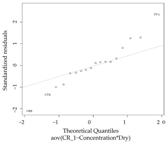
Figure 21.
PT normal QQ plot.

Table 14.
Shapiro and Levene’s test result (PT).
From the two-way ANOVA test results for the PT dataset in Table 15, all p-values for concentration, dryness, and the interaction between concentration and dryness are below 0.05. This implies that concentration and dryness as well as their interaction term are significant factors for determining the cleaning rate. In addition, Tukey HSD results show a significant difference between all concentration groups’ differences (p < 0.05) in the cleaning rate.

Table 15.
Summary of factor importance and Tukey HSD results (PT).
4.3. Comparison of Cleaning Rates according to Blockage, Concentration, and Dryness Conditions
Figure 22a shows the cleaning rate with respect to concentration for all blockage factors under dry conditions. The characteristics of each blockage were apparent, and various trends in the cleaning rate change according to the concentration of each blockage factor were revealed. JIS and PT showed negligible changes in the cleaning rate by concentration, and ARI showed an apparent change in the cleaning rate in all concentration ranges. Particularly for KTD and KL, the change in concentration was considerably large, from 10% to 30%, and the change in the cleaning rate from 30% to 50% concentration was relatively small at 13.89% for KTD and 0.14% for KL. This is because the cleaning condition, which is an independent variable of this experimental condition, is insufficient. The FT and CK values, which are comparative indicators, fall within the 30% and 10% ranges of KTD, respectively. In the future, when considering the influence of bird droppings or insects, equivalent performance is expected within the 30–50% concentration range of KTD. Finally, the cleaning rate of KL was exceedingly low at concentrations above 30%; thus, comparison with other factors is irrelevant.
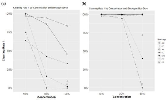
Figure 22.
(a) Blockage and concentration cleaning rate result graph (dry), (b) blockage and concentration cleaning rate result graph (non-dry).
Figure 22b shows the cleaning rate by concentration for all blockage factors under non-drying conditions. All cleaning rates were high compared with dry conditions. In the range of 10–30%, all blockage cleaning rates showed high values of 94.53% or more. However, ARI, JIS, and PT did not affect the concentration change, and only KTD and KL showed a sharp decrease in the cleaning rate in the 50% range. KL did not exhibit clear characteristics under the cleaning conditions used in this study at 50% concentration, even under non-dry conditions. Thus, KL exhibited a higher performance as a blockage than other factors, and accurate distinction is difficult when employing the fixed washing performance in this study.
The overall performance was verified based on the above results. Compared with the performances of FP and CK, which are comparative indicators, blockages with appropriate performance can be created by utilizing the cleaning rate result according to the concentrations of KTD and PT depending on dry or non-dry conditions.
Figure 23 compares the dry and non-dry characteristics of each blockage factor. Regardless of whether the environment was dry, ARI, JIS, and KTD demonstrated a cleaning rate >96.52% at 10% concentration. However, most of the dry and non-dry cleaning rates clearly differed at 30% concentration. In the cases of KTD, KL, and PT, a noticeable variation in the cleaning rate was observed. Furthermore, concentration and drying circumstances impact these results because the cleaning rate, which ranges from 10% to 30% under comparatively non-dry conditions, is marginally changed. Because the cleaning rate immediately dropped to almost zero in a non-dry state at a concentration of 50%, KL could not validate the drying characteristics. According to FP, a significant difference of 62.47% in the cleaning rate between dry and non-dry conditions was noted.
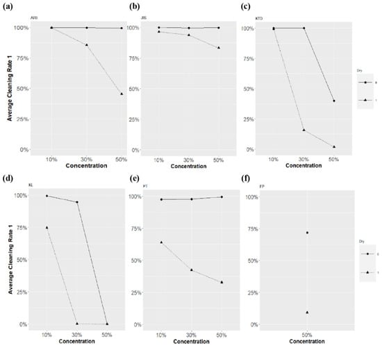
Figure 23.
Comparison of dry and non-dry characteristics of blockages (a) ARI, (b) JIS, (c) KTD, (d) KL, (e) PT, (f) FP.
4.4. Comparison of Characteristics according to Cleaning Cycles
This study compared the performance according to the blockage type, concentration, and dryness condition based on the constant cleaning performance. However, the following graph compares the cleaning rate results under two repetitions of the same cleaning performance, as discussed below.
In the comparison of the difference between the first and second cleaning rates in Figure 24, most factors with a large difference arose from a concentration of 30% or more. Only KL and PT were affected at 10% concentration. Various results can be obtained from the graph, depending on the washing performance (e.g., amount of water, spray pressure, time). In particular, the cleaning rate increased rapidly when KTD, PT, and FP at 50% concentration and KTD, KL, and PT at 30% concentration were washed twice.
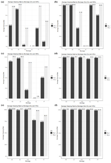
Figure 24.
Difference between first and second cleaning rates. (a) Concentration 50%, first cleaning rate; (b) 50%, second cleaning rate; (c) 30%, first cleaning rate; (d) 30%, second cleaning rate; (e) 10%, first cleaning rate; and (f) 10%, second cleaning rate.
4.5. Correlation between Viscosity and Cleaning Rate
To identify the correlation between viscosity and cleaning rate and to compare the viscosity and cleaning rate values, the viscosity values were measured using a viscometer for each blockage and concentration, as shown in Table 16.

Table 16.
Viscosity result for each blockage (Unit: mPa·s).
The correlation between the viscosity and cleaning rate was analyzed. The closer the correlation is to zero, the weaker the connection between the viscosity and cleaning rate. A negative value was obtained when the viscosity and cleaning rate were high and low, respectively. Conversely, a positive value was obtained when both the cleaning rate and viscosity were high.
The negative correlation coefficient in the dry state indicates that the viscosity and cleaning rate are inversely correlated, as shown in Table 17. In particular, the correlation tendency was clearly confirmed at 30 and 50% concentrations under dry conditions. However, under the dry condition of 10% and the non-dry condition of 10 and 30%, the cleaning rate by blockage factor is mostly high at 90% or more; thus, the correlation tendency is unclear. Therefore, the correlation with viscosity is not large because the correlation coefficient with viscosity is close to 0. Although the results were not satisfactory under all conditions, Figure 25 shows that the correlation between viscosity and cleaning rate was high under dry conditions, and a large correlation was observed only at 50% concentration under non-dry conditions. If the viscosity is high, cleaning is difficult because the blockage strongly adheres to the LiDAR window sample. Moreover, this adhesion can be effective in selecting suitable parameters for spray testing. KTD and KL are efficient for cleaning tests because a large amount of dust can adhere to a small amount of the target sample.

Table 17.
Correlation between cleaning rate and viscosity.

Figure 25.
Viscosity versus cleaning rate comparison graph. (a) Concentration 10%; (b) concentration 30%; and (c) concentration 50%.
5. Conclusions
Based on the cleaning rate, this study examined how various factors, such as the blockage type, concentration, additive, and dryness, which are the main factors in the evaluation of the cleaning performance of autonomous driving sensors, affect blockage performance. The findings of this study can be applied to various blockages, and blockages with the desired performance, such as bird droppings and insects, can be implemented by adjusting the dryness and concentration.
KTD dust, representing the Korean environment, was presented, and the cleaning rate was compared in addition to ARI and JIS. At a concentration of 30% or higher, KTD exhibited a considerably lower cleaning rate than ARI and JIS. The effect of KTD as a substitute dust was similar to that of bird droppings as the cleaning rate for KTD was within the range similar to that of the cleaning rate for bird droppings. Experimental tools and techniques for performance testing were proposed in this study to compare the performance of dust in a particular region in the future. Therefore, it will be possible to increase the variety of dust options, lower the price of dust purchases, and represent the actual environment as closely as possible.
To evaluate the sensor cleaning performance for the safe autonomous driving of SAE level four or higher, experiments can be conducted under various conditions by using various recipes (e.g., type, concentration, drying) suggested in this study. Furthermore, they can also be used for various sensor cleaning evaluations by utilizing methods such as cross-mixing and the five blockages covered in this study, even in severe cases, such as bird droppings and insects, which are frequently encountered during actual road driving.
Finally, the number of washings had a substantial effect on the cleaning rate. Further research is required to optimize the cleaning technology through a comparative test of the cleaning rate for blockages, such as KTD, KL, FP, and CK, under severe conditions with the cleaning conditions, such as water and air injection pressure and time, fixed to a low specification as in this study and used as independent variables. Furthermore, the blockage effect on camera and radar sensors and LiDAR sensors and the optimal cleaning conditions for each sensor need to be researched. This method can be used for LiDAR, which is the target sensor of this study, and also cameras, radars, and ultrasonic sensors. It can be widely used in various tests involving devices such as automobile windshields, mirrors, and license plates.
Author Contributions
Conceptualization, S.S.; methodology, S.S. and W.L.; software, H.J.; formal analysis, S.S.; data curation, M.L.; writing—original draft preparation, S.S.; writing—review and editing, H.-C.R. and J.J.; supervision, C.K., H.L. and S.C.; project administration, J.L.; validation, H.-C.R.; All authors have read and agreed to the published version of the manuscript.
Funding
This work is supported by the Korea Agency for Infrastructure Technology Advancement (KAIA) grant funded by the Ministry of Land, Infrastructure and Transport (Project No. RS-2021_KA162419).
Institutional Review Board Statement
Not applicable.
Informed Consent Statement
Not applicable.
Data Availability Statement
Not applicable.
Conflicts of Interest
The authors declare no conflict of interest.
References
- Trierweiler, M.; Caldelas, P.; Gröninger, G.; Peterseim, T.; Neumann, C. Influence of sensor blockage on automotive LiDAR systems. In Proceedings of the 2019 IEEE SENSORS, Montreal, QC, Canada, 27–30 October 2019; pp. 1–4. [Google Scholar] [CrossRef]
- Santo, B. ICVS Intelligent Automotive Industry Alliance 2022. Sensor Cleaning Is a Nightmare for ADAS, ADAS Sensors Create a Cleaning Nightmare—EE Times. Available online: https://www.eetimes.com/adas-sensors-create-a-cleaning-nightmare/ (accessed on 10 January 2023).
- Linkov, J. The Race to Protect Car Sensors from Their Biggest Foes: Dirt and Weather. Consumer Reports. Available online: https://www.consumerreports.org/car-maintenance/protect-car-sensors-from-dirt-and-weather/ (accessed on 10 January 2023).
- Bluestar. The Importance of Windshield Wipers & Washers. Available online: https://www.bluestar.com/get_informed/article/the-importance-of-windshield-wipers-washers (accessed on 10 January 2023).
- Pozo-Antonio, J.S.; Puente, I.; Pereira, M.F.C.; Rocha, C.S.A. Quantification and mapping of deterioration patterns on granite surfaces by means of mobile LiDAR data. Measurement 2019, 140, 227–236. [Google Scholar] [CrossRef]
- Liu, B.; Zhang, S.; He, J. Deformation measurement of glass structure using FBG sensor. Photonic Sens. 2019, 9, 367–375. [Google Scholar] [CrossRef]
- Rivero, J.R.V.; Tahiraj, I.; Schubert, O.; Glassl, C.; Buschardt, B.; Berk, M.; Chen, J. Characterization and simulation of the effect of road dirt on the performance of a laser scanner. In Proceedings of the 2017 IEEE 20th International Conference on Intelligent Transportation, Yokohama, Japan, 16–19 October 2017. [Google Scholar] [CrossRef]
- Vikas, N.R.; Pahwa, G.; Mohanty, S. Camera Blockage Detection in Autonomous Driving using Deep Neural Networks. In Proceedings of the 2022 Second International Conference on Computer Science, Engineering and Applications (ICCSEA), Gunupur, India, 8 September 2022; pp. 1–6. [Google Scholar] [CrossRef]
- Persistence Market Research, Automotive Sensor Cleaning System Market, 2020 Persistence Market Research, PMR Analysis, New York City, USA, 2020. pp. 87–91. Available online: https://www.persistencemarketresearch.com/market-research/automotive-sensor-cleaning-system-market.asp (accessed on 7 December 2020).
- Jung, U.; Choi, S.-S. Classification and characterization of tire-road wear particles in road dust by density. Polymers 2022, 14, 1005. [Google Scholar] [CrossRef] [PubMed]
- Dong, Q.; Huang, Z.; Li, W.; Li, Z.; Song, X.; Liu, W.; Wang, T.; Bi, J.; Shi, J. Polarization LiDAR measurements of dust optical properties at the junction of the taklimakan Desert–Tibetan Plateau. Remote Sens. 2022, 14, 558. [Google Scholar] [CrossRef]
- Wang, Y.T.; Peng, C.C.; Ravankar, A.A.; Ravankar, A. A single LiDAR-based feature fusion indoor localization algorithm. Sensors 2018, 18, 1294. [Google Scholar] [CrossRef] [PubMed]
- Linnhoff, C.; Rosenberger, P.; Winner, H. Refining object-based LiDAR sensor modeling—Challenging ray tracing as the magic bullet. IEEE Sens. J. 2021, 21, 24238–24245. [Google Scholar] [CrossRef]
- Vierhub-Lorenz, V.; Kellner, M.; Zipfel, O.; Reiterer, A. A Study on the effect of multispectral LiDAR data on automated semantic segmentation of 3D-point clouds. Remote Sens. 2022, 14, 6349. [Google Scholar] [CrossRef]
- Liu, H.; Yu, Y.; Song, W.; Jiang, Q.; Pang, F.; Wang, T. Spectrally flat supercontinuum generation in a ZBLAN fiber pumped by erbium-doped mode-locked fiber laser. Photonic Sens. 2019, 9, 302–308. [Google Scholar] [CrossRef]
- Jung, H.J.; Lee, I.H. Performance analysis of millimeter-wave UAV swarm networks under blockage effects. Sensors 2020, 20, 4593. [Google Scholar] [CrossRef]
- Jeon, H.; Kim, Y.; Choi, M.; Park, D.; Son, S.; Lee, J.; Choi, G.; Lim, Y. CARLA simulator-based evaluation framework development of lane detection accuracy performance under sensor blockage caused by heavy rain for autonomous vehicle. IEEE Robot. Autom. Lett. 2022, 7, 9977–9984. [Google Scholar] [CrossRef]
- Jokela, M.; Kutila, M.; Pyykönen, P. Testing and validation of automotive point-cloud sensors in adverse weather conditions. Appl. Sci. 2019, 9, 2341. [Google Scholar] [CrossRef]
- Fersch, T.; Buhmann, A.; Koelpin, A.; Weigel, R. The influence of rain on small aperture LiDAR sensors. In Proceedings of the 2016 German Microwave Conference (GeMiC), Bochum, Germany, 14–16 March 2016; pp. 84–87. [Google Scholar] [CrossRef]
- Hasirlioglu, S.; Doric, I.; Lauerer, C.; Brandmeier, T. Modeling and simulation of rain for the test of automotive sensor systems. In Proceedings of the 2016 IEEE Intelligent Vehicles Symposium (IV), Gothenburg, Sweden, 19–22 June 2016; pp. 286–291. [Google Scholar] [CrossRef]
- Hasirlioglu, S.; Kamann, A.; Doric, I.; Brandmeier, T. Test methodology for rain influence on automotive surround sensors. In Proceedings of the 2016 IEEE 19th International Conference on Intelligent Transportation Systems (ITSC), Rio de Janeiro, Brazil, 1–4 November 2016; pp. 2242–2247. [Google Scholar] [CrossRef]
- Goodin, C.; Carruth, D.; Doude, M.; Hudson, C. Predicting the influence of rain on LiDAR in ADAS. Electronics 2019, 8, 89. [Google Scholar] [CrossRef]
- Filgueira, A.; Gonzalez-Jorge, H.; Laǵuela, S.; íazVilarino, L.D.; Arias, P. Quantifying the influence of rain in LiDAR performance. Measurement 2017, 95, 143–148. [Google Scholar] [CrossRef]
- Rasshofer, R.H.; Spies, M.; Spies, H. Influences of weather phenomena on automotive laser radar systems. Adv. Radio Sci. 2011, 9, 49–60. [Google Scholar] [CrossRef]
- Mohammadi, A.; Rahmati, M.; Malik, H. Location-aware beamforming for MIMO-enabled UAV communications: An unknown input observer approach. IEEE Sens. J. 2011, 22, 8206–8215. [Google Scholar] [CrossRef]
- Ren, R.; Fu, H.; Xue, H.; Sun, Z.; Ding, K.; Wang, P. Towards a fully automated 3D reconstruction system based on LiDAR and GNSS in challenging scenarios. Remote Sens. 2021, 13, 1981. [Google Scholar] [CrossRef]
- Wang, Q.; Yan, C.; Tan, R.; Feng, Y.; Sun, Y.; Liu, Y. 3D-CALI: Automatic calibration for camera and LiDAR using 3D checkerboard. Measurement 2022, 203, 111971. [Google Scholar] [CrossRef]
- Trierweiler, M.; Peterseim, T.; Neumann, C. Automotive LiDAR pollution detection system based on total internal reflection techniques. In Light-Emitting Devices, Materials, and Applications XXIV; International Society for Optics and Photonics: Bellingham, WA, USA, 2020; p. 1130216. [Google Scholar]
- Zhang, H.; Wagner, F.; Saathoff, H.; Vogel, H.; Hoshyaripour, C.; Bachmann, V.; Förstner, J.; Leisner, T. Comparison of scanning LiDAR with other remote sensing measurements and transport model predictions for a Saharan dust case. Remote Sens. 2022, 14, 1693. [Google Scholar] [CrossRef]
- Montanaro, A.; Allocca, L.; Maccariello, G.; Frosina, E.; Romagnuolo, L.; Senatore, A. Experimental analysis of a water spray for the sensors cleaning at different injection pressures. In Proceedings of the 2021 IEEE International Workshop on Metrology for Automotive (MetroAutomotive), Bologna, Italy, 1–2 July 2021; pp. 121–124. [Google Scholar] [CrossRef]
- Göktürk, K.; Jönsson, A. Developing a Resource-Efficient Sensor Cleaning System for Autonomous Heavy Vehicles. Master’ Thesis, KTH, Stockholm, Sweden, 2019. [Google Scholar]
- dlhBOWLES Camera & Sensor Wash Systems, HD. Available online: https://www.youtube.com/watch?v=Z1nhbyyGCQI (accessed on 4 February 2019).
- Ficosa Camera Cleaning. Available online: https://www.ficosa.com/products/underhood/sensor-and-camera-cleaning/ (accessed on 4 February 2019).
- Clean Sensors Regardless of Weather Conditions Thanks to New Valeo Solution. 2019. Available online: https://valeo.prowly.com/67657-clean-sensors-regardless-of-weather-conditions-thanks-to-new-valeo-solution-everview-lidar/ (accessed on 13 August 2019).
- Continental Automotive-Washer Systems. Camera Cleaning Systems. 2019. Available online: https://www.continental-automotive.com/en-gl/Passenger-Cars/Safety/Products/Washer-Systems (accessed on 23 July 2021).
- ISO 12103-1:2016-03; Road Vehicles—Test Contaminants for Filter Evaluation—Part 1: Arizona Test Dust. Beuth: Berlin, Germany, 2016.
- Waymo’s Self-Driving Car Has a Delightful Way to Clean Bird Poop off Its Sensors. 2019. Available online: http://digg.com/2017/waymo-clean-lidar (accessed on 27 June 2019).
- Pradhan, M.; Johir, A.B.H.; Kandasamy, J.; Ratnaweera, H.; Vigneswaran, S. Effects of Viscosity on Submerged Membrane Microfiltration Systems. Membranes 2022, 12, 780. [Google Scholar] [CrossRef]
- Dereli, R.K.; Grelot, A.; Heffernan, B.; van der Zee, F.P.; van Lier, J.B. Implications of changes in solids retention time on long term evolution of sludge filterability in anaerobic membrane bioreactors treating high strength industrial wastewater. Water Res. 2014, 59, 11–22. [Google Scholar] [CrossRef]
- Barnes, W.J.P. Data Analysis. In More Solutions to Sticky Problems, 2nd ed.; Commerce Blvd.: Middleborough, MA, USA, 2017; pp. 21–22. [Google Scholar]
- Keselman, H.J.; Huberty, C.J.; Lix, L.M.; Olejnik, S.; Cribbie, R.A.; Donahue, B.; Kowalchuk, R.K.; Lowman, L.L.; Petoskey, M.D.; Keselman, J.C.; et al. Statistical practices of educational researchers: An analysis of their ANOVA, MANOVA, and ANCOVA analyses. Rev. Educ. Res. 1998, 68, 350–386. [Google Scholar] [CrossRef]
Disclaimer/Publisher’s Note: The statements, opinions and data contained in all publications are solely those of the individual author(s) and contributor(s) and not of MDPI and/or the editor(s). MDPI and/or the editor(s) disclaim responsibility for any injury to people or property resulting from any ideas, methods, instructions or products referred to in the content. |
© 2023 by the authors. Licensee MDPI, Basel, Switzerland. This article is an open access article distributed under the terms and conditions of the Creative Commons Attribution (CC BY) license (https://creativecommons.org/licenses/by/4.0/).


