

Deep Learning-Empowered Digital Twin Using Acoustic Signal for Welding Quality Inspection
Abstract
1. Introduction
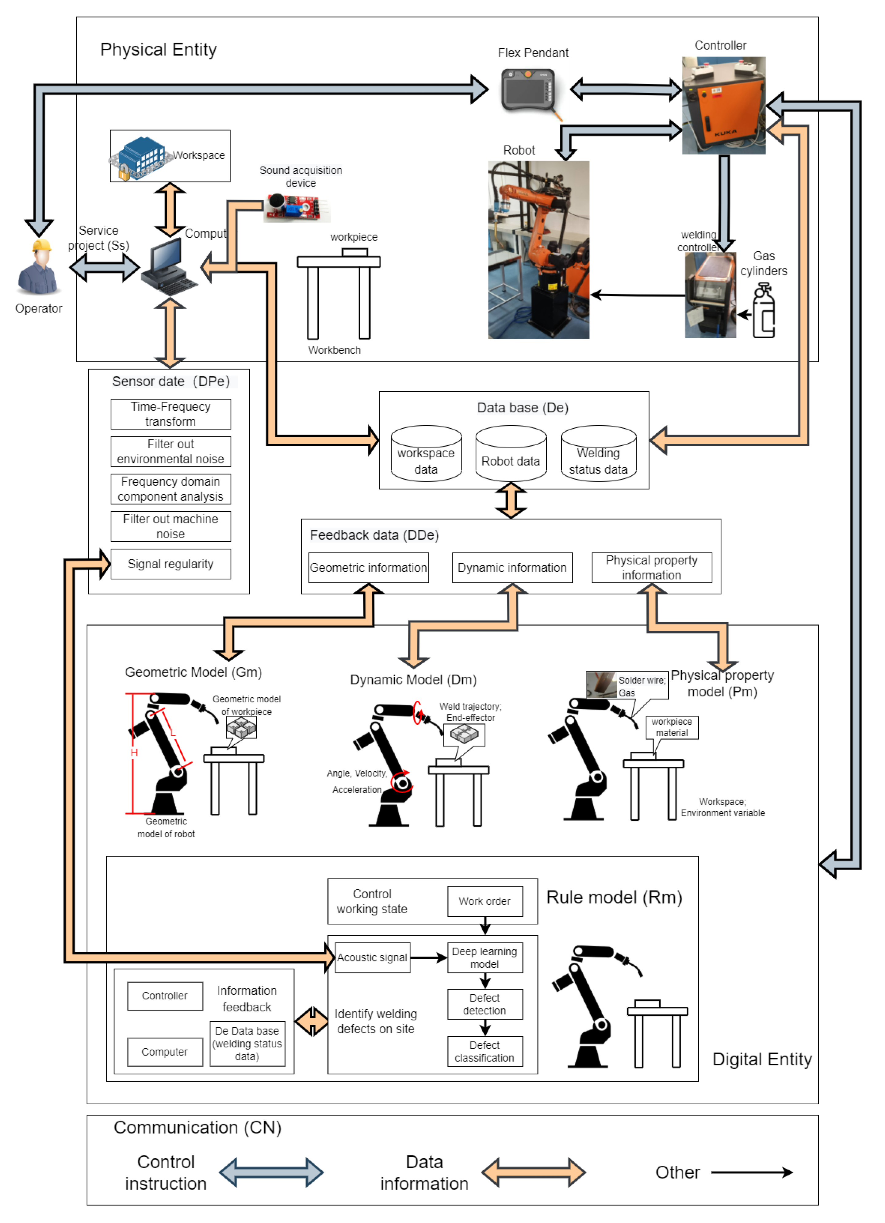
2. Digital Twin System
2.1. Digital Twin of Industrial Robot
2.1.1. Physical Entity
2.1.2. Digital Entity
2.1.3. Service Project
2.1.4. Data
2.1.5. Communication
2.2. Building a DT
3. Signal Preprocessing
3.1. Acoustic Signal Analysis
3.2. Improved Wavelet Denoising
4. Identification and Classification
4.1. Classification Model
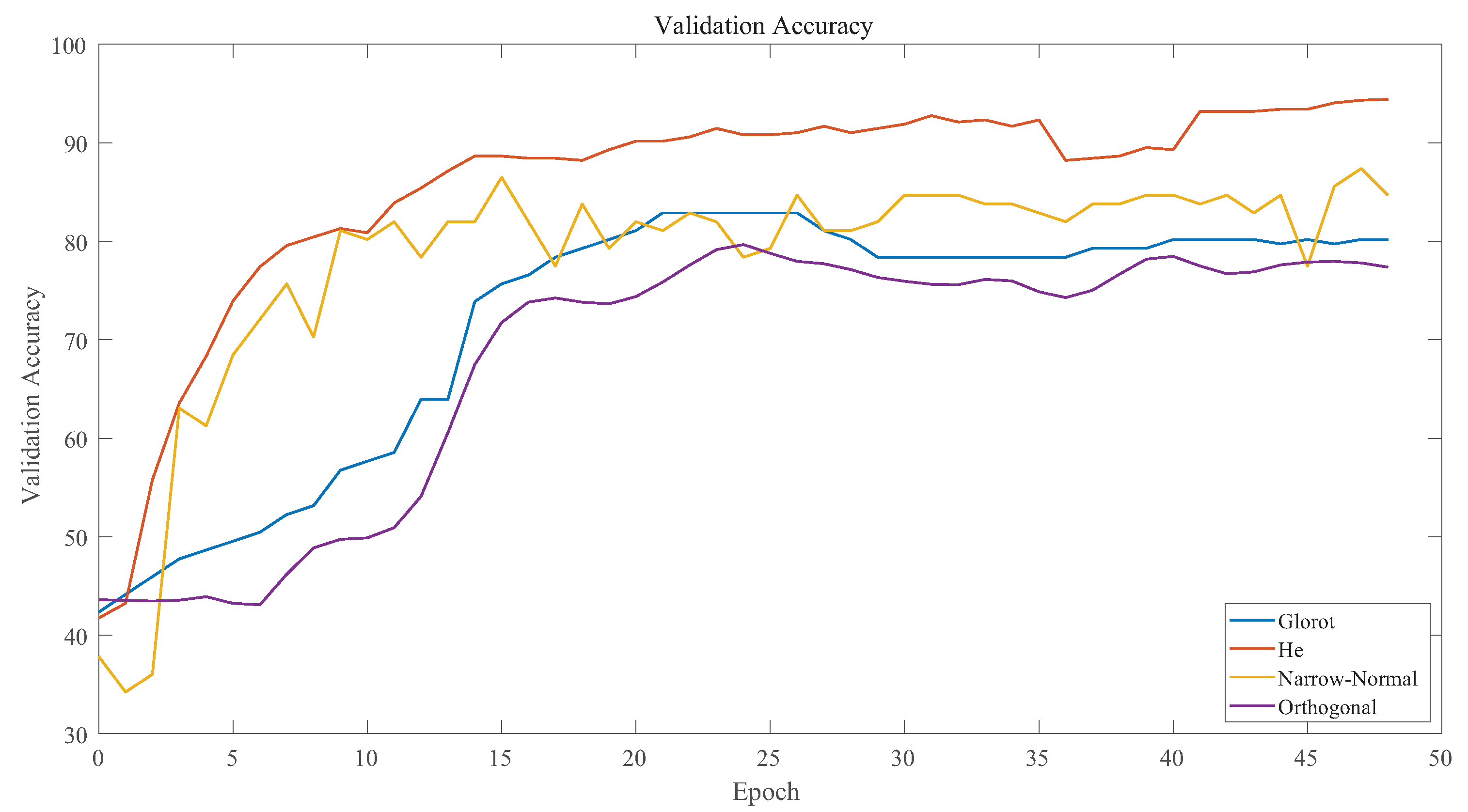
4.2. Model Training and Parameters
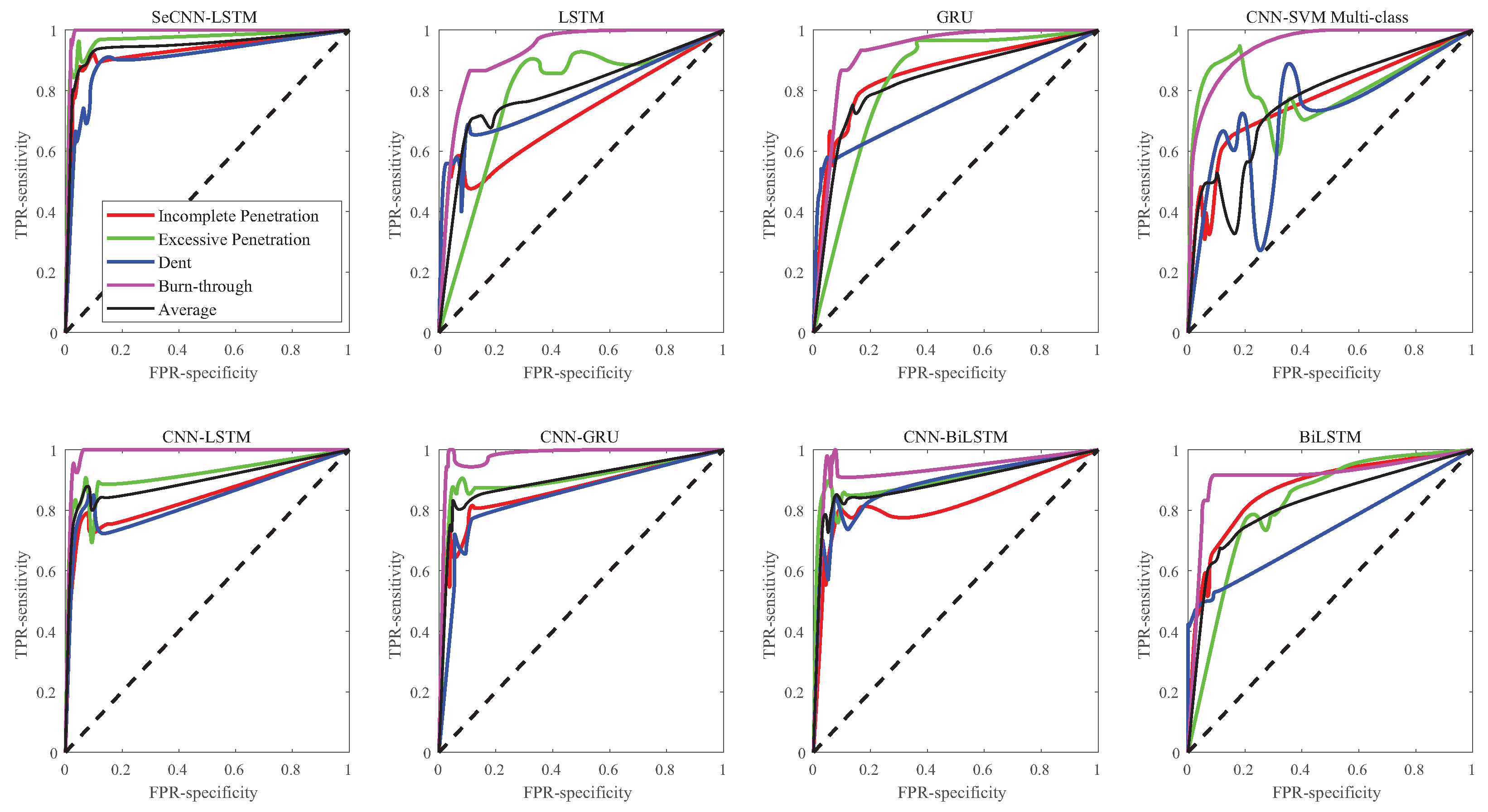
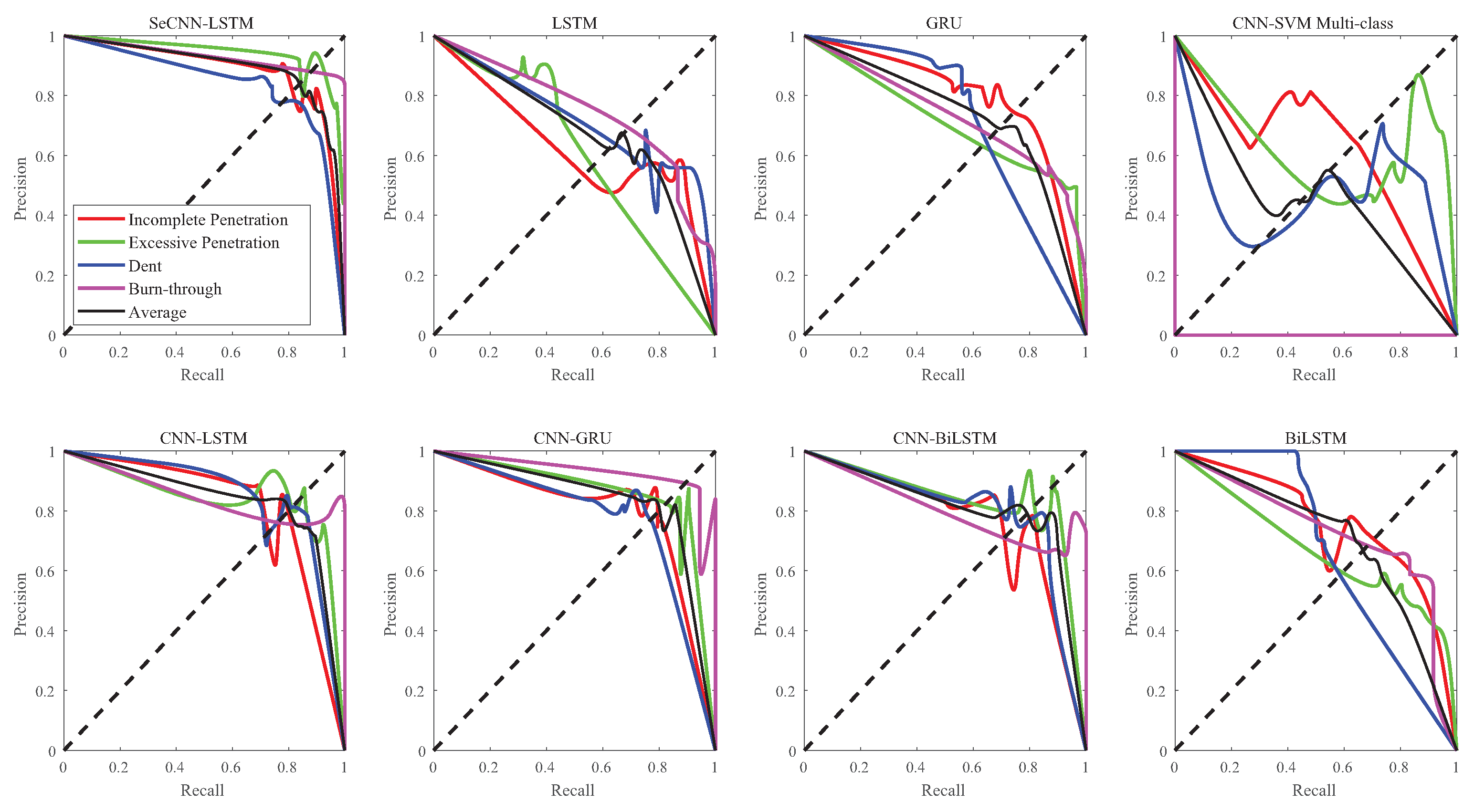
4.3. Model Comparison
5. Conclusions
Author Contributions
Funding
Institutional Review Board Statement
Informed Consent Statement
Data Availability Statement
Conflicts of Interest
References
- Zhang, Z.; Wen, G.; Chen, S. On-Line Monitoring and Defects Detection of Robotic Arc Welding: A Review and Future Challenges. In Transactions on Intelligent Welding Manufacturing; Springer: Berlin/Heidelberg, Germany, 2019; pp. 3–28. [Google Scholar] [CrossRef]
- Xu, J.; Chen, S. The Review of Spectrum Detection and Ultrasonic Vibration Control of Porosity Defects in Aluminum Alloy Welding. In Transactions on Intelligent Welding Manufacturing; Springer: Berlin/Heidelberg, Germany, 2020; pp. 3–24. [Google Scholar] [CrossRef]
- Cui, Y.; Shi, Y.; Zhu, T.; Cui, S. Welding penetration recognition based on arc sound and electrical signals in K-TIG welding. Measurement 2020, 163, 107966. [Google Scholar] [CrossRef]
- Chen, S.B.; Lv, N. Research evolution on intelligentized technologies for arc welding process. J. Manuf. Process. 2014, 16, 109–122. [Google Scholar] [CrossRef]
- Ma, G.; Yuan, H.; Yu, L.; He, Y. Monitoring of weld defects of visual sensing assisted GMAW process with galvanized steel. Mater. Manuf. Process. 2021, 36, 1178–1188. [Google Scholar] [CrossRef]
- Zhang, Z.; Wen, G.; Chen, S. Weld image deep learning-based on-line defects detection using convolutional neural networks for Al alloy in robotic arc welding. J. Manuf. Process. 2019, 45, 208–216. [Google Scholar] [CrossRef]
- Cao, Y.; Wang, Z.; Hu, S.; Wang, W. Modeling of weld penetration control system in GMAW-P using NARMAX methods. J. Manuf. Process. 2021, 65, 512–524. [Google Scholar] [CrossRef]
- Bonikila, P.R.; Indimath, S.S.; Shajan, N. Failure assessment of Mash Seam Weld breakage and development of online weld inspection system for early detection of weld failure. Eng. Fail. Anal. 2022, 133, 105967. [Google Scholar] [CrossRef]
- Horvat, J.; Prezelj, J.; Polajnar, I.; Čudina, M. Monitoring Gas Metal Arc Welding Process by Using Audible Sound Signal. Stroj. Vestnik– J. Mech. Eng. 2011, 2011, 267–278. [Google Scholar] [CrossRef]
- Gao, Y.; Zhao, J.; Wang, Q.; Xiao, J.; Zhang, H. Weld bead penetration identification based on human-welder subjective assessment on welding arc sound. Measurement 2020, 154, 107475. [Google Scholar] [CrossRef]
- Lv, N.; Xu, Y.; Li, S.; Yu, X.; Chen, S. Automated control of welding penetration based on audio sensing technology. J. Mater. Process. Technol. 2017, 250, 81–98. [Google Scholar] [CrossRef]
- Liu, L.; Chen, H.; Chen, S. Quality analysis of CMT lap welding based on welding electronic parameters and welding sound. J. Manuf. Process. 2022, 74, 1–13. [Google Scholar] [CrossRef]
- Na, L.; Chen, S.j.; Chen, Q.h.; Tao, W.; Zhao, H.; Chen, S.b. Dynamic welding process monitoring based on microphone array technology. J. Manuf. Process. 2021, 64, 481–492. [Google Scholar] [CrossRef]
- Wang, Q.; Gao, Y.; Huang, L.; Gong, Y.; Xiao, J. Weld bead penetration state recognition in GMAW process based on a central auditory perception model. Measurement 2019, 147, 106901. [Google Scholar] [CrossRef]
- Boschert, S.; Rosen, R. Digital Twin—The Simulation Aspect. In Mechatronic Futures; Springer: Berlin/Heidelberg, Germany, 2016; Book Section Chapter 5; pp. 59–74. [Google Scholar] [CrossRef]
- Tao, F. Make more digital twins. Nature 2019, 573, 490–491. [Google Scholar] [CrossRef] [PubMed]
- Qi, Q.; Tao, F.; Hu, T.; Anwer, N.; Liu, A.; Wei, Y.; Wang, L.; Nee, A.Y.C. Enabling technologies and tools for digital twin. J. Manuf. Syst. 2021, 58, 3–21. [Google Scholar] [CrossRef]
- Cimino, C.; Negri, E.; Fumagalli, L. Review of digital twin applications in manufacturing. Comput. Ind. 2019, 113, 103130. [Google Scholar] [CrossRef]
- Lu, Y.; Liu, C.; Wang, K.I.K.; Huang, H.; Xu, X. Digital Twin-driven smart manufacturing: Connotation, reference model, applications and research issues. Robot. Comput.-Integr. Manuf. 2020, 61, 101837. [Google Scholar] [CrossRef]
- Ren, S.; Ma, Y.; Ma, N.; Chen, Q.; Wu, H. Digital twin for the transient temperature prediction during coaxial one-side resistance spot welding of Al5052/CFRP. J. Manuf. Sci. Eng. 2022, 144, 031015. [Google Scholar] [CrossRef]
- Xu, W.; Cui, J.; Li, L.; Yao, B.; Tian, S.; Zhou, Z. Digital twin-based industrial cloud robotics: Framework, control approach and implementation. J. Manuf. Syst. 2021, 58, 196–209. [Google Scholar] [CrossRef]
- Zhuang, C.; Miao, T.; Liu, J.; Xiong, H. The connotation of digital twin, and the construction and application method of shop-floor digital twin. Robot. Comput.-Integr. Manuf. 2021, 68, 102075. [Google Scholar] [CrossRef]
- Wang, Q.; Jiao, W.; Zhang, Y. Deep learning-empowered digital twin for visualized weld joint growth monitoring and penetration control. J. Manuf. Syst. 2020, 57, 429–439. [Google Scholar] [CrossRef]
- Tipary, B.; Erdős, G. Generic development methodology for flexible robotic pick-and-place workcells based on Digital Twin. Robot. Comput.-Integr. Manuf. 2021, 71, 102140. [Google Scholar] [CrossRef]
- Tao, F.; Zhang, M.; Liu, Y.; Nee, A.Y.C. Digital twin driven prognostics and health management for complex equipment. CIRP Ann. 2018, 67, 169–172. [Google Scholar] [CrossRef]
- Imran, M.S.; Rahman, A.F.; Tanvir, S.; Kadir, H.H.; Iqbal, J.; Mostakim, M. An analysis of audio classification techniques using deep learning architectures. In Proceedings of the 2021 6th International Conference on Inventive Computation Technologies (ICICT), Coimbatore, India, 20–22 January 2021; pp. 805–812. [Google Scholar]
- Tran, V.T.; Tsai, W.H. Acoustic-Based Train Arrival Detection Using Convolutional Neural Networks with Attention. IEEE Access 2022, 10, 72120–72131. [Google Scholar] [CrossRef]
- Boulmaiz, A.; Messadeg, D.; Doghmane, N.; Taleb-Ahmed, A. Design and implementation of a robust acoustic recognition system for waterbird species using TMS320C6713 DSK. Int. J. Ambient Comput. Intell. (IJACI) 2017, 8, 98–118. [Google Scholar] [CrossRef]
- Maria, A.; Jeyaseelan, A.S. Development of optimal feature selection and deep learning toward hungry stomach detection using audio signals. J. Control Autom. Electr. Syst. 2021, 32, 853–874. [Google Scholar] [CrossRef]
- Saddam, S.A.W. Wind Sounds Classification Using Different Audio Feature Extraction Techniques. Informatica 2022, 45. [Google Scholar] [CrossRef]


| Name/Brand | Material | |
|---|---|---|
| Workpiece | Stainless steel S30400 | , , , , , 17.5–19.5, 8–10.5 |
| Solder Wire | ER70s-6 | , , 1.4–1.85, , , |
| Shielding Gas | CO2 |
| Samle 1 | Sample 2 | Sample 3 | |
|---|---|---|---|
| Soft shreshold | 3.6525 | 6.5828 | 12.2800 |
| Hart shreshold | 3.5645 | 6.3638 | 12.1649 |
| Improved shreshold | 4.1886 | 6.9739 | 12.3590 |
| Accuracy | Precision | Recall | |||||||
|---|---|---|---|---|---|---|---|---|---|
| Incomplete Penetration | Excessive Pentration | Dent | Burn-Through | Incomplete Penetration | Excessive Pentration | Dent | Burn-Through | ||
| SeCNN-LSTM | 90.99% | 93.93% | 92.59% | 90% | 85.71% | 88.57% | 89.28% | 90% | 100% |
| LSTM | 63.96% | 93.3% | 47.3% | 93.8% | 64% | 38.9% | 86.7% | 53.6% | 94.1% |
| GRU | 61.26% | 67.9% | 61.9% | 85.7% | 66.87% | 59.4% | 83.9% | 42.9% | 90 % |
| CNN-SVM | 83.78% | 71.4% | 92.3% | 73.1% | 0% | 74.1% | 88.9% | 70.4% | 0% |
| CNN-LSTM | 73.87% | 89.3% | 73.5% | 68.6% | 92.9% | 61% | 96.2% | 88.9% | 76.5% |
| CNN-GRU | 74.77% | 72.7% | 83.8% | 83.3% | 75% | 88.9% | 91.2% | 50% | 81.8% |
| CNN-BiLSTM | 79.28% | 64.7% | 84.4% | 88.9% | 72.2% | 81.5% | 84.4% | 63.2% | 92.9% |
| BiLSTM | 68.47% | 86.7% | 58.8% | 78.3% | 68.2% | 39.4% | 90.9% | 62.1% | 93.8% |
| Incomplete Penetration | Excessive Pentration | Dent | Burn-Through | Average | |
|---|---|---|---|---|---|
| SeCNN-LSTM | 0.9274 | 0.9687 | 0.9052 | 0.9895 | 0.9443 |
| LSTM | 0.7172 | 0.7827 | 0.7809 | 0.9279 | 0.7952 |
| GRU | 0.8573 | 0.8343 | 0.7664 | 0.9269 | 0.8320 |
| CNN-SVM | 0.7687 | 0.8188 | 0.7241 | 0.9470 | 0.7634 |
| CNN-LSTM | 0.8426 | 0.9159 | 0.8353 | 0.9868 | 0.8951 |
| CNN-GRU | 0.8641 | 0.9012 | 0.8448 | 0.9795 | 0.8965 |
| CNN-BiLSTM | 0.8238 | 0.9016 | 0.8842 | 0.9310 | 0.8872 |
| BiLSTM | 0.8695 | 0.8203 | 0.7346 | 0.9097 | 0.8210 |
| Incomplete Penetration | Excessive Pentration | Dent | Burn-Through | Average | |
|---|---|---|---|---|---|
| SeCNN-LSTM | 0.8838 | 0.9428 | 0.8391 | 0.9322 | 0.8938 |
| LSTM | 0.6256 | 0.5991 | 0.7160 | 0.7461 | 0.6719 |
| GRU | 0.7900 | 0.7061 | 0.7103 | 0.7323 | 0.7303 |
| CNN-SVM | 0.6125 | 0.6317 | 0.4665 | 0 | 0.4501 |
| CNN-LSTM | 0.8154 | 0.8401 | 0.8479 | 0.8492 | 0.8323 |
| CNN-GRU | 0.7955 | 0.8612 | 0.7763 | 0.9329 | 0.8358 |
| CNN-BiLSTM | 0.7696 | 0.8338 | 0.7951 | 0.8070 | 0.8061 |
| BiLSTM | 0.7546 | 0.6678 | 0.6683 | 0.7284 | 0.7018 |
| Incomplete Penetration | Excessive Pentration | Dent | Burn-Through | Average | |
|---|---|---|---|---|---|
| SeCNN-LSTM | 0.7406 | 0.7741 | 0.6984 | 0.7561 | 0.7436 |
| LSTM | 0.5628 | 0.4454 | 0.5911 | 0.5414 | 0.5716 |
| GRU | 0.6345 | 0.5556 | 0.5857 | 0.5672 | 0.6212 |
| CNN-SVM | 0.5023 | 0.6321 | 0.5384 | 0 | 0.3984 |
| CNN-LSTM | 0.6818 | 0.7488 | 0.7166 | 0.7199 | 0.7212 |
| CNN-GRU | 0.6945 | 0.7573 | 0.6685 | 0.7871 | 0.7296 |
| CNN-BiLSTM | 0.6441 | 0.7720 | 0.6766 | 0.7387 | 0.7127 |
| BiLSTM | 0.5652 | 0.5488 | 0.5325 | 0.5631 | 0.5792 |
Disclaimer/Publisher’s Note: The statements, opinions and data contained in all publications are solely those of the individual author(s) and contributor(s) and not of MDPI and/or the editor(s). MDPI and/or the editor(s) disclaim responsibility for any injury to people or property resulting from any ideas, methods, instructions or products referred to in the content. |
© 2023 by the authors. Licensee MDPI, Basel, Switzerland. This article is an open access article distributed under the terms and conditions of the Creative Commons Attribution (CC BY) license (https://creativecommons.org/licenses/by/4.0/).
Share and Cite
Ji, T.; Mohamad Nor, N. Deep Learning-Empowered Digital Twin Using Acoustic Signal for Welding Quality Inspection. Sensors 2023, 23, 2643. https://doi.org/10.3390/s23052643
Ji T, Mohamad Nor N. Deep Learning-Empowered Digital Twin Using Acoustic Signal for Welding Quality Inspection. Sensors. 2023; 23(5):2643. https://doi.org/10.3390/s23052643
Chicago/Turabian StyleJi, Tao, and Norzalilah Mohamad Nor. 2023. "Deep Learning-Empowered Digital Twin Using Acoustic Signal for Welding Quality Inspection" Sensors 23, no. 5: 2643. https://doi.org/10.3390/s23052643
APA StyleJi, T., & Mohamad Nor, N. (2023). Deep Learning-Empowered Digital Twin Using Acoustic Signal for Welding Quality Inspection. Sensors, 23(5), 2643. https://doi.org/10.3390/s23052643