


Thermal Calibration of Triaxial Accelerometer for Tilt Measurement


Abstract
:1. Introduction
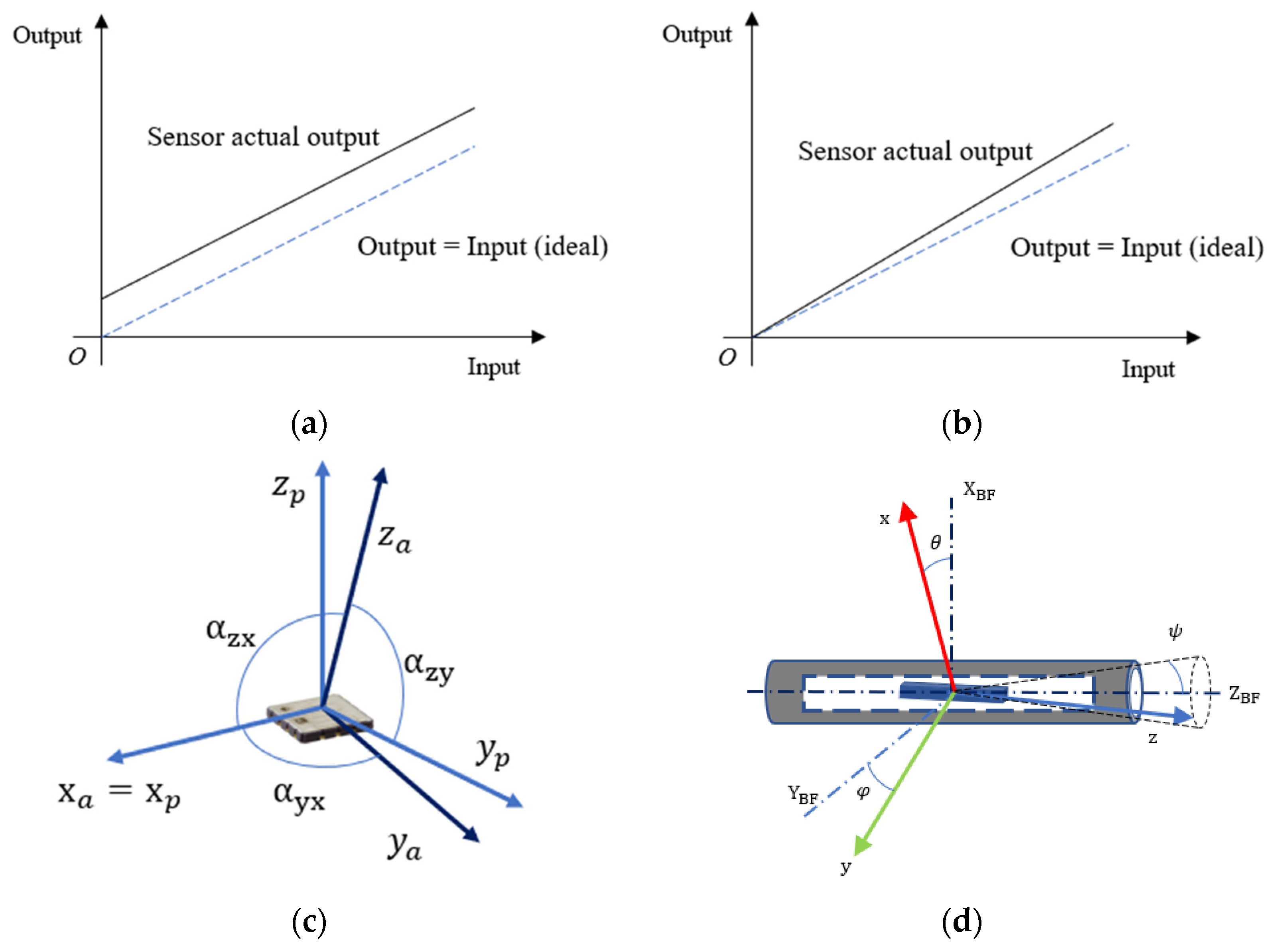
2. Error Source and Error Model
2.1. Sensor Frame Error Model
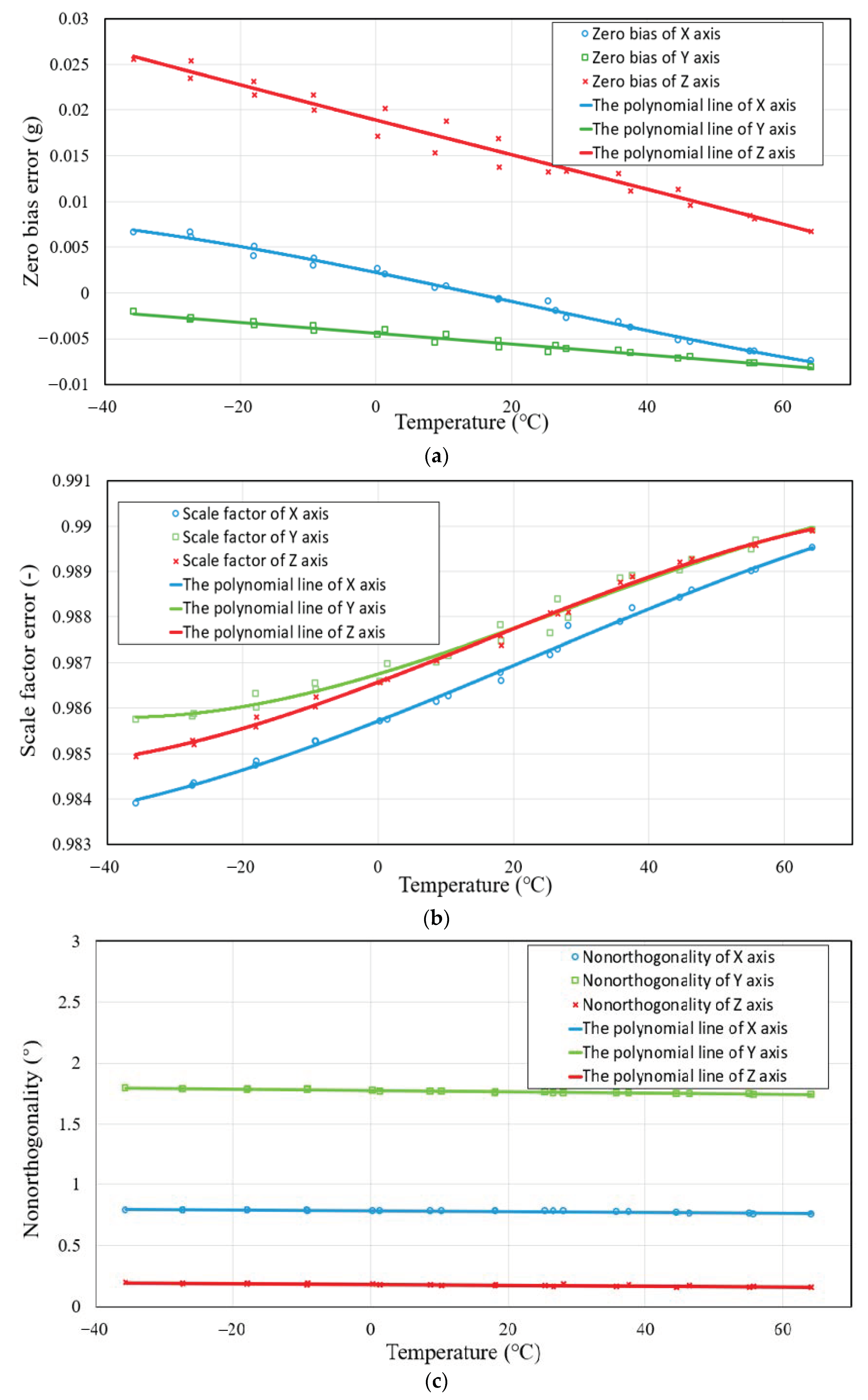
2.2. Temperature Dependence
- (1)
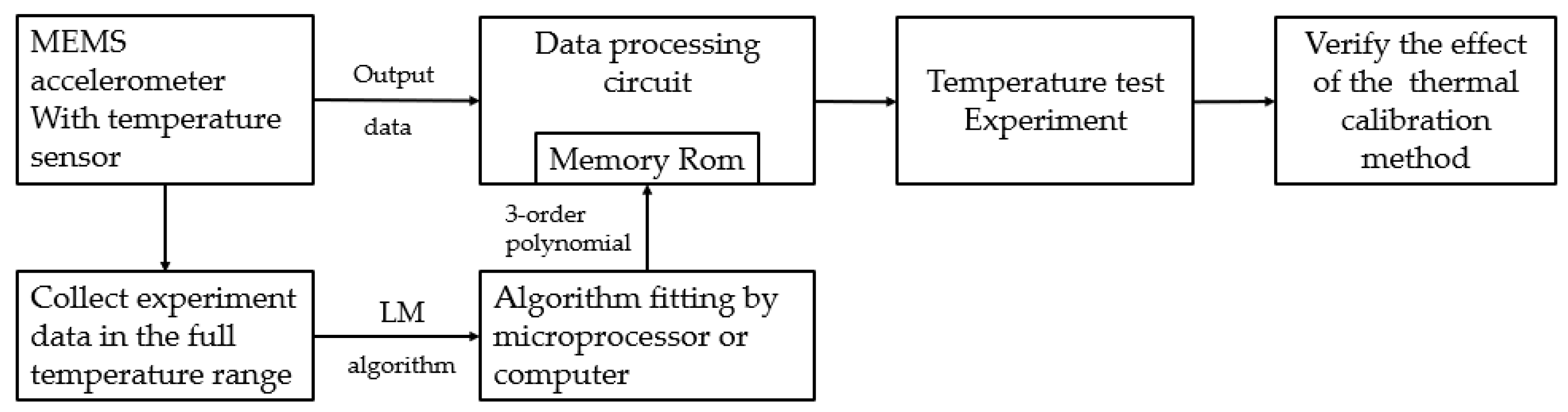
- Temperature calibration: developing accurate and reliable thermal models of the sensor errors, i.e., establishing a relationship between the sensor errors and the sensor temperature;
- (2)
- Temperature compensation: compensating the thermal drift of the sensor errors based on their temperature during the accelerometer’s operation process. Both of these processes are dependent on the temperature generated by the accelerometer’s internal temperature sensors.
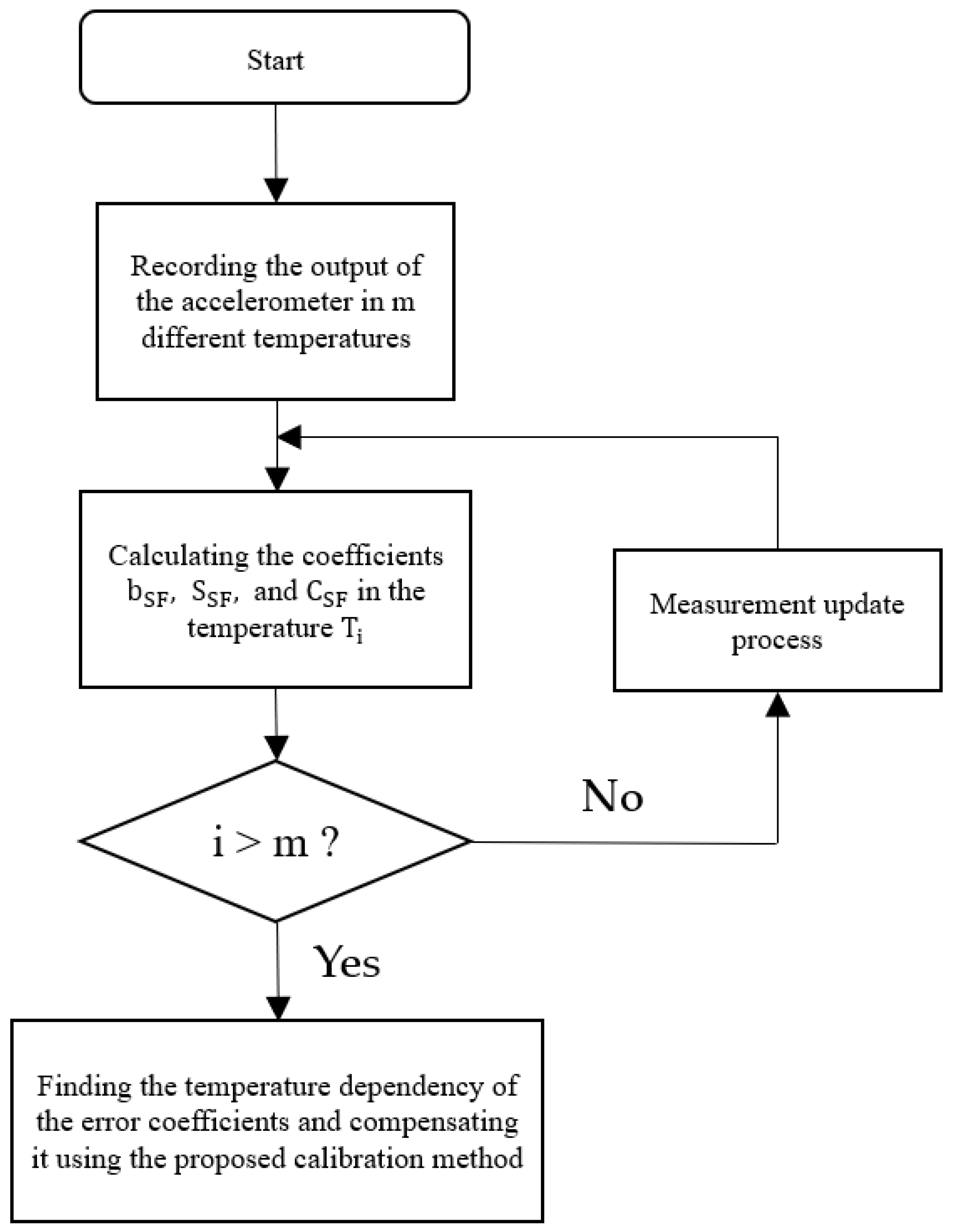
3. Calibration Method
3.1. Levenberg-Marquardt Algorithm
- (1)
- The Gradient Descent Method: The Gradient Descent (GD) algorithm is a commonly used minimization method that updates the parameter values in the opposite direction of the gradient from the objective function. The GD algorithm is highly convergent and can be used for optimization problems with thousands of parameters. The GD algorithm update that modifies the in the direction of the steepest descent can be defined as shown in Equation (5).where is a positive scalar corresponding to the step in the steepest-descent direction; is a Jacobian matrix based on the vector ; can be set as the inverse matrix of the measurement error covariance matrix.
- (2)
- The Gauss-Newton Method: The Gauss-Newton method is a method for the minimization of the sum-of-squares target function. For medium-sized problems, the Gauss-Newton method usually converges faster than the gradient descent method. The formula for the GN algorithm to reduce is given by the following Equation (6).where indicates the GN algorithm update of the parameter estimated to lead to the minimization of .
- (3)
- The Levenberg-Marquardt method: The Levenberg-Marquardt algorithm adaptively changes the parameter updates between gradient descent parameter iterations and Gauss-Newton parameter iterations to achieve optimal progress in the minimization of The LM algorithm can be described by Equation (7).where is the Jacobian matrix of vectors is the weighting diagonal matrix; is adaptively weighted to reach optimal progress in minimization. The damping factor is adjusted at each iteration.
3.2. Least-Squares Fitting of Data by Polynomials
4. Experiments and Results
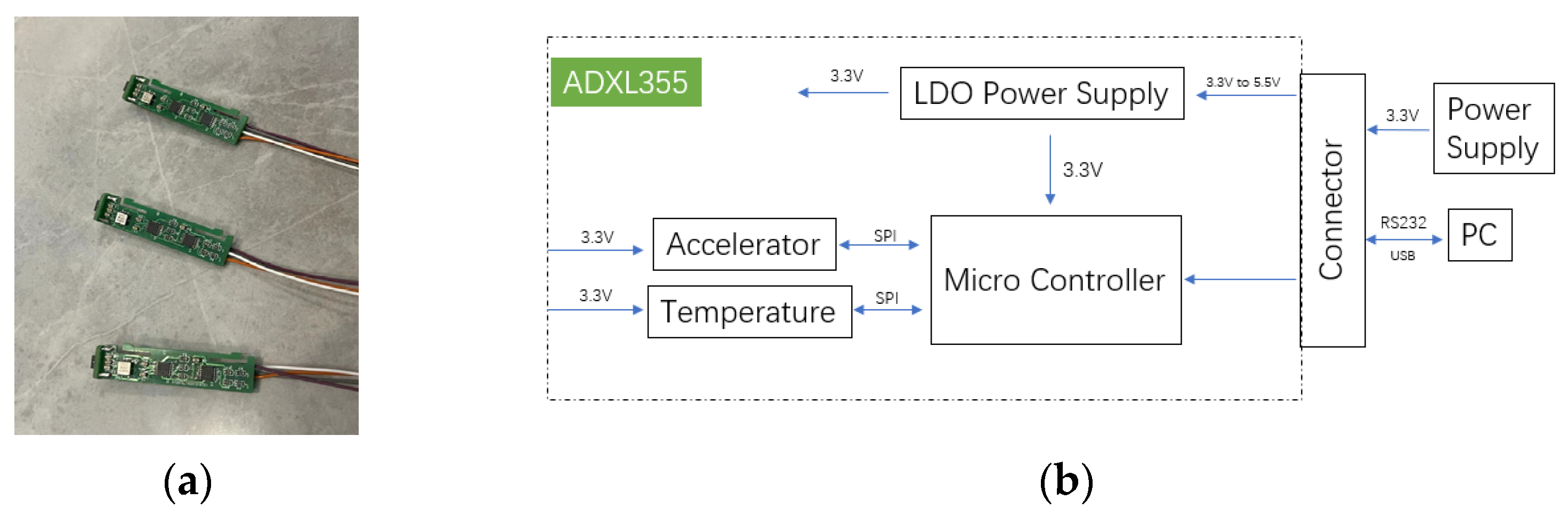
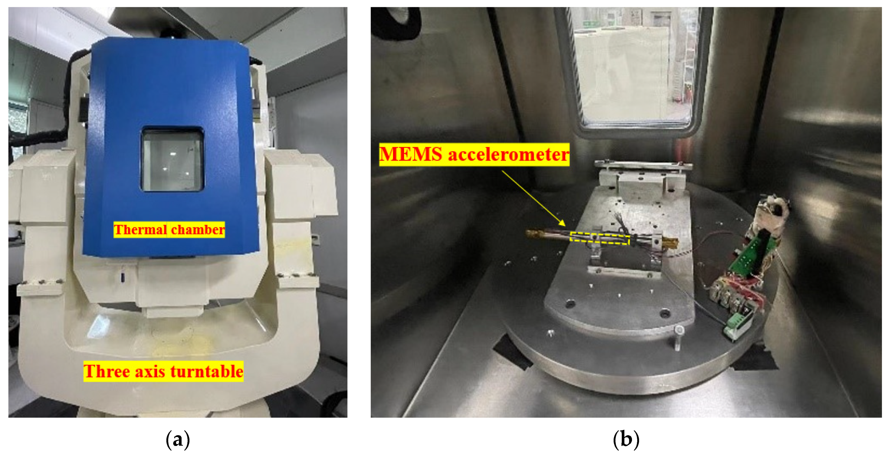
4.1. Calibrated Sensors and Measurement Setup
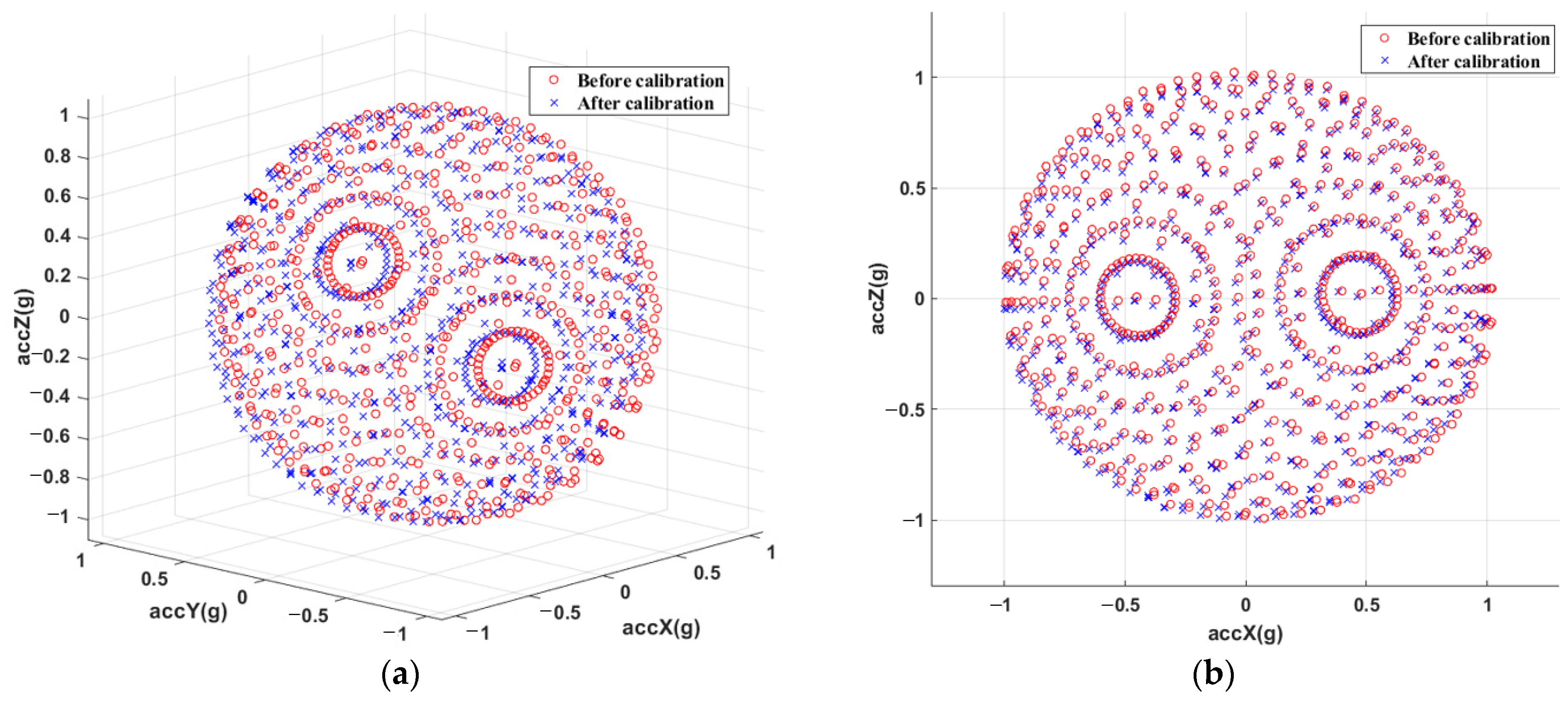
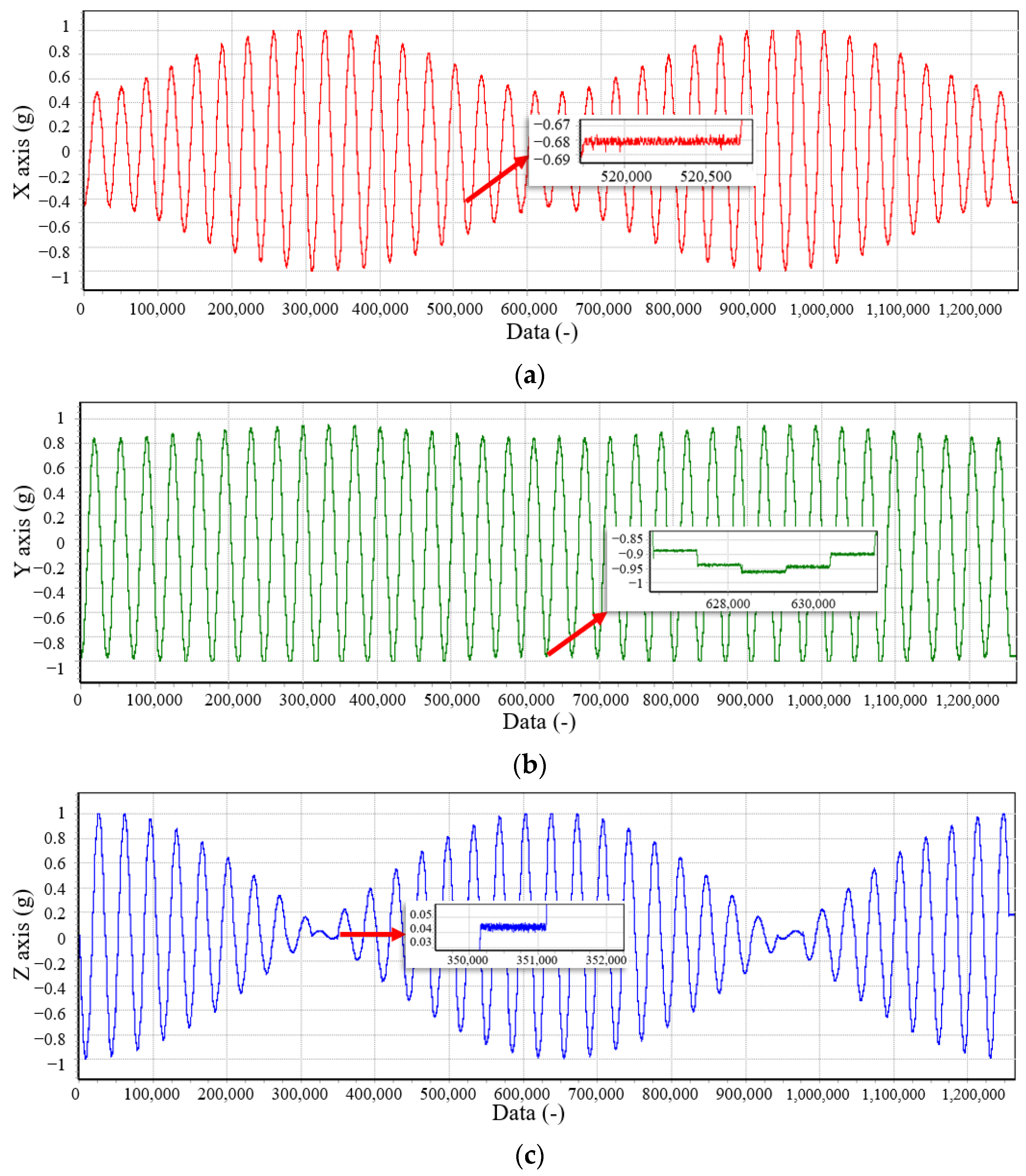
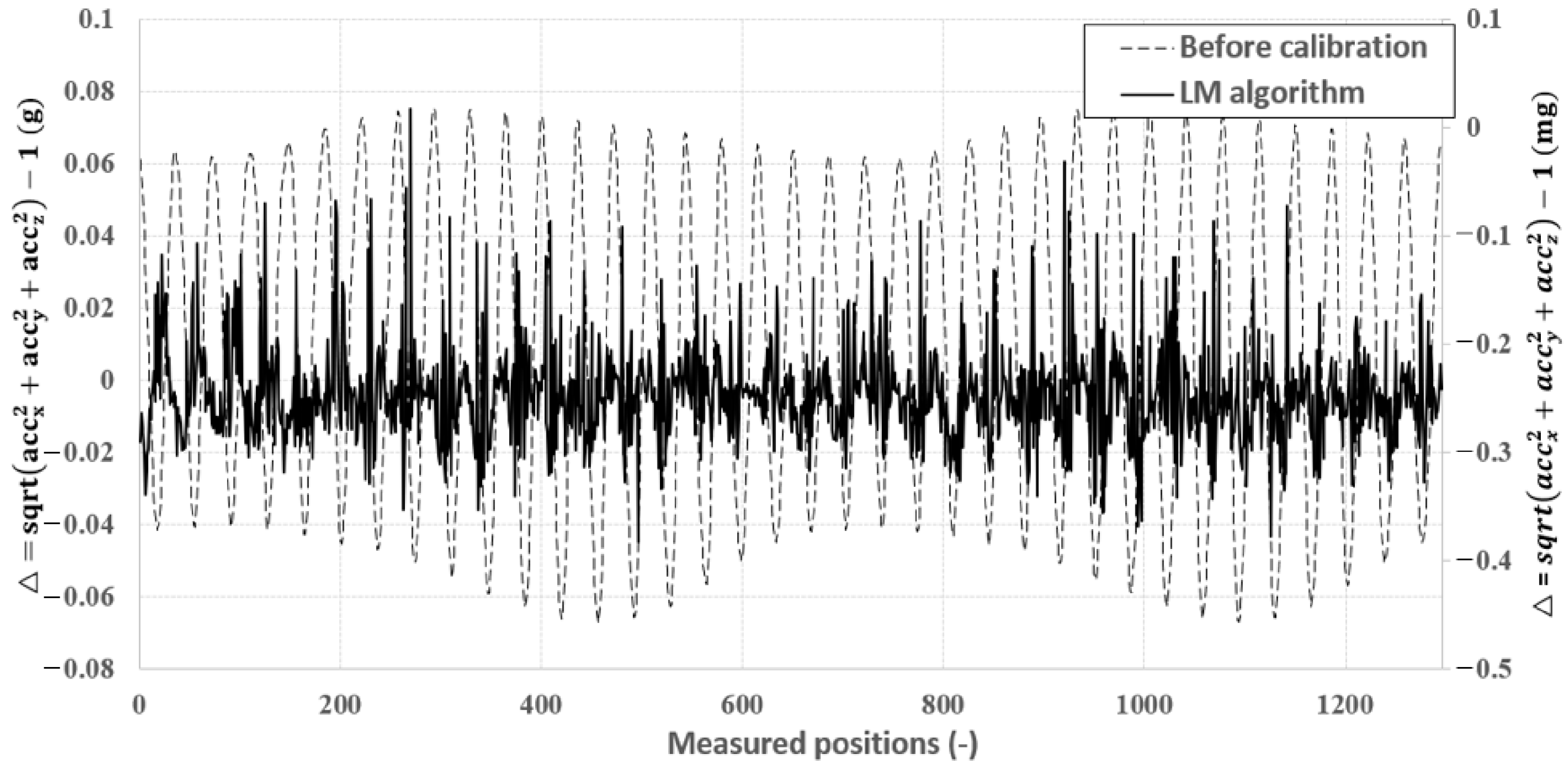
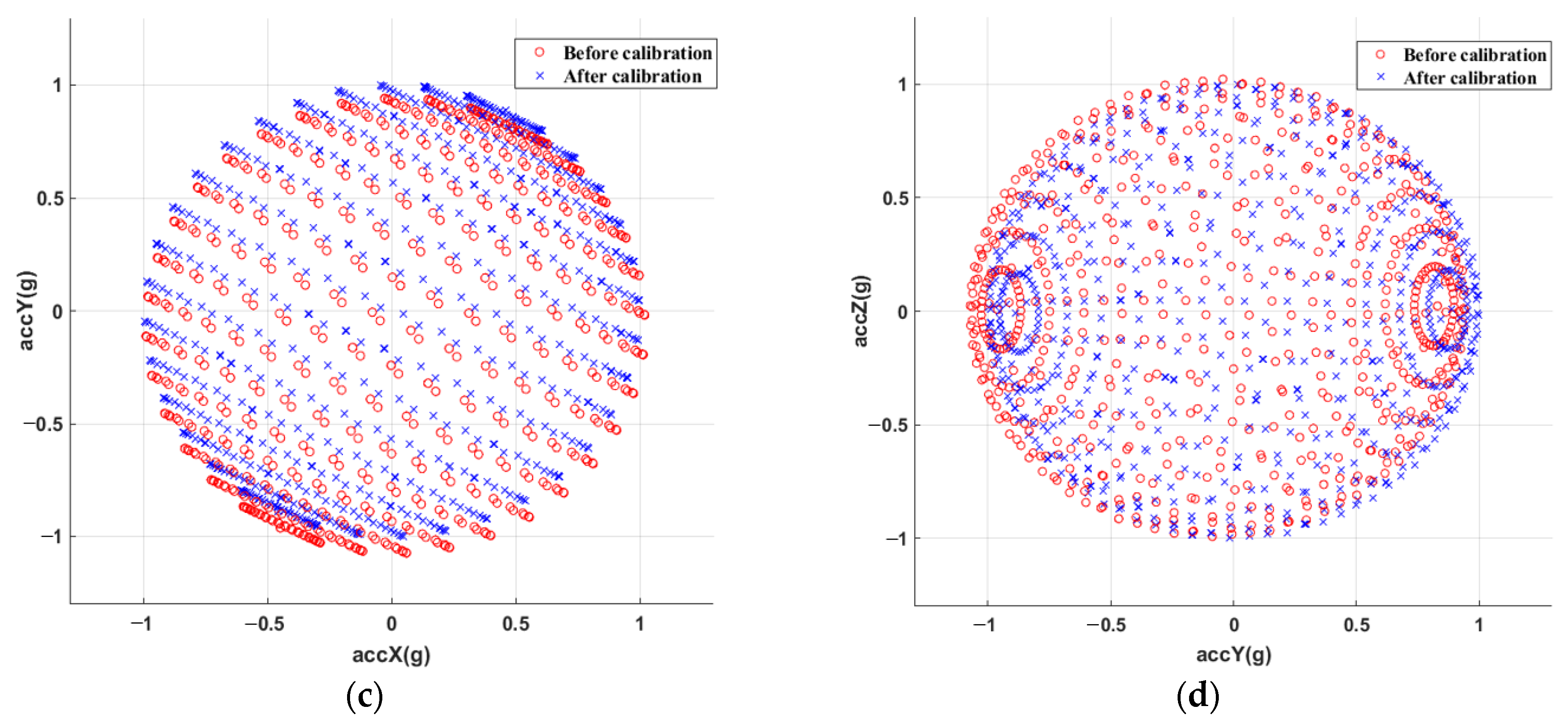
4.2. Sensor Frame Error Model Analyses
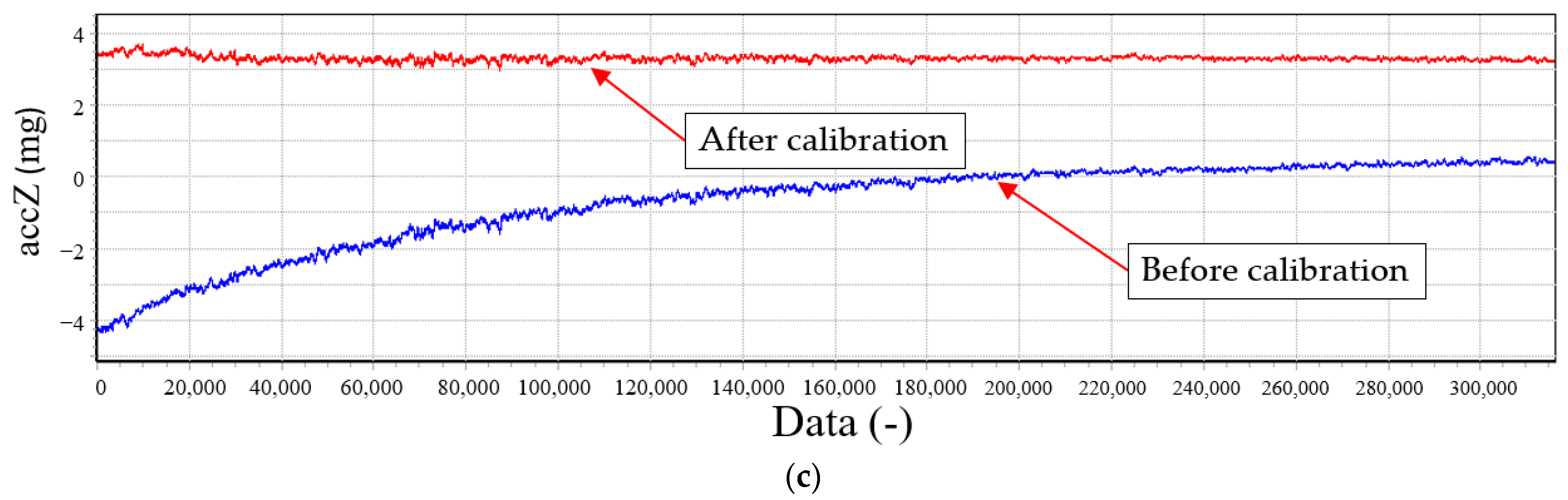
4.3. Temperature Compensation
5. Conclusions
Author Contributions
Funding
Institutional Review Board Statement
Informed Consent Statement
Data Availability Statement
Conflicts of Interest
References
- Liu, Q. Human motion state recognition based on MEMS sensors and Zigbee network. Comput. Commun. 2022, 181, 164–172. [Google Scholar] [CrossRef]
- Johnson, B.; Albrecht, C.; Braman, T.; Christ, K.; Duffy, P.; Endean, D.; Gnerlich, M.; Reinke, J. Development of a navigation-grade MEMS IMU. In Proceedings of the 2021 IEEE International Symposium on Inertial Sensors and Systems (INERTIAL), Virtual Format, 22–25 March 2021; IEEE: Piscataway, NJ, USA, 2021; pp. 1–4. [Google Scholar]
- Fontanarosa, D.; Francioso, L.; De Giorgi, M.G.; Vetrano, M.R. MEMS Vaporazing Liquid Microthruster: A Comprehensive Review. Appl. Sci. 2021, 11, 8954. [Google Scholar] [CrossRef]
- Gaber, K.; El_Mashade, M.B.; Aziz, G.A.A. Hardware-in-the-loop real-time validation of micro-satellite attitude control. Comput. Electr. Eng. 2020, 85, 106679. [Google Scholar] [CrossRef]
- Iasechko, M.; Shelukhin, O.; Maranov, A.; Lukianenko, S.; Basarab, O.; Hutchenko, O. Evaluation of the use of inertial navigation systems to improve the accuracy of object navigation. Int. J. Comput. Sci. Netw. Secur. 2021, 21, 71–75. [Google Scholar]
- Morales, J.J.; Khalife, J.; Abdallah, A.A.; Ardito, C.T.; Kassas, Z.M. Inertial navigation system aiding with Orbcomm LEO satellite Doppler measurements. In Proceedings of the 31st International Technical Meeting of the Satellite Division of The Institute of Navigation, Miami, FL, USA, 24–28 September 2018. [Google Scholar]
- Al-Masri WM, F.; Abdel-Hafez, M.F.; Jaradat, M.A. Inertial navigation system of pipeline inspection gauge. IEEE Trans-Actions Control Syst. Technol. 2018, 28, 609–616. [Google Scholar] [CrossRef]
- Zhu, M.; Pang, L.; Xiao, Z.; Shen, C.; Cao, H.; Shi, Y.; Liu, J. Temperature drift compensation for High-G MEMS accelerometer based on RBF NN im-proved method. Appl. Sci. 2019, 9, 695. [Google Scholar] [CrossRef]
- Wang, Y.; Zhang, J.; Yao, Z.; Lin, C.; Zhou, T.; Su, Y.; Zhao, J. A MEMS resonant accelerometer with high performance of temperature based on elec-trostatic spring softening and continuous ring-down technique. IEEE Sens. J. 2018, 18, 7023–7031. [Google Scholar] [CrossRef]
- He, J.; Zhou, W.; Yu, H.; He, X.; Peng, P. Structural designing of a MEMS capacitive accelerometer for low temperature coefficient and high linearity. Sensors 2018, 18, 643. [Google Scholar] [CrossRef]
- Wang, X.; Xu, W.; Lee, Y.K. An ambient temperature compensated microthermal convective accelerometer with high sen-sitivity stability. In Proceedings of the 2019 20th International Conference on Solid-State Sensors, Actuators and Microsystems & Eu-rosensors XXXIII (TRANSDUCERS & EUROSENSORS XXXIII), Berlin, Germany, 23–27 June 2019; IEEE: Piscataway, NJ, USA, 2019; pp. 1827–1830. [Google Scholar]
- Wang, S.; Zhu, W.; Shen, Y.; Ren, J.; Gu, H.; Wei, X. Temperature compensation for MEMS resonant accelerometer based on genetic algorithm optimized backpropagation neural network. Sens. Actuators A Phys. 2020, 316, 112393. [Google Scholar] [CrossRef]
- Cui, S.; Cui, L.; Du, Y.; Chai, S.; Zhang, B. Calibration of MEMS accelerometer using kaiser filter and the ellipsoid fitting method. In Proceedings of the 2018 37th Chinese Control Conference (CCC), Wuhan, China, 25–27 July 2018; IEEE: Piscataway, NJ, USA, 2018. [Google Scholar]
- Xu, T.; Xu, X.; Xu, D.; Zhao, H. A novel calibration method using six positions for MEMS triaxial accelerometer. IEEE Trans. Instrum. Meas. 2021, 70, 1002211. [Google Scholar] [CrossRef]
- Chao, C.; Zhao, J.; Zhu, J.; Bessaad, N. Minimum settings calibration method for low-cost triaxial IMU and magnetometer. Meas. Sci. Technol. 2021, 33, 025103. [Google Scholar] [CrossRef]
- Zhu, J.; Wang, W.; Huang, S.; Ding, W. An improved calibration technique for mems accelerometer-based inclinometers. Sensors 2020, 20, 452. [Google Scholar] [CrossRef]
- Ngoh, K.J.H.; Gouwanda, D.; Gopalai, A.A.; Chong, Y.Z. Estimation of vertical ground reaction force during running using neural network model and uniaxial accelerometer. J. Biomech. 2018, 76, 269–273. [Google Scholar] [CrossRef]
- Khankalantary, S.; Ranjbaran, S.; Ebadollahi, S. Simplification of calibration of low-cost MEMS accelerometer and its tem-perature compensation without accurate laboratory equipment. Meas. Sci. Technol. 2021, 32, 045102. [Google Scholar] [CrossRef]
- Tkalich, V.L.; Labkovskaia, R.I.; Pirozhnikova, O.I.; Kalinkina, M.E.; Kozlov, A.S. Analysis of errors in micromechanical devices. In Proceedings of the 2018 XIV In-ternational Scientific-Technical Conference on Actual Problems of Electronics Instrument Engineering (APEIE), Novosibirsk, Russia, 2–6 October 2018; IEEE: Piscataway, NJ, USA, 2018. [Google Scholar]
- Zhao, H.; Wang, Y.; Liu, R.; Lin, F.; Gao, F.; Qiu, S.; Wang, Z. Calibration of Smartphone’s Integrated Magnetic and Inertial Measurement Units. In Proceedings of the 2021 33rd Chinese Control and Decision Conference (CCDC), Kunming, China, 22–24 May 2021; IEEE: Piscataway, NJ, USA, 2021. [Google Scholar]
- Chang, H.T.; Chang, J.Y. Iterative robust ellipsoid fitting based on Mestimator with geometry radius constraint. IEEE Sens. J. 2022, 23, 1397–1407. [Google Scholar]
- Ibrahim, A.; Eltawil, A.; Na, Y.; El-Tawil, S. Accuracy limits of embedded smart device accelerometer sensors. IEEE Trans. Instrum. Meas. 2020, 69, 5488–5496. [Google Scholar] [CrossRef]
- Shen, Q.; Yang, D.; Zhou, J.; Wu, Y.; Zhang, Y.; Yuan, W. A Measurement-Data-Driven Control Approach towards Variance Reduction of Microm-achined Resonant Accelerometer under Multi Unknown Disturbances. Micromachines 2019, 10, 294. [Google Scholar] [CrossRef]
- Hoang, M.L.; Pietrosanto, A. A new technique on vibration optimization of industrial inclinometer for MEMS accelerometer without sensor fusion. IEEE Access 2021, 9, 20295–20304. [Google Scholar] [CrossRef]
- Niu, X.; Li, Y.; Zhang, H.; Wang, Q.; Ban, Y. Fast thermal calibration of low-grade inertial sensors and inertial measurement units. Sensors 2013, 13, 12192–12217. [Google Scholar] [CrossRef]
- Ru, X.; Gu, N.; Shang, H.; Zhang, H. MEMS inertial sensor calibration technology: Current status and future trends. Micromachines 2022, 13, 879. [Google Scholar] [CrossRef]
- Song, Z.; Cao, Z.; Li, Z.; Wang, J.; Liu, Y. Inertial motion tracking on mobile and wearable devices: Recent advancements and challenges. Tsinghua Sci. Technol. 2021, 26, 692–705. [Google Scholar] [CrossRef]
- Xu, D.; Yang, Z.; Zhao, H.; Zhou, X. A temperature compensation method for MEMS accelerometer based on LM_BP neural network. In Proceedings of the 2016 IEEE Sensors, Catania, Italy, 20–22 April 2016. [Google Scholar]
- Kose, T.; Azgin, K.; Akin, T. Temperature compensation of a capacitive MEMS accelerometer by using a MEMS oscilla-tor. In Proceedings of the 2016 IEEE International Symposium on Inertial Sensors and Systems, Laguna Beach, CA, USA, 22 February 2016. [Google Scholar]
- Guo, X.; Yang, W.; Zheng, T.; Sun, J.; Xiong, X.; Wang, Z.; Zou, X. Input-Output-Improved Reservoir Computing Based on Duffing Resonator Processing Dynamic Temperature Compensation for MEMS Resonant Accelerometer. Micromachines 2023, 14, 161. [Google Scholar] [CrossRef] [PubMed]
- Ruzza, G.; Guerriero, L.; Revellino, P.; Guadagno, F.M. Thermal compensation of low-cost MEMS accelerometers for tilt measurements. Sensors 2018, 18, 2536. [Google Scholar] [CrossRef] [PubMed]
- Lee, H.J.; Park, D.J. Analysis of Thermal Characteristics of MEMS Sensors for Measuring the Rolling Period of Maritime Autonomous Surface Ships. J. Mar. Sci. Eng. 2022, 10, 859. [Google Scholar] [CrossRef]
- Gheorghe, M.V. Advanced calibration method for 3-axis MEMS accelerometers. In Proceedings of the 2016 International Semiconductor Conference (CAS), Sinaia, Romania, 10–12 October 2016; IEEE: Piscataway, NJ, USA, 2016. [Google Scholar]
- Araghi, G.; Landry, R.J. Temperature compensation model of MEMS inertial sensors based on neural network. In Proceedings of the 2018 IEEE/ION Position, Location and Navigation Symposium (PLANS), Monterey, CA, USA, 23–26 April 2018; pp. 301–309. [Google Scholar]
- Xu, L.; Wang, S.; Jiang, Z.; Wei, X. Programmable synchronization enhanced MEMS resonant accelerometer. Microsyst. Nanoeng. 2020, 6, 1–10. [Google Scholar] [CrossRef] [PubMed]
- Jalal, A.; Quaid, M.A.K.; Tahir, S.B.U.D.; Kim, K. A study of accelerometer and gyroscope measurements in physical life-log activities detection systems. Sensors 2020, 20, 6670. [Google Scholar] [CrossRef] [PubMed]
- Migueles, J.H.; Rowlands, A.V.; Huber, F.; Sabia, S.; van Hees, V.T. GGIR: A research community–driven open source R package for generating physical activity and sleep outcomes from multi-day raw accelerometer data. J. Meas. Phys. Behav. 2019, 2, 188–196. [Google Scholar] [CrossRef]
- John, D.; Tang, Q.; Albinali, F.; Intille, S. An open-source monitor-independent movement summary for accelerometer data processing. J. Meas. Phys. Behav. 2019, 2, 268–281. [Google Scholar] [CrossRef]
- Ren, S.Q.; Liu, Q.B.; Zeng, M.; Wang, C.H. Calibration method of accelerometer’s high-order error model coefficients on precision centrifuge. IEEE Trans. Instrum. Meas. 2019, 69, 2277–2286. [Google Scholar] [CrossRef]
- Li, Y.; Georgy, J.; Niu, X.; Li, Q.; El-Sheimy, N. Autonomous calibration of MEMS gyros in consumer portable devices. IEEE Sens. J. 2015, 15, 4062–4072. [Google Scholar] [CrossRef]
- Ranjbaran, S.; Ebadollahi, S. Fast and precise solving of non-linear optimisation problem for field calibration of triaxial accelerometer. Electron. Lett. 2018, 54, 148–150. [Google Scholar] [CrossRef]
- Wu, H.; Pei, X.; Li, J.; Gao, H.; Bai, Y. An improved magnetometer calibration and compensation method based on Levenberg–Marquardt algorithm for multi-rotor unmanned aerial vehicle. Meas. Control 2020, 53, 276–286. [Google Scholar] [CrossRef]
- Cuadrado, J.; Michaud, F.; Lugrís, U.; Pérez Soto, M. Using accelerometer data to tune the parameters of an extended kalman filter for optical motion capture: Preliminary application to gait analysis. Sensors 2021, 21, 427. [Google Scholar] [CrossRef] [PubMed]
- Sarkka, O.; Nieminen, T.; Suuriniemi, S.; Kettunen, L. A multi-position calibration method for consumer-grade accelerometers, gyroscopes, and magnetometers to field conditions. IEEE Sens. J. 2017, 17, 3470–3481. [Google Scholar] [CrossRef]
- Zhang, P.; Li, Y.; Zhuang, Y.; Kuang, J.; Niu, X.; Chen, R. Multi-level information fusion with motion constraints: Key to achieve high-precision gait analysis using low-cost inertial sensors. Inf. Fusion 2023, 89, 603–618. [Google Scholar] [CrossRef]
- Yang, J.; Wu, W.; Wu, Y.; Lian, J. Thermal calibration for the accelerometer triad based on the sequential multiposition observation. IEEE Trans. Instrum. Meas. 2012, 62, 467–482. [Google Scholar] [CrossRef]
- Alfian, R.I.; Ma’arif, A.; Sunardi, S. Noise reduction in the accelerometer and gyroscope sensor with the Kalman filter al-gorithm. J. Robot. Control 2021, 2, 180–189. [Google Scholar]
- Wang, Y.; Li, Z.; Li, X. External disturbances rejection for vector field sensors in attitude and heading reference systems. Micromachines 2020, 11, 803. [Google Scholar] [CrossRef]
- Shandhi, M.M.H.; Semiz, B.; Hersek, S.; Goller, N.; Ayazi, F.; Inan, O.T. Performance analysis of gyroscope and accelerometer sensors for seismocar-diography-based wearable pre-ejection period estimation. IEEE J. Biomed. Health Inform. 2019, 23, 2365–2374. [Google Scholar] [CrossRef]
- Han, Z.; Hong, L.; Meng, J.; Li, Y.; Gao, Q. Temperature drift modeling and compensation of capacitive accelerometer based on AGA-BP neural network. Measurement 2020, 164, 108019. [Google Scholar] [CrossRef]
- Xu, T.; Xu, X.; Xu, D.; Zou, Z.; Zhao, H. Low-Cost and Efficient Thermal Calibration Scheme for MEMS Triaxial Accelerometer. IEEE Trans. Instrum. Meas. 2021, 70, 1–9. [Google Scholar] [CrossRef]


| No. | X Axis Position | Y Axis Position | Z Axis Position |
|---|---|---|---|
| 1 | Px1 ≈ horizontal | Py1 ≈ vertical | Pz1 ≈ horizontal |
| 2 | Px1 + 45° | Py1 + 45° | Pz1 |
| 3 | Px1 + 90° | Py1 + 90° | Pz1 |
| 4 | Px1 + 135° | Py1 + 135° | Pz1 |
| 5 | Px1 + 180° | Py1 + 180° | Pz1 |
| 6 | Px1 + 225° | Py1 + 225° | Pz1 |
| 7 | Px1 + 270° | Py1 + 270° | Pz1 |
| 8 | Px1 + 315° | Py1 + 315° | Pz1 |
| 9 | Px2 ≈ horizontal | Py2 ≈ horizontal | Pz2 ≈ vertical |
| 10 | Px2 + 45° | Py2 | Pz2 + 45° |
| 11 | Px2 + 90° | Py2 | Pz2 + 90° |
| 12 | Px2 + 135° | Py2 | Pz2 + 135° |
| 13 | Px2 + 180° | Py2 | Pz2 + 180° |
| 14 | Px2 + 225° | Py2 | Pz2 + 225° |
| 15 | Px2 + 270° | Py2 | Pz2 + 270° |
| 16 | Px2 + 315° | Py2 | Pz2 + 315° |
| 17 | Px3 ≈ horizontal | Py3 ≈ horizontal | Pz3 ≈ vertical |
| 18 | Px3 | Py3 + 45° | Pz3 + 45° |
| 19 | Px3 | Py3 + 90° | Pz3 + 90° |
| 20 | Px3 | Py3 + 135° | Pz3 + 135° |
| 21 | Px3 | Py3 + 180° | Pz3 + 180° |
| 22 | Px3 | Py3 + 225° | Pz3 + 225° |
| 23 | Px3 | Py3 + 270° | Pz3 + 270° |
| 24 | Px3 | Py3 + 315° | Pz3 + 315° |
| Specification | Value |
|---|---|
| Interface | Digital |
| Noise-Density (μg/) | 25 |
| 0 g Offset (mg) | ±25 |
| Range (g) | ±2/±4/±8 |
| ADC | 20-bit |
| Output Data Rate (Hz) | 0~4000 Hz |
| Turntable | |
|---|---|
| Principal axis rotation range | Continuous infinite |
| Tilting axis angular position accuracy | ±3″ |
| Principal axis angular position accuracy | ±3″ |
| Non-orthogonalities between axes | ±5″ |
| Tilting axis rotation range | ±90° |
| Thermal Chamber | |
| Temperature range | −55~+100 °C |
| Temperature change rate | ±0.1~±5 °C/min linear |
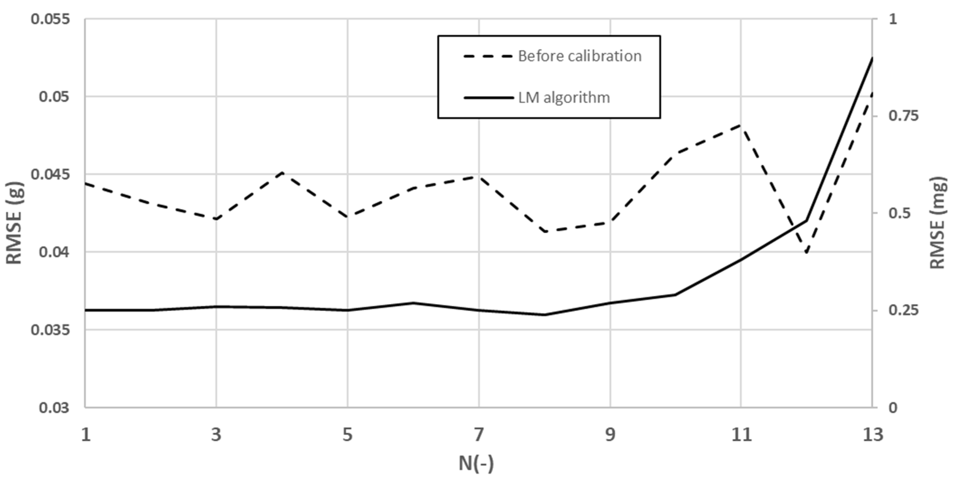
| N | NoP | N | NoP | N | NoP |
|---|---|---|---|---|---|
| 1 | 1296 | 6 | 64 | 11 | 18 |
| 2 | 648 | 7 | 48 | 12 | 16 |
| 3 | 324 | 8 | 36 | 13 | 12 |
| 4 | 162 | 9 | 24 | ||
| 5 | 81 | 10 | 21 |
| Reference Angle | Without Calibration | After Calibration | SEOQ |
|---|---|---|---|
| 0; 0 | −0.77; 0.59 | −0.70; −0.30 | 0.2; 3.0 |
| 15; 0 | 14.18; −0.62 | 14.61; −0.15 | 1.4; 1.6 |
| 30; 0 | 29.18; −0.63 | 30.13; 0.01 | 3.2; 2.1 |
| 0; −15 | −0.96; −15.83 | −0.91; −15.72 | 0.2; 0.4 |
| 0; −30 | −0.82; −31.10 | −0.76; −31.00 | 0.2; 0.3 |
| 15; −15 | 14.31; −15.98 | 14.76; −15.82 | 1.5; 0.5 |
| 30; −30 | 29.00; −29.62 | 29.98; −29.76 | 3.3; 0.5 |
| Temperature (°C) | Before Calibration RMSE (mg) | Polynomial RMSE (mg) | Measurement RMSE (mg) |
|---|---|---|---|
| −35 | 45.1 | 0.19 | 0.17 |
| −25 | 46.8 | 0.24 | 0.21 |
| −15 | 47.2 | 0.22 | 0.19 |
| −5 | 45.9 | 0.24 | 0.21 |
| 5 | 44.3 | 0.18 | 0.17 |
| 15 | 46.3 | 0.19 | 0.21 |
| 25 | 48.6 | 0.25 | 0.25 |
| 35 | 47.2 | 0.26 | 0.29 |
| 45 | 45.3 | 0.29 | 0.24 |
| 55 | 48.1 | 0.31 | 0.29 |
Disclaimer/Publisher’s Note: The statements, opinions and data contained in all publications are solely those of the individual author(s) and contributor(s) and not of MDPI and/or the editor(s). MDPI and/or the editor(s) disclaim responsibility for any injury to people or property resulting from any ideas, methods, instructions or products referred to in the content. |
© 2023 by the authors. Licensee MDPI, Basel, Switzerland. This article is an open access article distributed under the terms and conditions of the Creative Commons Attribution (CC BY) license (https://creativecommons.org/licenses/by/4.0/).
Share and Cite
Yuan, B.; Tang, Z.; Zhang, P.; Lv, F. Thermal Calibration of Triaxial Accelerometer for Tilt Measurement. Sensors 2023, 23, 2105. https://doi.org/10.3390/s23042105
Yuan B, Tang Z, Zhang P, Lv F. Thermal Calibration of Triaxial Accelerometer for Tilt Measurement. Sensors. 2023; 23(4):2105. https://doi.org/10.3390/s23042105
Chicago/Turabian StyleYuan, Bo, Zhifeng Tang, Pengfei Zhang, and Fuzai Lv. 2023. "Thermal Calibration of Triaxial Accelerometer for Tilt Measurement" Sensors 23, no. 4: 2105. https://doi.org/10.3390/s23042105
APA StyleYuan, B., Tang, Z., Zhang, P., & Lv, F. (2023). Thermal Calibration of Triaxial Accelerometer for Tilt Measurement. Sensors, 23(4), 2105. https://doi.org/10.3390/s23042105