
The Effect of Soil-Structure Interaction on the Seismic Response of Structures Using Machine Learning, Finite Element Modeling and ASCE 7-16 Methods


Abstract
:1. Introduction
2. Methodology
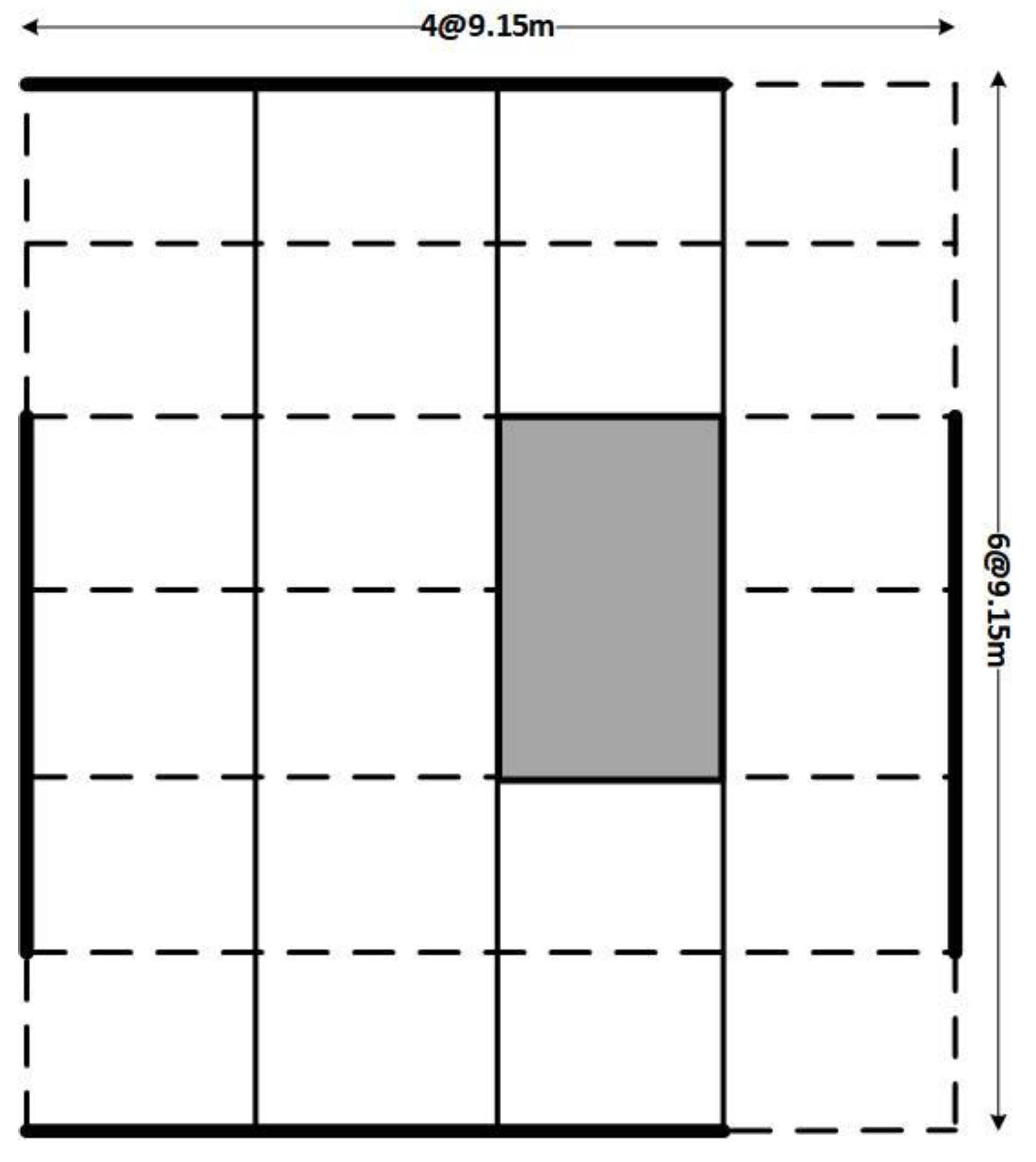
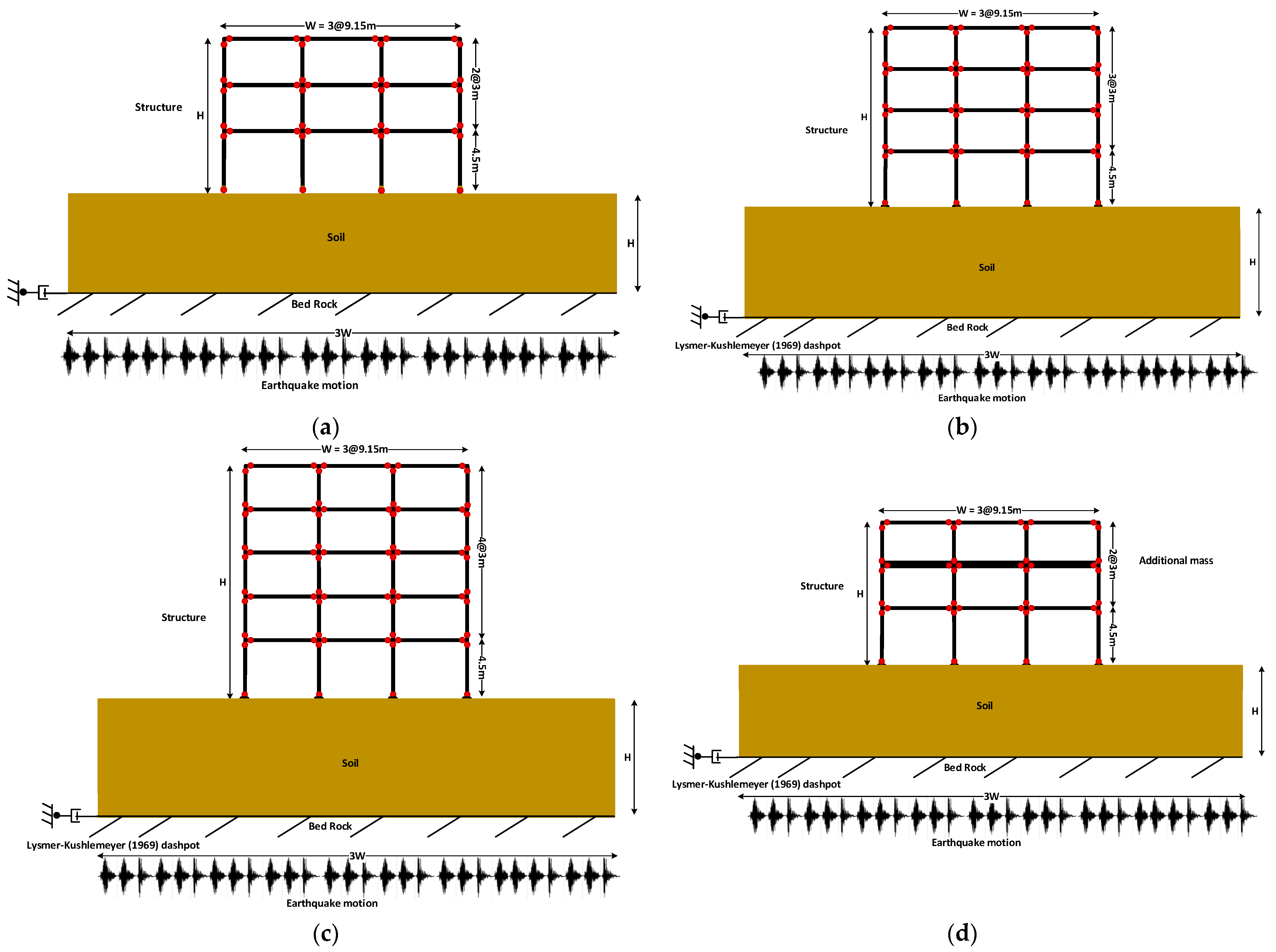
2.1. Modeling the Superstructure (Building)
2.2. Modeling the Substructure (Soil)
2.3. Modeling of the Earthquakes
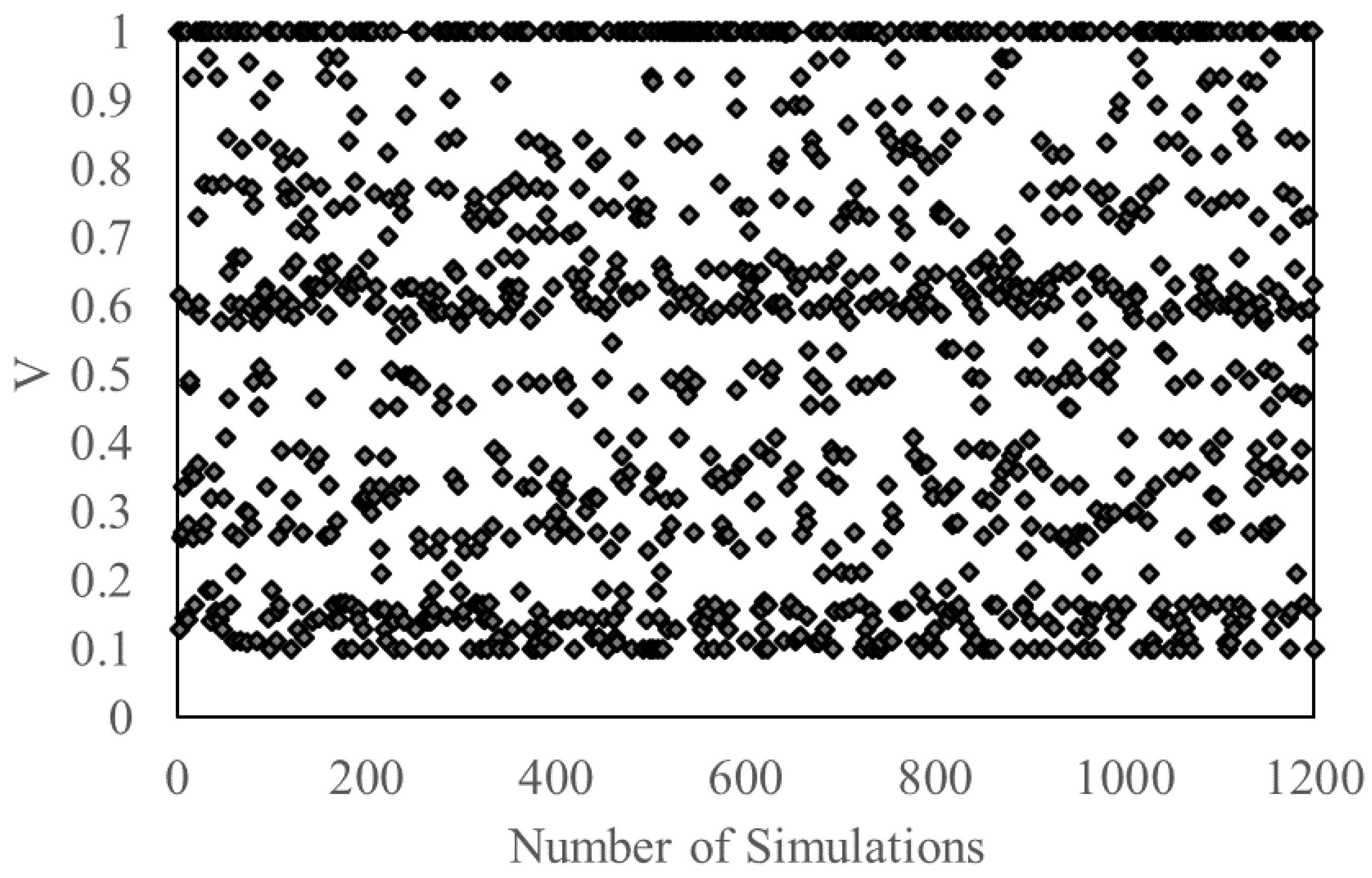
2.4. Database for Machine Learning Methods
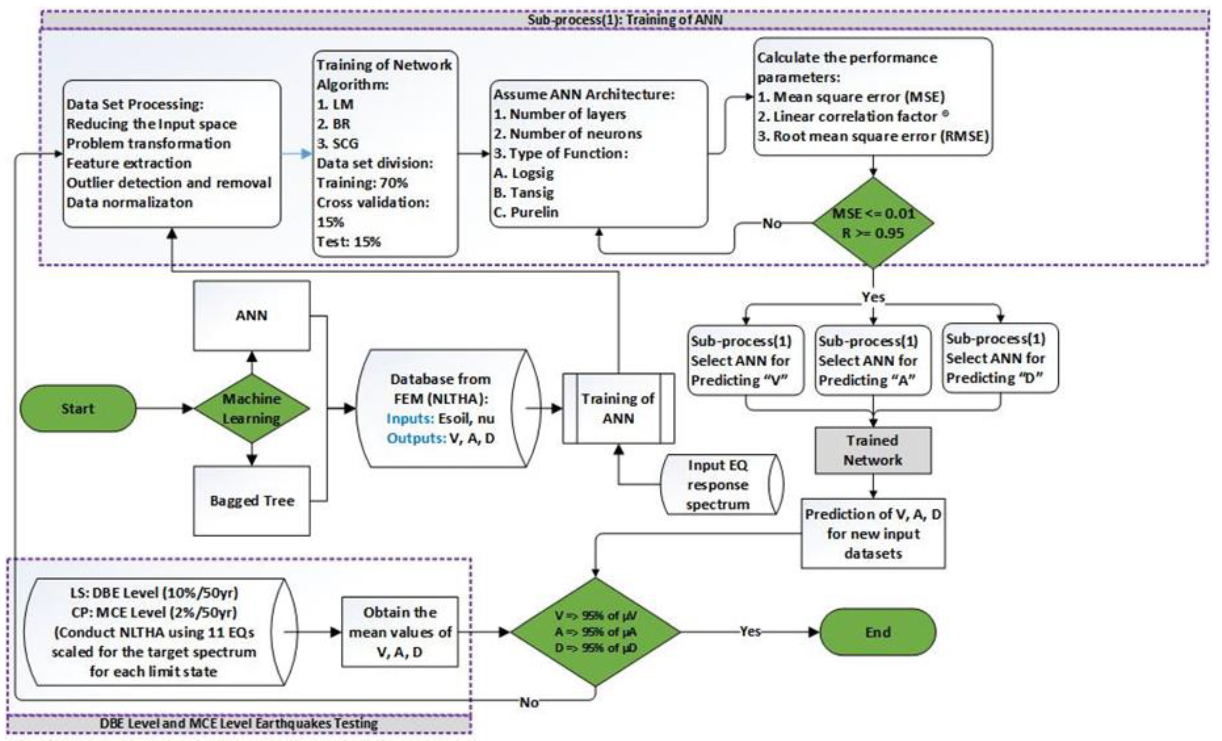
2.5. Implementing the Machine Learning Techniques
3. Application of the Machine Learning techniques
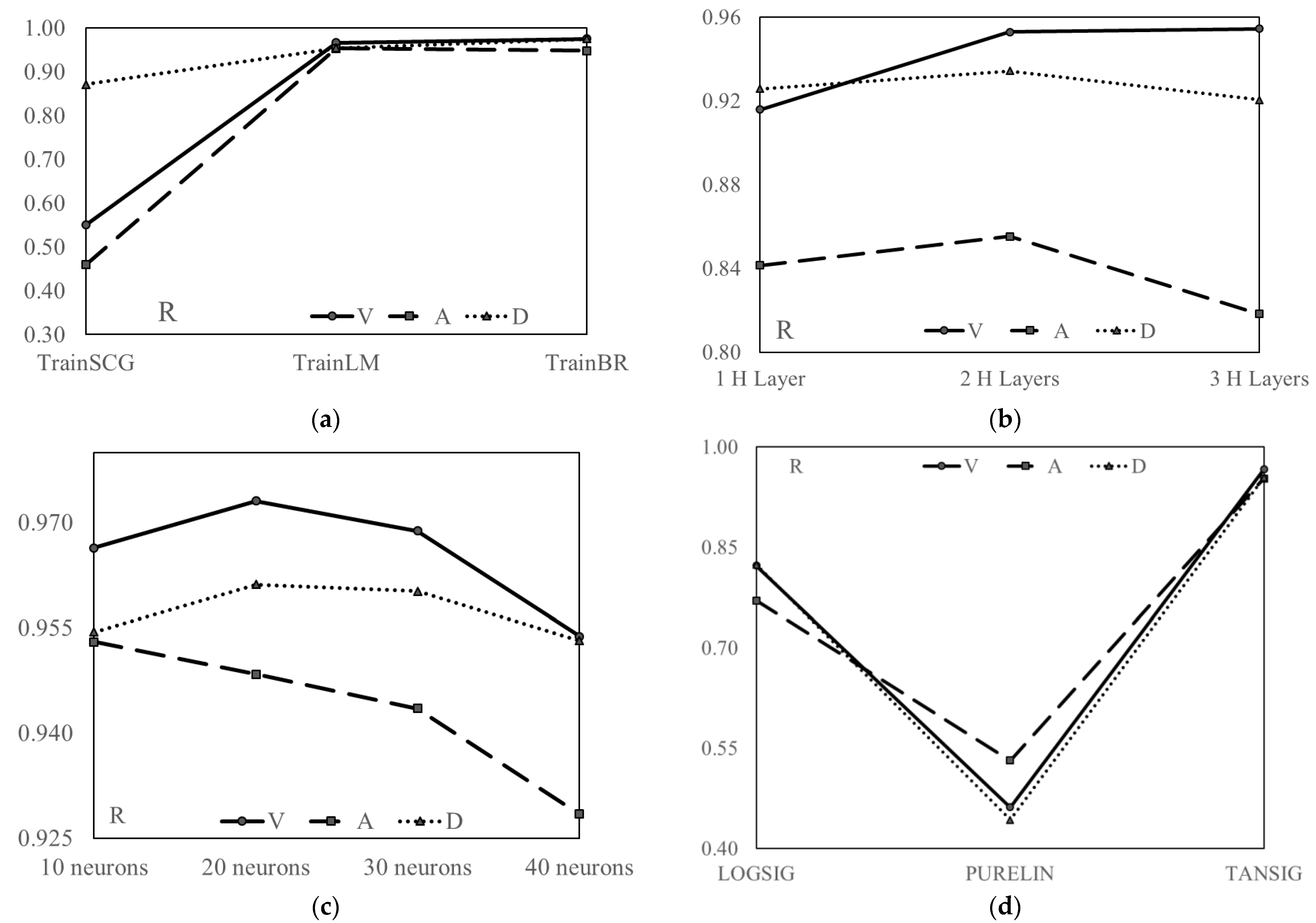
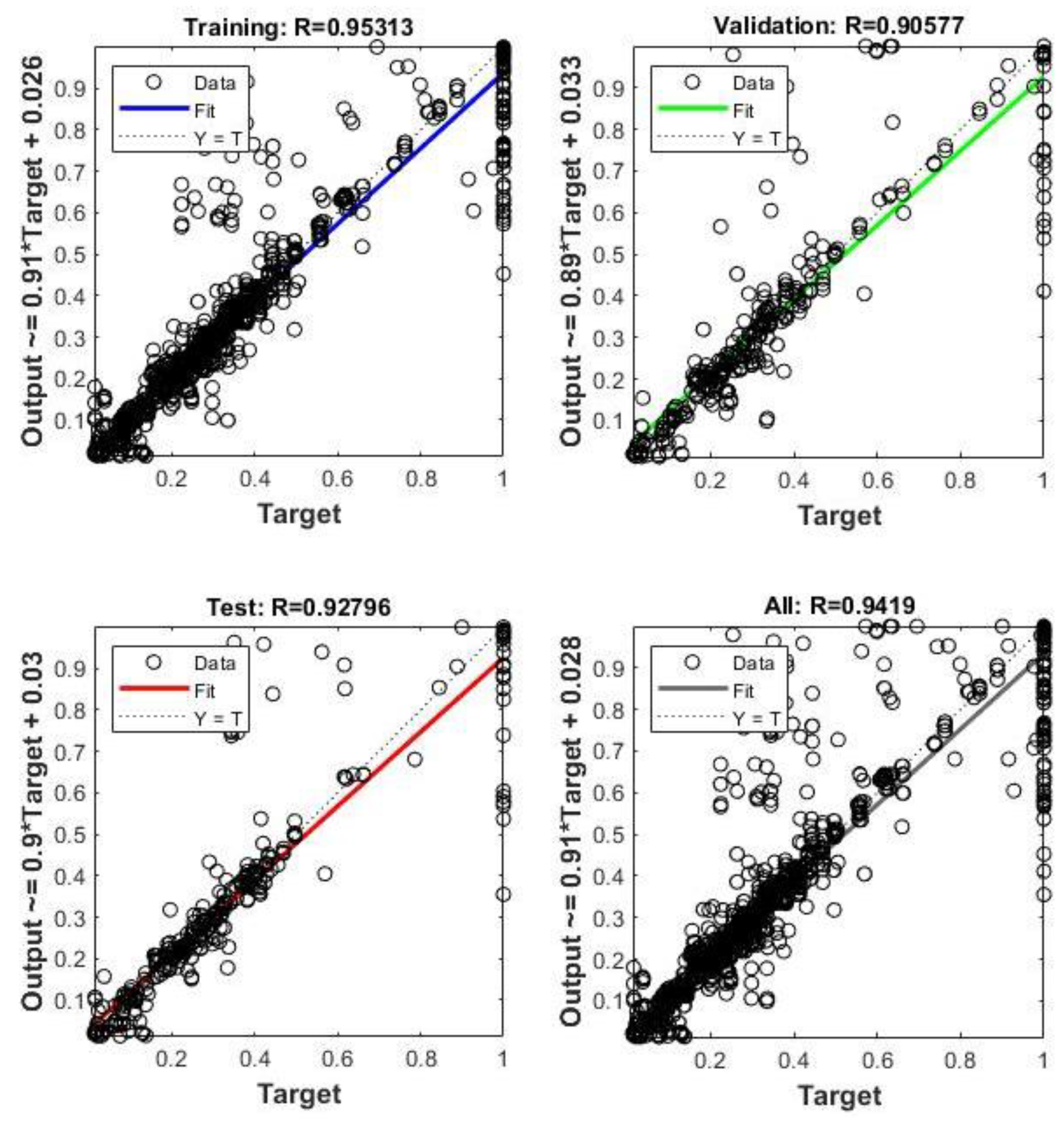
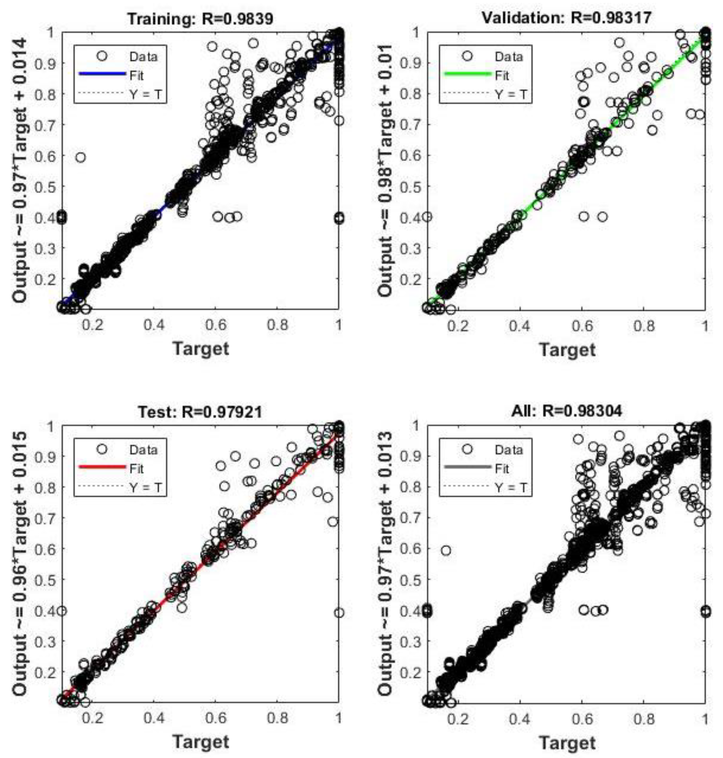
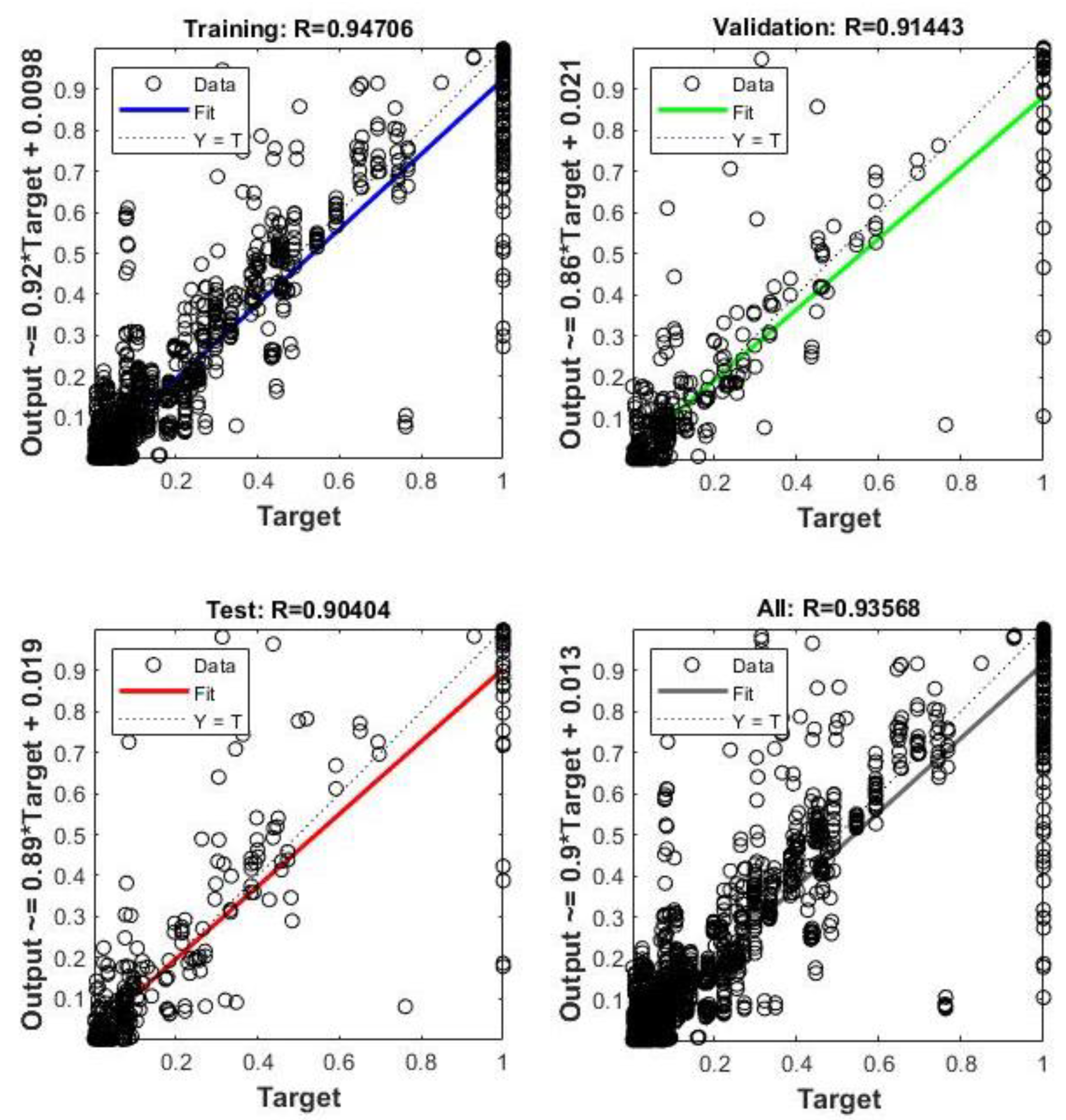
3.1. Training and Test of the ANNs
3.2. Training and Test of the Support Vector Machines (SVMs)
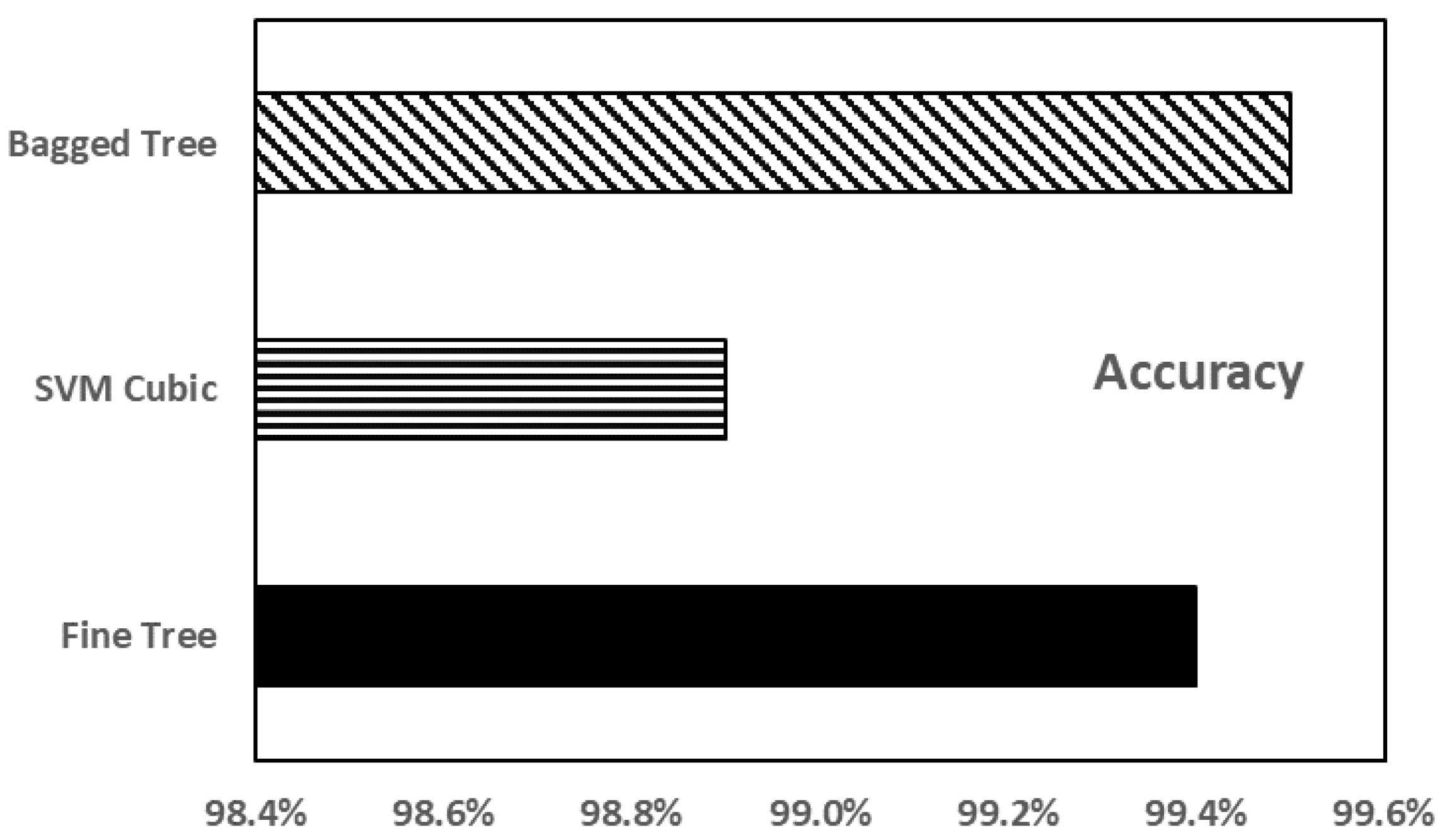
3.3. Comparison of the Performance of the ML Techniques
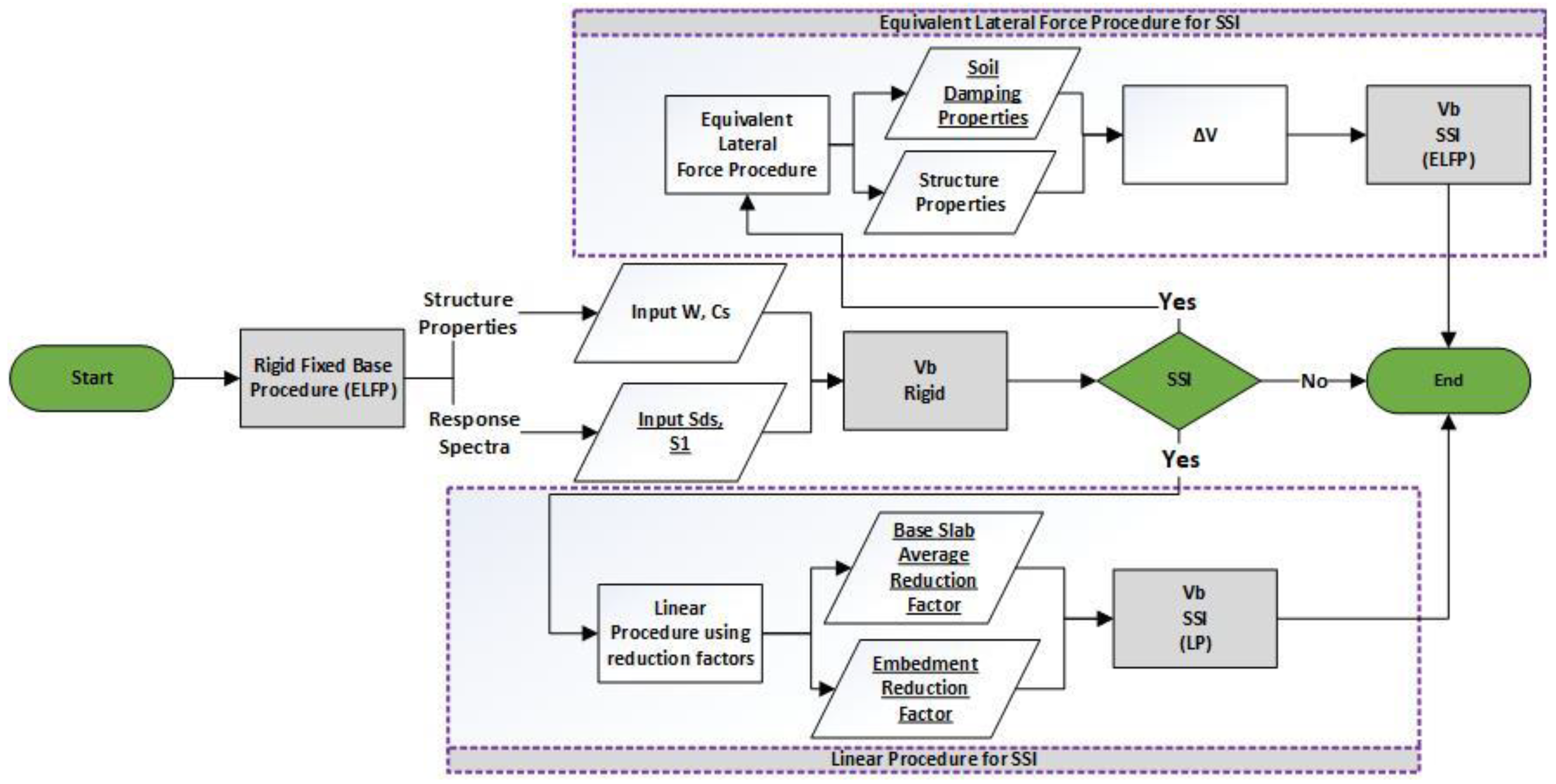
4. ASCE 7-16 Methodology
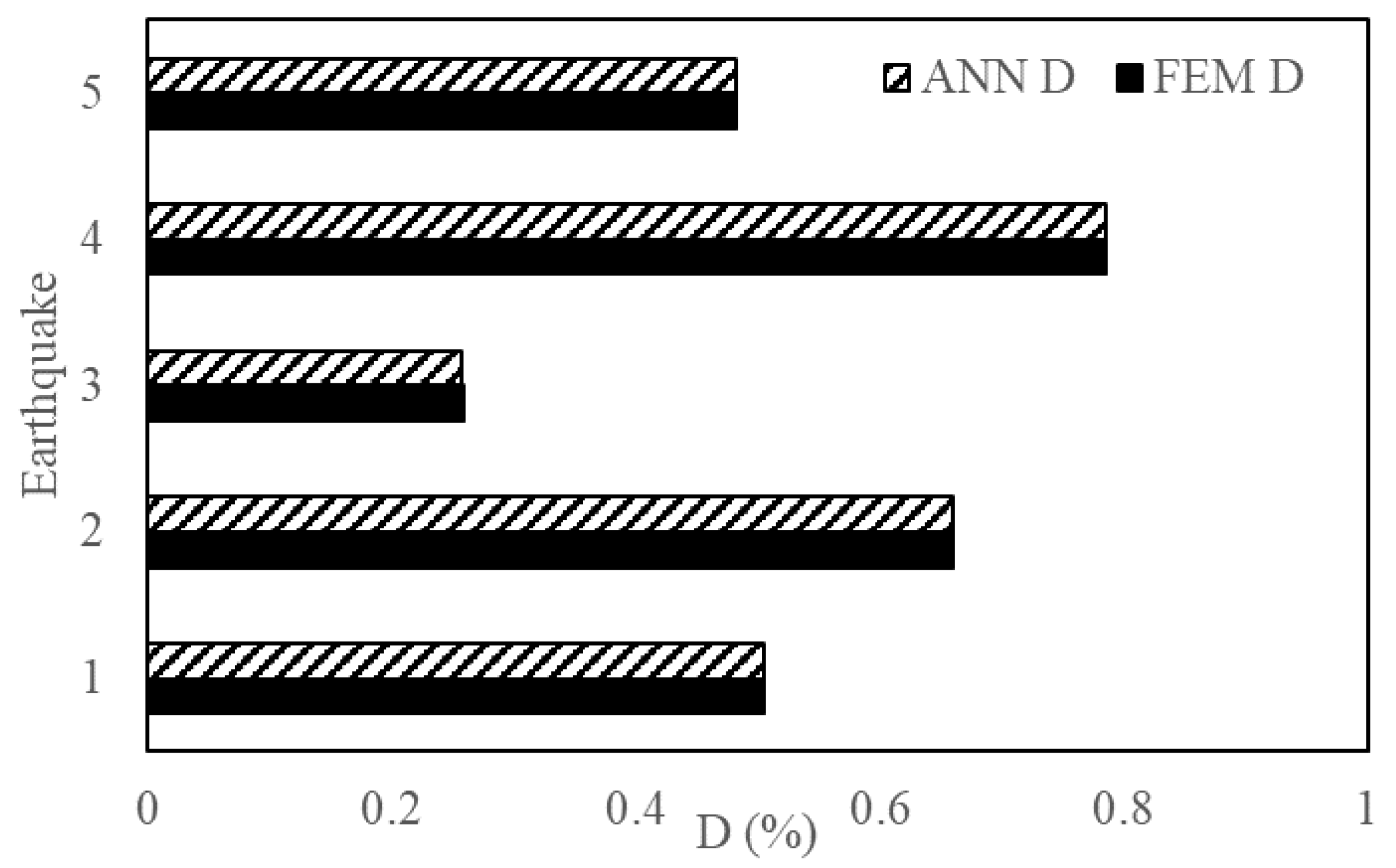
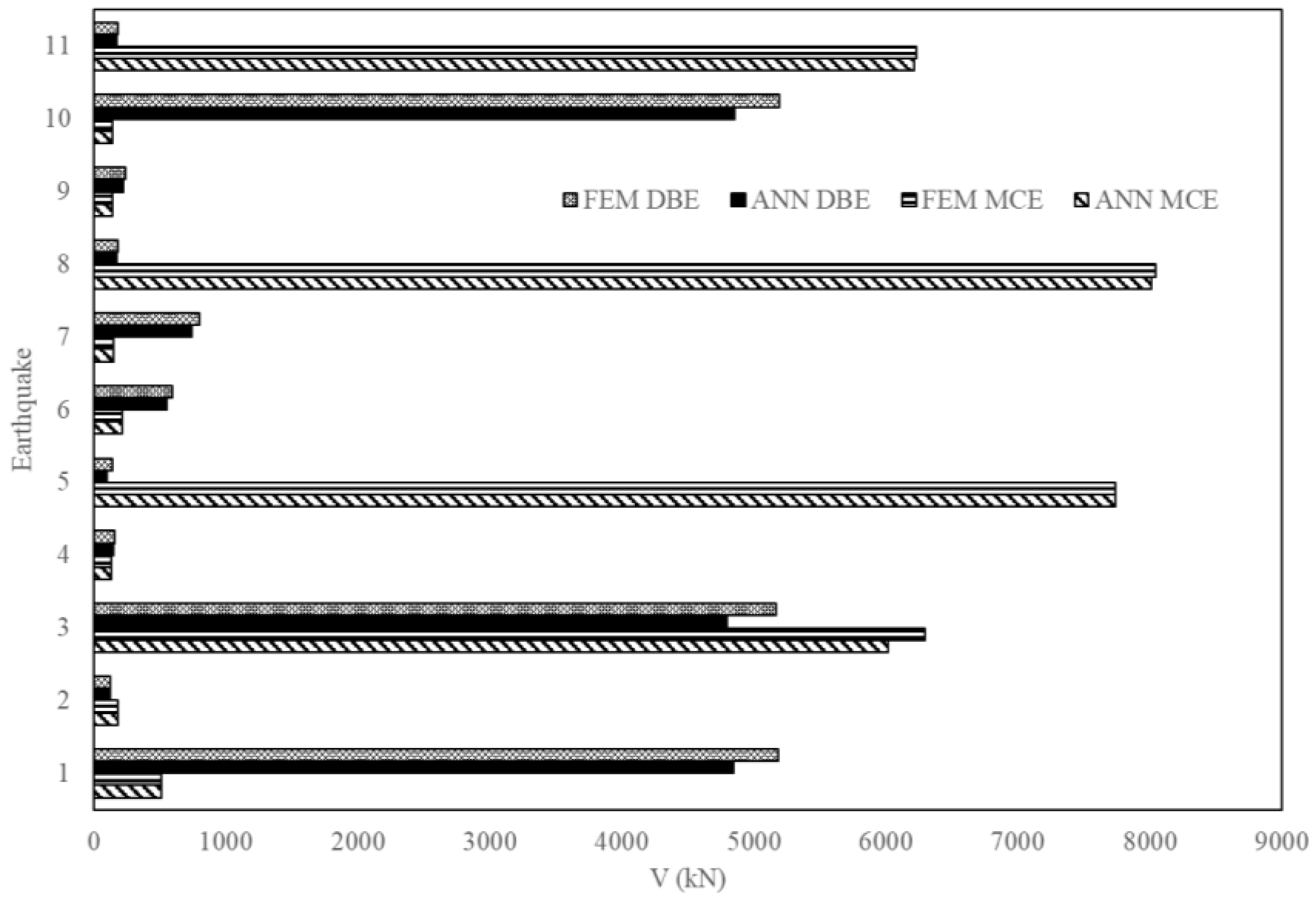
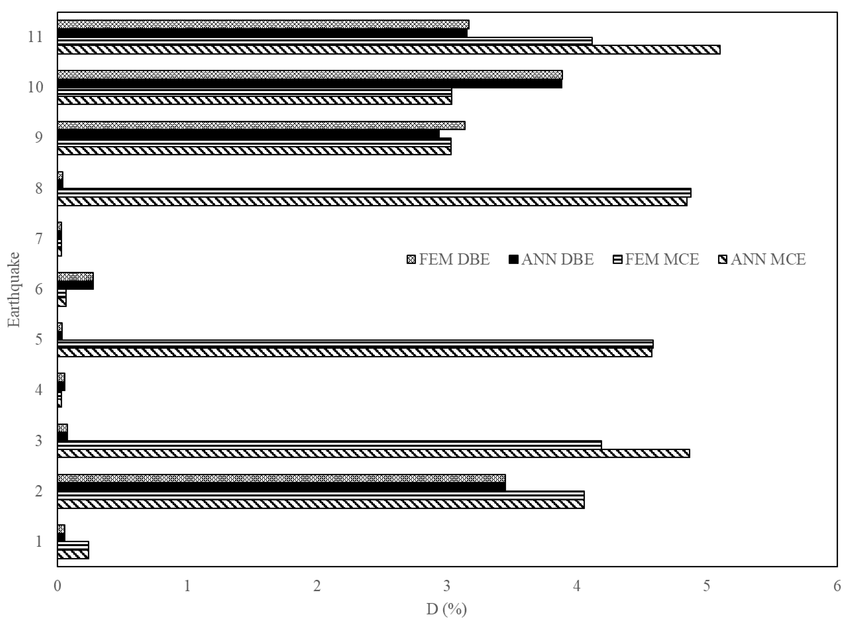
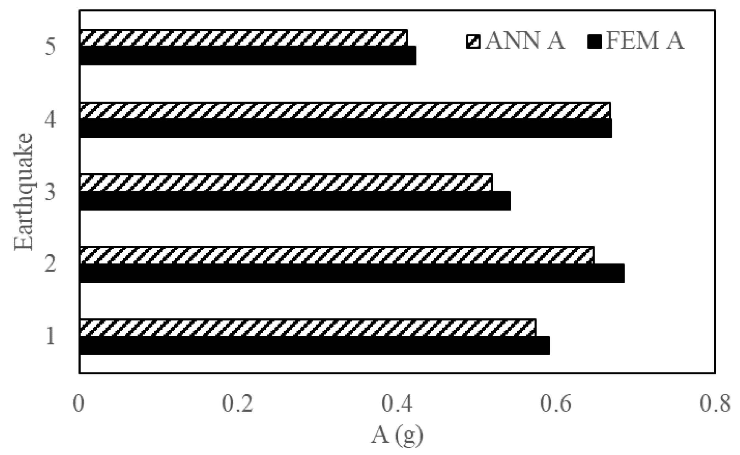
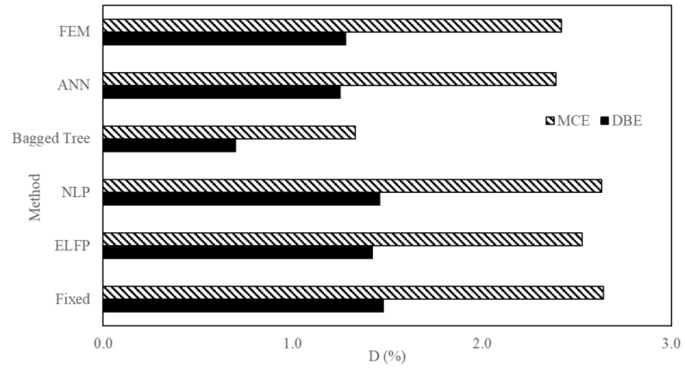
5. Results and Discussion
6. Conclusions
- The machine learning framework achieved more than 95% accuracy with two layers having ten neurons each, TANSIG function and TrainLM algorithm.
- The soil-structure-interaction-based artificial neural network model results were in good agreement with those of the nonlinear time history analysis compared with fixed-base, support vector machine and ASCE 7-16 linear soil-structure interaction methods.
- The errors in artificial neural network predictions were less than 2% for the maximum considered earthquake and below 8% for the design-based earthquake with nonlinear time history analysis as a reference.
- One of the interesting finding is that the artificial neural network framework provided higher accuracy in predicting base shear and drift compared with conventional ASCE methods.
- The proposed framework showed high generalization potential for the range of low-to-mid-rise frame structures. It also successfully predicted the behavior of mass irregularity structures.
Author Contributions
Funding
Institutional Review Board Statement
Informed Consent Statement
Data Availability Statement
Conflicts of Interest
References
- Mayoral, J.M.; Asimaki, D.; Tepalcapa, S.; Wood, C.; Roman-de la Sancha, A.; Hutchinson, T.; Franke, K.; Montalva, G. Site Effects in Mexico City Basin: Past and Present. Soil Dyn. Earthq. Eng. 2019, 121, 369–382. [Google Scholar] [CrossRef]
- Fatahi, B.; Tabatabaiefar, H.R.; Samali, B. Performance Based Assessment of Dynamic Soil-Structure Interaction Effects on Seismic Response of Building Frames. In Geo-Risk 2011: Risk Assessment and Management; American Society of Civil Engineers: Reston, VA, USA, 2011; pp. 344–351. [Google Scholar]
- Fiamingo, A.; Bosco, M.; Massimino, M.R. The Role of Soil in Structure Response of a Building Damaged by the 26 December 2018 Earthquake in Italy. J. Rock Mech. Geotech. Eng. 2022; in press. [Google Scholar]
- Dao, N.D.; Ryan, K.L. Soil–Structure Interaction and Vertical-Horizontal Coupling Effects in Buildings Isolated by Friction Bearings. J. Earthq. Eng. 2022, 26, 2124–2147. [Google Scholar] [CrossRef]
- Vratsikidis, A.; Pitilakis, D.; Anastasiadis, A.; Kapouniaris, A. Evidence of Soil-Structure Interaction from Modular Full-Scale Field Experimental Tests. Bull. Earthq. Eng. 2022, 20, 3167–3194. [Google Scholar] [CrossRef]
- Mylonakis, G.; Gazetas, G. Dynamic Behavior of Building–Foundation Systems. J. Earthq. Eng 2000, 4, 277–301. [Google Scholar] [CrossRef]
- Sharma, N.; Dasgupta, K.; Dey, A. Natural Period of Reinforced Concrete Building Frames on Pile Foundation Considering Seismic Soil-Structure Interaction Effects. In Proceedings of the Structures; Elsevier: Amsterdam, The Netherlands, 2020; Volume 27, pp. 1594–1612. [Google Scholar]
- Figini, R.; Paolucci, R. Integrated Foundation–Structure Seismic Assessment through Non-linear Dynamic Analyses. Earthq. Eng. Struct. Dyn. 2017, 46, 349–367. [Google Scholar] [CrossRef]
- van Nguyen, D.; Kim, D.; Nguyen, D.D. Nonlinear Seismic Soil-Structure Interaction Analysis of Nuclear Reactor Building Considering the Effect of Earthquake Frequency Content. In Proceedings of the Structures; Elsevier: Amsterdam, The Netherlands, 2020; Volume 26, pp. 901–914. [Google Scholar]
- Reza Tabatabaiefar, S.H.; Fatahi, B.; Samali, B. Seismic Behavior of Building Frames Considering Dynamic Soil-Structure Interaction. Int. J. Geomech. 2013, 13, 409–420. [Google Scholar] [CrossRef]
- Khatibinia, M.; Fadaee, M.J.; Salajegheh, J.; Salajegheh, E. Seismic Reliability Assessment of RC Structures Including Soil–Structure Interaction Using Wavelet Weighted Least Squares Support Vector Machine. Reliab. Eng. Syst. Saf. 2013, 110, 22–33. [Google Scholar] [CrossRef]
- Khosravikia, F.; Mahsuli, M.; Ghannad, M.A. Comparative Assessment of Soil-Structure Interaction Regulations of ASCE 7-16 and ASCE 7-10. arXiv 2018, arXiv:1806.02339. [Google Scholar]
- Zoutat, M.; Elachachi, S.M.; Mekki, M.; Hamane, M. Global Sensitivity Analysis of Soil Structure Interaction System Using N2-SSI Method. Eur. J. Environ. Civ. Eng. 2018, 22, 192–211. [Google Scholar] [CrossRef]
- Moghaddasi, M.; Chase, J.G.; Cubrinovski, M.; Pampanin, S.; Carr, A. Sensitivity Analysis for Soil-Structure Interaction Phenomenon Using Stochastic Approach. J. Earthq. Eng. 2012, 16, 1055–1075. [Google Scholar] [CrossRef]
- Xie, Y.; DesRoches, R. Sensitivity of Seismic Demands and Fragility Estimates of a Typical California Highway Bridge to Uncertainties in Its Soil-Structure Interaction Modeling. Eng. Struct. 2019, 189, 605–617. [Google Scholar]
- Drougkas, A.; Verstrynge, E.; Szekér, P.; Heirman, G.; Bejarano-Urrego, L.-E.; Giardina, G.; van Balen, K. Numerical Modeling of a Church Nave Wall Subjected to Differential Settlements: Soil-Structure Interaction, Time-Dependence and Sensitivity Analysis. Int. J. Archit. Herit. 2019, 14, 1221–1238. [Google Scholar] [CrossRef]
- Vaseghiamiri, S.; Mahsuli, M.; Ghannad, M.A.; Zareian, F. Probabilistic Approach to Account for Soil-Structure Interaction in Seismic Design of Building Structures. J. Struct. Eng. 2020, 146, 04020184. [Google Scholar] [CrossRef]
- Liu, S.; Li, P.; Zhang, W.; Lu, Z. Experimental Study and Numerical Simulation on Dynamic Soil-structure Interaction under Earthquake Excitations. Soil Dyn. Earthq. Eng. 2020, 138, 106333. [Google Scholar]
- Yang, J.; Lu, Z.; Li, P. Large-Scale Shaking Table Test on Tall Buildings with Viscous Dampers Considering Pile-Soil-Structure Interaction. Eng. Struct. 2020, 220, 110960. [Google Scholar] [CrossRef]
- Ho, L.V.; Nguyen, D.H.; Mousavi, M.; de Roeck, G.; Bui-Tien, T.; Gandomi, A.H.; Wahab, M.A. A Hybrid Computational Intelligence Approach for Structural Damage Detection Using Marine Predator Algorithm and Feedforward Neural Networks. Comput. Struct. 2021, 252, 106568. [Google Scholar]
- Mirhosseini, R.T. Seismic Response of Soil-Structure Interaction Using the Support Vector Regression. Struct. Eng. Mech. Int. J. 2017, 63, 115–124. [Google Scholar]
- Farfani, H.A.; Behnamfar, F.; Fathollahi, A. Dynamic Analysis of Soil-Structure Interaction Using the Neural Networks and the Support Vector Machines. Expert. Syst. Appl. 2015, 42, 8971–8981. [Google Scholar] [CrossRef]
- Pan, Q.; Dias, D. An Efficient Reliability Method Combining Adaptive Support Vector Machine and Monte Carlo Simulation. Struct. Saf. 2017, 67, 85–95. [Google Scholar] [CrossRef]
- Li, X.; Li, X.; Su, Y. A Hybrid Approach Combining Uniform Design and Support Vector Machine to Probabilistic Tunnel Stability Assessment. Struct. Saf. 2016, 61, 22–42. [Google Scholar] [CrossRef]
- Mangalathu, S.; Jeon, J.-S. Classification of Failure Mode and Prediction of Shear Strength for Reinforced Concrete Beam-Column Joints Using Machine Learning Techniques. Eng. Struct. 2018, 160, 85–94. [Google Scholar] [CrossRef]
- Ali, T.; Haider, W.; Ali, N.; Aslam, M. A Machine Learning Architecture Replacing Heavy Instrumented Laboratory Tests: In Application to the Pullout Capacity of Geosynthetic Reinforced Soils. Sensors 2022, 22, 8699. [Google Scholar] [CrossRef] [PubMed]
- Ali, T.; Lee, J.; Kim, R.E. Machine Learning Tool to Assess the Earthquake Structural Safety of Systems Designed for Wind: In Application of Noise Barriers. Earthq. Struct. 2022, 23, 315–328. [Google Scholar] [CrossRef]
- Moeindarbari, H.; Taghikhany, T. Seismic Reliability Assessment of Base-Isolated Structures Using Artificial Neural Network: Operation Failure of Sensitive Equipment. Earthq. Struct. 2018, 14, 425–436. [Google Scholar]
- Lagaros, N.D.; Papadrakakis, M. Neural Network Based Prediction Schemes of the Non-Linear Seismic Response of 3D Buildings. Adv. Eng. Softw. 2012, 44, 92–115. [Google Scholar] [CrossRef]
- Lin, K.Y.; Lin, T.K.; Lin, Y. Real-Time Seismic Structural Response Prediction System Based on Support Vector Machine. Earthq. Struct. 2020, 18, 163–170. [Google Scholar]
- Ferrario, E.; Pedroni, N.; Zio, E.; Lopez-Caballero, F. Bootstrapped Artificial Neural Networks for the Seismic Analysis of Structural Systems. Struct. Saf. 2017, 67, 70–84. [Google Scholar] [CrossRef]
- Hong, N.K.; Chang, S.-P.; Lee, S.-C. Development of ANN-Based Preliminary Structural Design Systems for Cable-Stayed Bridges. Adv. Eng. Softw. 2002, 33, 85–96. [Google Scholar] [CrossRef]
- Kim, T.; Kwon, O.-S.; Song, J. Response Prediction of Nonlinear Hysteretic Systems by Deep Neural Networks. Neural Netw. 2019, 111, 1–10. [Google Scholar] [CrossRef]
- Lee, I.-M.; Lee, J.-H. Prediction of Pile Bearing Capacity Using Artificial Neural Networks. Comput. Geotech. 1996, 18, 189–200. [Google Scholar] [CrossRef]
- Deng, J.; Gu, D.; Li, X.; Yue, Z.Q. Structural Reliability Analysis for Implicit Performance Functions Using Artificial Neural Network. Struct. Saf. 2005, 27, 25–48. [Google Scholar] [CrossRef]
- Gholizadeh, S.; Salajegheh, J.; Salajegheh, E. An Intelligent Neural System for Predicting Structural Response Subject to Earthquakes. Adv. Eng. Softw. 2009, 40, 630–639. [Google Scholar] [CrossRef]
- Gholizadeh, S. Performance-Based Optimum Seismic Design of Steel Structures by a Modified Firefly Algorithm and a New Neural Network. Adv. Eng. Softw. 2015, 81, 50–65. [Google Scholar] [CrossRef]
- Shokri, M.; Tavakoli, K. A Review on the Artificial Neural Network Approach to Analysis and Prediction of Seismic Damage in Infrastructure. Int. J. Hydromechatronics 2019, 4, 178–196. [Google Scholar]
- Siam, A.; Ezzeldin, M.; El-Dakhakhni, W. Machine Learning Algorithms for Structural Performance Classifications and Predictions: Application to Reinforced Masonry Shear Walls. In Proceedings of the Structures; Elsevier: Amsterdam, The Netherlands, 2019; Volume 22, pp. 252–265. [Google Scholar]
- Estêvão, J.M.C. Feasibility of Using Neural Networks to Obtain Simplified Capacity Curves for Seismic Assessment. Buildings 2018, 8, 151. [Google Scholar] [CrossRef]
- Oh, B.K.; Glisic, B.; Park, S.W.; Park, H.S. Neural Network-Based Seismic Response Prediction Model for Building Structures Using Artificial Earthquakes. J. Sound Vib. 2020, 468, 115109. [Google Scholar] [CrossRef]
- Cimellaro, G.P.; Reinhorn, A.M.; Bruneau, M. Seismic Resilience of a Hospital System. Struct. Infrastruct. Eng. 2010, 6, 127–144. [Google Scholar]
- Kim, H.; Roschke, P.N. Fuzzy Control of Base-isolation System Using Multi-objective Genetic Algorithm. Comput.-Aided Civ. Infrastruct. Eng. 2006, 21, 436–449. [Google Scholar]
- Eldin, M.N.; Dereje, A.J.; Kim, J. Seismic Retrofit of Framed Buildings Using Self-Centering PC Frames. J. Struct. Eng. 2020, 146, 04020208. [Google Scholar]
- Nour Eldin, M.; Naeem, A.; Kim, J. Seismic Retrofit of a Structure Using Self-Centring Precast Concrete Frames with Enlarged Beam Ends. Mag. Concr. Res. 2020, 72, 1155–1170. [Google Scholar]
- Kam, W.Y. Selective Weakening and Post-Tensioning for the Seismic Retrofit of Non-Ductile RC Frames. Doctorial Dissertation, University of Canterbury, Christchurch, New Zealand, 2010. [Google Scholar]
- Bertero, R.D.; Bertero, V. v Performance-based Seismic Engineering: The Need for a Reliable Conceptual Comprehensive Approach. Earthq. Eng. Struct. Dyn. 2002, 31, 627–652. [Google Scholar] [CrossRef]
- Federal Emergency Management Agency. Seismic Performance Assessment of Buildings; Federal Emergency Management Agency: Washington, DC, USA, 2018; Volume P-58-1. [Google Scholar]
- Engineers, A.S. of C. Seismic Evaluation and Retrofit of Existing Buildings; American Society of Civil Engineers: Reston, VA, USA, 2017. [Google Scholar]
- McKenna, F. OpenSees: A Framework for Earthquake Engineering Simulation. Comput. Sci. Eng. 2011, 13, 58–66. [Google Scholar] [CrossRef]
- OpenSees. Open System for Earthquake Engineering Simulation 2011. Available online: https://opensees.berkeley.edu/ (accessed on 9 February 2023).
- MathWorks, I. MATLAB: The Language of Technical Computing. Desktop Tools and Development Environment, Version 7; MathWorks: Natick, MA, USA, 2005; Volume 9. [Google Scholar]
- MATLAB. MATLAB 2021. Available online: https://www.mathworks.com/products/new_products/release2021a.html (accessed on 9 February 2023).
- Lignos, D.G.; Krawinkler, H. Deterioration Modeling of Steel Components in Support of Collapse Prediction of Steel Moment Frames under Earthquake Loading. J. Struct. Eng.-Rest. 2011, 137, 1291. [Google Scholar] [CrossRef]
- Wang, X.; Zhou, Q.; Zhu, K.; Shi, L.; Li, X.; Wang, H. Analysis of Seismic Soil-Structure Interaction for a Nuclear Power Plant (HTR-10). Sci. Technol. Nucl. Install. 2017, 2017, 2358403. [Google Scholar] [CrossRef]
- Seylabi, E.E.; Jeong, C.; Taciroglu, E. On Numerical Computation of Impedance Functions for Rigid Soil-Structure Interfaces Embedded in Heterogeneous Half-Spaces. Comput. Geotech. 2016, 72, 15–27. [Google Scholar]
- Feng, S.-J.; Zhang, X.-L.; Zheng, Q.-T.; Wang, L. Simulation and Mitigation Analysis of Ground Vibrations Induced by High-Speed Train with Three Dimensional FEM. Soil Dyn. Earthq. Eng. 2017, 94, 204–214. [Google Scholar]
- PEER Pacific Earthquake Engineering Research (PEER) Center, NGA Database. Available online: http://peer.berkeley.edu/nga/ (accessed on 9 February 2023).
- Khosravikia, F.; Mahsuli, M.; Ghannad, M.A. Soil–Structure Interaction in Seismic Design Code: Risk-Based Evaluation. ASCE ASME J. Risk Uncertain Eng. Syst. A Civ. Eng. 2018, 4, 04018033. [Google Scholar] [CrossRef]
- Khosravikia, F.; Mahsuli, M.; Ghannad, M.A. Probabilistic Evaluation of 2015 NEHRP Soil-Structure Interaction Provisions. J. Eng. Mech. 2017, 143, 04017065. [Google Scholar] [CrossRef]


| Elements | Model | Standard Section |
|---|---|---|
| Beams | 3, 4, 5 story | W33 × 118 |
| Columns | 3 story | (0–3 story) W14 × 257 |
| 4 story | (0–2 story) W14 × 311 (2–4 story) W14 × 257 | |
| 5 story | (0–2 story) W14 × 311 (2–5 story) W14 × 257 |
| Limit/EQ Name | PGA (g) | Magnitude (Mw) | Source to Site Distance (km) | Vs30 (m/s) | Lowest Useable Frequency (Hz) | Source-Fault Mechanism | |
|---|---|---|---|---|---|---|---|
| Limits of parameters | Upper | 1.800 | 7.62 | 218.13 | 1428.14 | 3.750 | Normal; Reverse: Reverse Oblique; Strike Slip |
| Lower | 0.017 | 4.20 | 0.56 | 169.84 | 0.025 | ||
| Earthquake samples | “Ancona-06_Italy” | 0.740 | 4.30 | 11.18 | 448.77 | 1.125 | Normal |
| “Golden Gate Park” | 0.340 | 5.28 | 11.02 | 874.72 | 0.875 | Reverse | |
| “Yorba Linda” | 0.320 | 4.26 | 16.19 | 384.44 | 0.390 | Strike Slip | |
| “Santa Barbara” | 0.287 | 5.92 | 27.42 | 465.51 | 0.250 | Reverse Oblique |
| Limit/ EQ Name | PGA (g) | Magnitude (Mw) | Source to Site Distance (km) | Vs30 (m/s) | Lowest Useable Frequency (Hz) | Source-Fault Mechanism | |
|---|---|---|---|---|---|---|---|
| Limits of parameters | Upper | 0.6447 | 6.61 | 63.34 | 529.09 | 0.625 | Normal; Reverse: Reverse Oblique; Strike Slip |
| Lower | 0.3016 | 5.30 | 22.77 | 198.77 | 0.100 | ||
| Earthquake samples | “Northwest Calif-03” | 0.3016 | 5.80 | 53.73 | 219.31 | 0.500 | Strike Slip |
| “Central Calif-01” | 0.3409 | 5.30 | 25.81 | 198.77 | 0.375 | Strike Slip | |
| “Parkfield” | 0.3702 | 6.19 | 63.34 | 493.50 | 0.625 | Strike Slip | |
| “San Fernando” | 0.5797 | 6.61 | 22.77 | 316.46 | 0.100 | Reverse | |
| “San Fernando” | 0.6447 | 6.61 | 35.54 | 529.09 | 0.250 | Reverse |
| Limit/EQ Name | PGA (g) | Scale | Magnitude (Mw) | Source to Site Distance (km) | Vs30 (m/s) | Lowest Useable Frequency (Hz) | Source-Fault Mechanism | |||
|---|---|---|---|---|---|---|---|---|---|---|
| DBE | MCE | DBE | MCE | |||||||
| Limits of parameters | Upper | 1.5506 | 2.107 | 4.9804 | 8.5508 | 7.36 | 114.62 | 527.92 | 0.375 | Reverse, Strike Slip |
| Lower | 0.038 | 0.655 | 2.0934 | 1.3011 | 5.20 | 3.510 | 213.44 | 0.1 | ||
| Earthquake samples | “Imperial Valley-02” | 0.5878 | 1.009 | 2.0933 | 3.5940 | 6.95 | 6.09 | 213.44 | 0.25 | Strike Slip |
| “Kern County” | 0.6078 | 1.043 | 3.8256 | 6.5682 | 7.36 | 114.62 | 316.46 | 0.125 | Reverse | |
| “Northern Calif-03” | 0.3818 | 0.655 | 2.3369 | 4.0123 | 6.5 | 26.72 | 219.31 | 0.125 | Strike Slip | |
| “Parkfield” | 1.2277 | 2.107 | 2.7664 | 4.7497 | 6.19 | 9.58 | 289.56 | 0.1625 | Strike Slip | |
| “Parkfield” | 1.5506 | 0.890 | 4.3493 | 6.7153 | 6.19 | 15.96 | 527.92 | 0.1875 | Strike Slip | |
| “Borrego Mtn” | 0.5189 | 0.993 | 3.9113 | 4.4218 | 6.63 | 45.12 | 213.44 | 0.1 | Strike Slip | |
| “San Fernando” | 0.5788 | 1.289 | 2.5754 | 8.5169 | 6.61 | 22.77 | 316.46 | 0.1 | Reverse | |
| “San Fernando” | 0.7511 | 1.586 | 4.9606 | 1.3011 | 6.61 | 22.23 | 425.34 | 0.15 | Reverse | |
| “San Fernando” | 0.5580 | 0.958 | 4.9804 | 8.5507 | 6.61 | 24.16 | 452.86 | 0.1875 | Reverse | |
| “Managua_Nicaragua-01” | 0.8867 | 1.522 | 2.3847 | 4.0944 | 6.24 | 3.51 | 288.77 | 0.375 | Strike Slip | |
| “Managua_Nicaragua-02” | 0.7741 | 1.329 | 2.9452 | 5.0566 | 5.20 | 4.33 | 288.77 | 0.125 | Strike Slip | |
| 10%/50 yr (DBE) | 2%/50 yr (MCE) | |||||
|---|---|---|---|---|---|---|
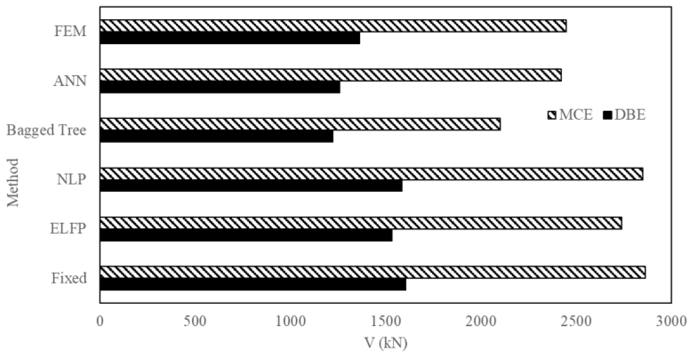
| Method | Vbase (kN) | Diff. from FEM | % Error | Vbase (kN) | Diff. from FEM | % Error |
| Fixed | 1604.24 | 240.99 | 17.68 | 2864.2 | 416.477 | 17.01 |
| ELFP | 1534.00 | 170.75 | 12.53 | 2738.77 | 291.05 | 11.89 |
| NLP | 1585.65 | 222.40 | 16.31 | 2851.38 | 403.66 | 16.49 |
| Bagged Tree | 1222.73 | 140.52 | 10.31 | 2100.55 | 347.17 | 14.18 |
| ANN * | 1257.53 | 105.72 | 7.75 | 2424.01 | 23.71 | 0.96 |
| FEM (reference) | 1363.25 | - | - | 2447.72 | - | - |
| 10%/50 yr (DBE) | 2%/50 yr (MCE) | |||||
|---|---|---|---|---|---|---|
| Method | MIDR (%) | Diff. from FEM | % Error | MIDR (%) | Diff. from FEM | % Error |
| Fixed | 1.48 | 0.20 | 15.63 | 2.64 | 0.22 | 9.09 |
| ELFP | 1.42 | 0.14 | 10.94 | 2.53 | 0.11 | 4.54 |
| NLP | 1.46 | 0.18 | 14.10 | 2.63 | 0.21 | 8.68 |
| Bagged Tree | 0.70 | 0.58 | 45.31 | 1.33 | 1.09 | 45.04 |
| ANN * | 1.25 | 0.03 | 2.34 | 2.39 | 0.03 | 1.23 |
| FEM (reference) | 1.28 | - | - | 2.42 | - | - |
Disclaimer/Publisher’s Note: The statements, opinions and data contained in all publications are solely those of the individual author(s) and contributor(s) and not of MDPI and/or the editor(s). MDPI and/or the editor(s) disclaim responsibility for any injury to people or property resulting from any ideas, methods, instructions or products referred to in the content. |
© 2023 by the authors. Licensee MDPI, Basel, Switzerland. This article is an open access article distributed under the terms and conditions of the Creative Commons Attribution (CC BY) license (https://creativecommons.org/licenses/by/4.0/).
Share and Cite
Ali, T.; Eldin, M.N.; Haider, W. The Effect of Soil-Structure Interaction on the Seismic Response of Structures Using Machine Learning, Finite Element Modeling and ASCE 7-16 Methods. Sensors 2023, 23, 2047. https://doi.org/10.3390/s23042047
Ali T, Eldin MN, Haider W. The Effect of Soil-Structure Interaction on the Seismic Response of Structures Using Machine Learning, Finite Element Modeling and ASCE 7-16 Methods. Sensors. 2023; 23(4):2047. https://doi.org/10.3390/s23042047
Chicago/Turabian StyleAli, Tabish, Mohamed Nour Eldin, and Waseem Haider. 2023. "The Effect of Soil-Structure Interaction on the Seismic Response of Structures Using Machine Learning, Finite Element Modeling and ASCE 7-16 Methods" Sensors 23, no. 4: 2047. https://doi.org/10.3390/s23042047
APA StyleAli, T., Eldin, M. N., & Haider, W. (2023). The Effect of Soil-Structure Interaction on the Seismic Response of Structures Using Machine Learning, Finite Element Modeling and ASCE 7-16 Methods. Sensors, 23(4), 2047. https://doi.org/10.3390/s23042047