


Weakly Supervised 2D Pose Adaptation and Body Part Segmentation for Concealed Object Detection †

Abstract
:1. Introduction
- We propose two methods for adapting an RGB pretrained pose detector to estimate accurate 2D poses in backscatter images, including a weakly supervised 3D–2D pose correction network that is optimized without ground-truth (GT) 2D or 3D pose annotations. Our proposed 2D pose refinement significantly improves the correctness of 2D poses in backscatter images.
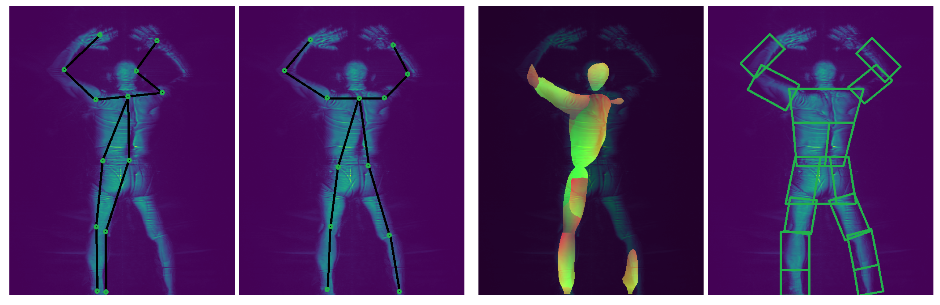
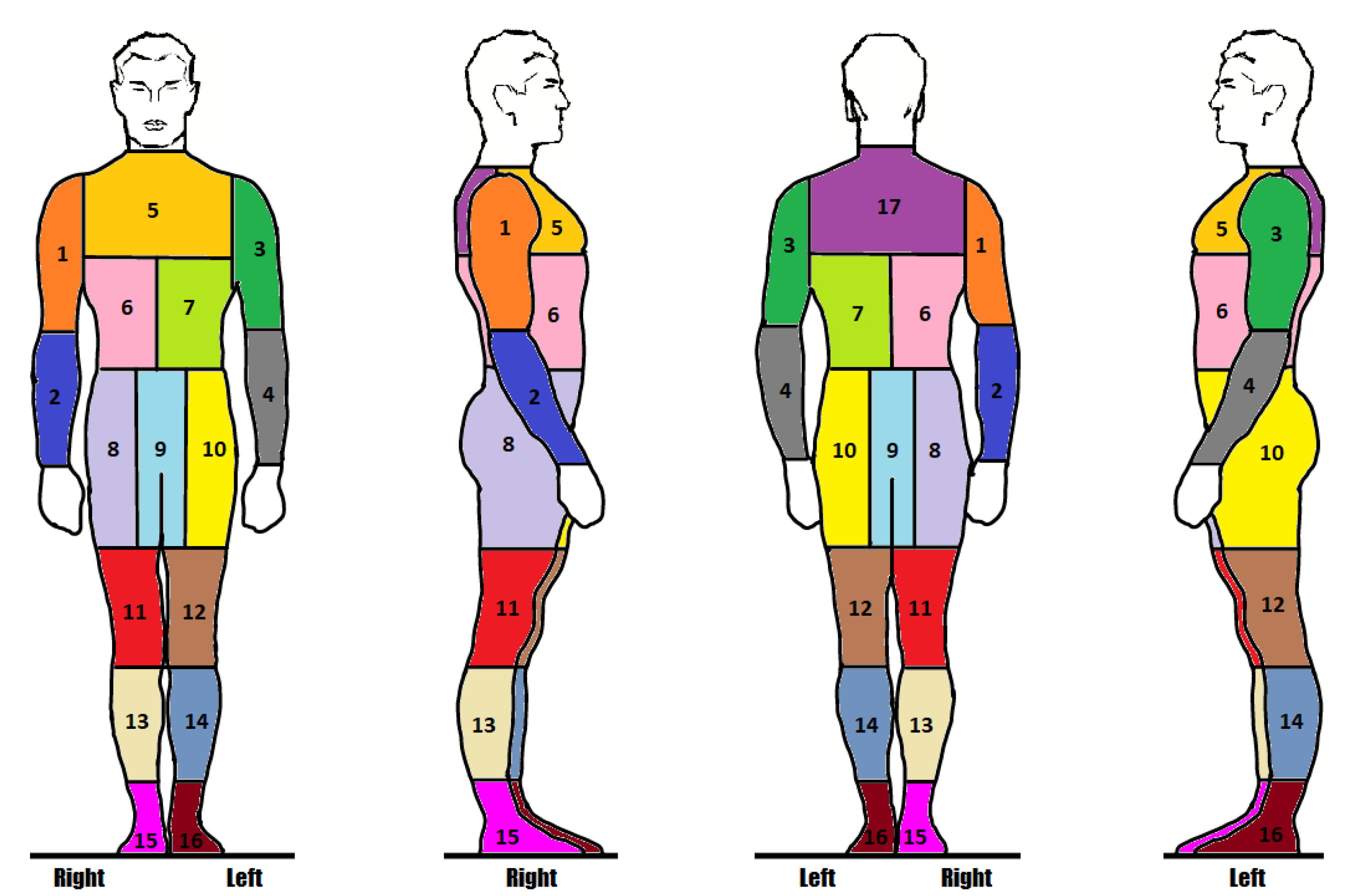
- We introduce an unsupervised procedure for segmenting human body parts in MWS images by estimating bounding polygons for each body part using keypoints of refined 2D poses. Our heuristic approach is motivated by the absence of body part annotations in the dataset and is effective at segmenting all body parts of a person in images captured from different viewpoints.
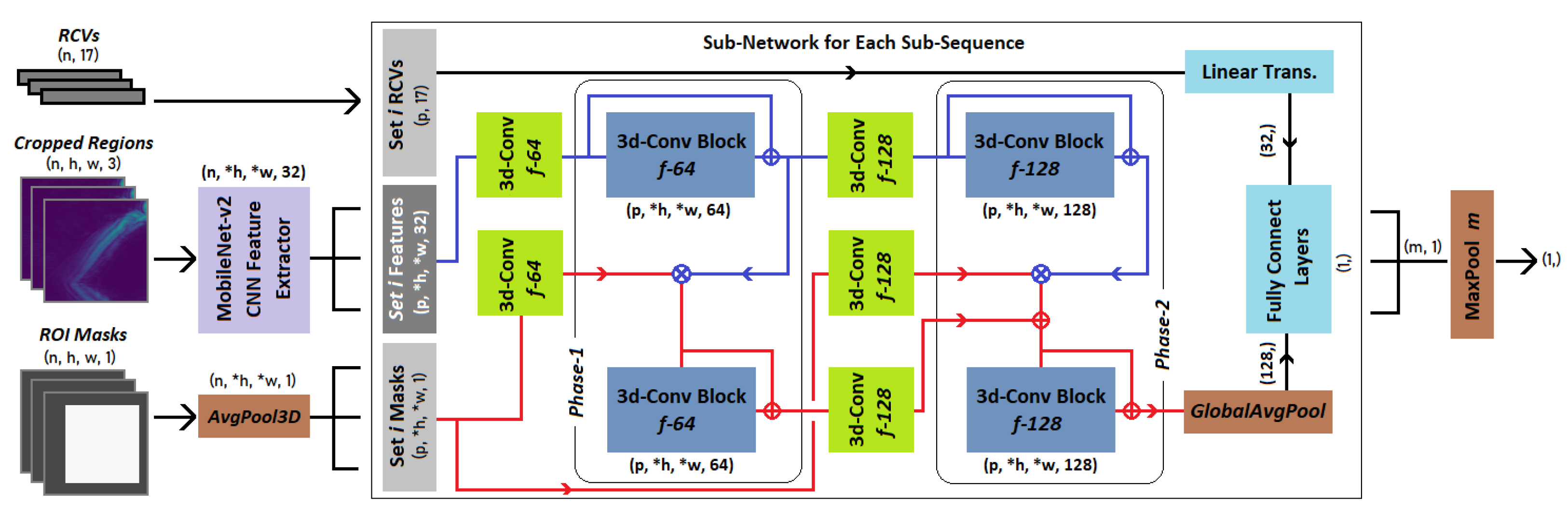
- We then propose a weakly supervised, ROI-attentive, dual-chain CNN classifier that detects anomalies given multi-view images of a cropped body part. Our anomaly detection network processes segmented images, their region of interest (ROI) masks, and derived region composite vectors (RCV) to decide if a detected anomaly should be attributed to a given body part. This ensures the network not only detects anomalies but also learns to associate anomalies with affected body parts, ultimately leading to more precise detection.
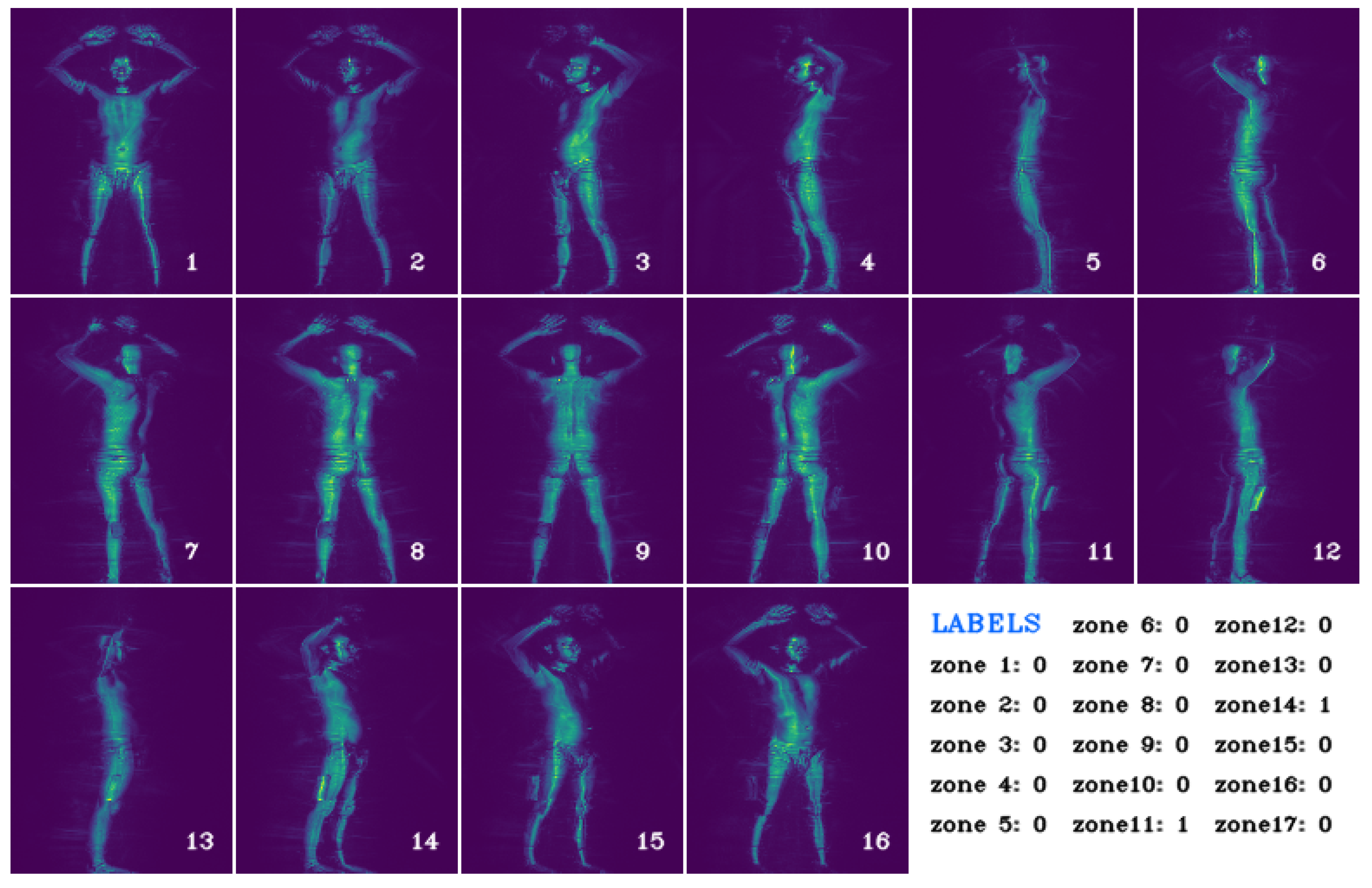
TSA Passenger Screening Dataset
2. Related Work
3. Method
3.1. Unsupervised Body Part Segmentation from 2D Poses
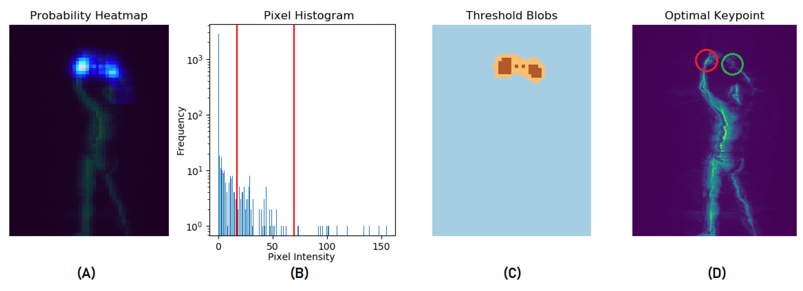
3.1.1. Keypoint Selection from HPE Confidence Maps
3.1.2. Multi-View Coherent Pose Optimization
| Algorithm 1 Per Keypoint RANSAC Bundle Adjustment | |
| Input: | ▹ 2D pixel positions of keypoint in each frame |
| Output: | ▹ 2D pixel positions of keypoint in each frame after bundle adjustment |
| 1: , | |
| 2: while do | ▹ iterate over subset of keypoints for 3D bundle adjustment |
| 3: | ▹ randomly selected subset, 1 every 4 consecutive frames |
| 4: | ▹ 3D point is regressed from R via least squares optimization |
| 5: | ▹ 2D positions after projecting to each frame |
| 6: | ▹ note inlier points based on Euclidean dist. between P & |
| 7: if then | |
| 8: | ▹ retain the largest inlier set |
| 9: end if | |
| 10: end while | |
| 11: | ▹ least squares bundle adjusted 3D point regressed from I 2D points |
| 12: | ▹ final 2D positions after projecting to each frame |
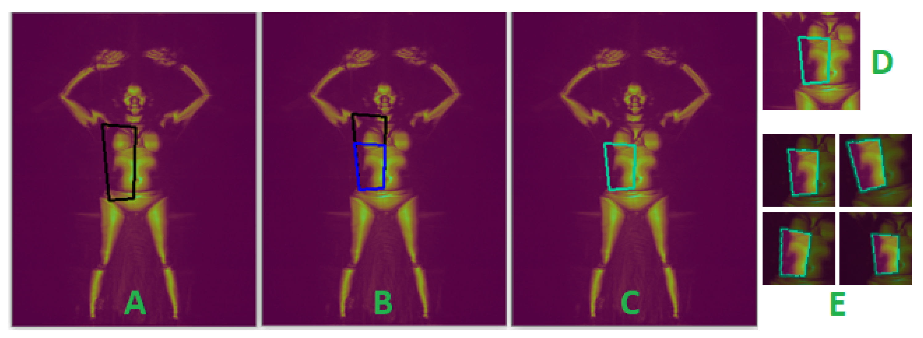
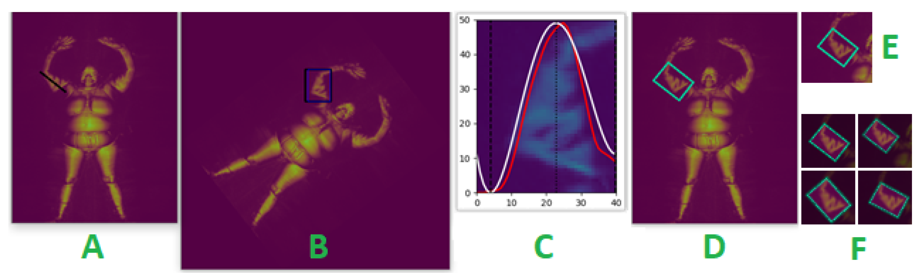
3.1.3. Estimating Bounding Polygons for Body Segmentation
Limb Body Part Segmentation
Torso Body Part Segmentation
3.2. RaadNet: ROI Attentive Anomaly Detection Network
Training and Inference with RaadNet Ensemble Classifiers
3.3. Extension: Learning Local Optimal 2D Pose Correction
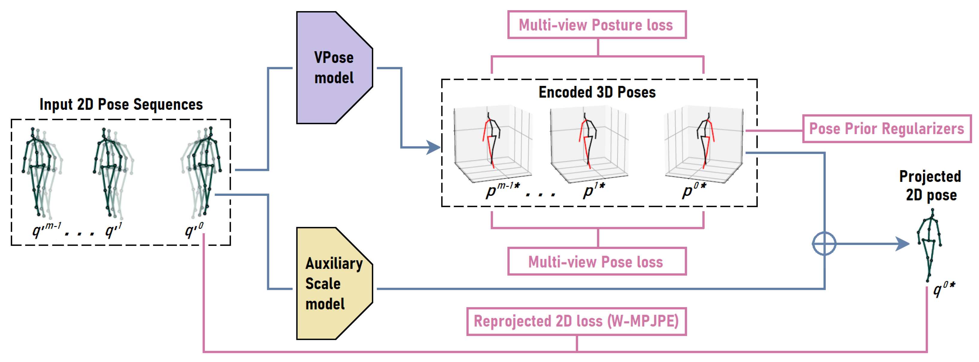
3.3.1. Weakly Supervised 3D to 2D Pose Correction Network
3.3.2. Weakly Supervised Loss Terms
Reprojected 2D Loss (R2D)
Multi-View Pose Consistency Loss
Multi-View Posture Consistency Loss
3.3.3. 3D Pose Prior Regularizers
Bone Proportion Constraint (BPC)
Joint Mobility Constraint (JMC)
4. Results
4.1. Evaluation of 2D Pose Refinement for MWS Images
4.2. Concealed Item Detection with RaadNet
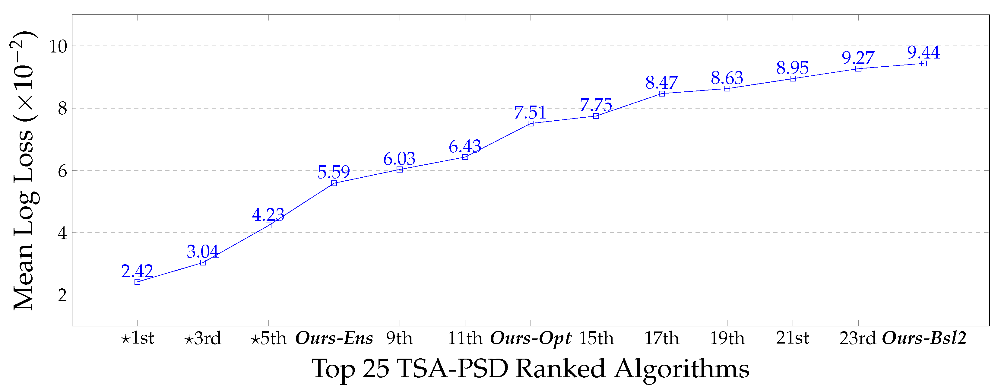
4.3. Comparison to TSA-PSD Proprietary Classifiers
5. Conclusions
Author Contributions
Funding
Informed Consent Statement
Data Availability Statement
Conflicts of Interest
Abbreviations
| HIPAA | Health Insurance Portability and Accountability Act |
| TSA | Transport Security Administration |
| TSA-PSD | Transport Security Administration Passenger Screening Challenge Dataset |
| HD-AIT | High Definition-Advanced Imaging Technology system |
| MWS | Millimeter Wave Scan images |
| H36M | Human3.6m 3D pose dataset |
| SOTA | State of the Art |
| ROI | Region of Interest |
| RCV | Region Composite Vector |
| CNN | Convolutional Neural Network |
| FCN | Fully Connected Network |
| CBI | Cropped Body part Image |
| GT | Ground Truth |
| RaadNet | ROI Attentive Anomaly Detection Network |
| W-MPJPE | Weighted Mean Per Joint Position Error |
| VPose | VideoPose3D Estimator Network |
| ICPR | International Conference on Pattern Recognition |
| NSF | National Science Foundation |
References
- Güler, R.A.; Trigeorgis, G.; Antonakos, E.; Snape, P.; Zafeiriou, S.; Kokkinos, I. DenseReg: Fully Convolutional Dense Shape Regression In-the-Wild. In Proceeding of the 2017 IEEE Conference on Computer Vision and Pattern Recognition (CVPR), Honolulu, HI, USA, 21–26 July 2017; pp. 2614–2623. [Google Scholar]
- Sun, K.; Xiao, B.; Liu, D.; Wang, J. Deep High-Resolution Representation Learning for Human Pose Estimation. arXiv 2019, arXiv:1902.09212. [Google Scholar]
- Amadi, L.; Agam, G. 2D-Pose Based Human Body Segmentation for Weakly-Supervised Concealed Object Detection in Backscatter Millimeter-Wave Images. In Proceedings of the 26th International Conference of Pattern Recognition Systems (T-CAP @ ICPR 2022), Montreal, QC, Canada, 21–25 August 2022. [Google Scholar]
- Amadi, L.; Agam, G. Multi-view Posture Analysis for Semi-Supervised 3D Monocular Pose Estimation. In Proceedings of the CVPR, Vancouver, BC, Canada, 18–22 June 2023. [Google Scholar]
- Amadi, L.; Agam, G. Boosting the Performance of Weakly-Supervised 3D Human Pose Estimators with Pose Prior Regularizers. In Proceedings of the ICIP, Bordeaux, France, 16–19 October 2022. [Google Scholar]
- TSA. Passenger Screening Challenge Dataset; U.S. Transportation Security Administration (TSA): Springfield, VA, USA, 2017. Available online: https://www.kaggle.com/competitions/passenger-screening-algorithm-challenge/data (accessed on 3 November 2018).
- Han, J.; Zhang, D.; Hu, X.; Guo, L.; Ren, J.; Wu, F. Background Prior-Based Salient Object Detection via Deep Reconstruction Residual. IEEE Trans. Circuits Syst. Video Technol. 2015, 25, 1309–1321. [Google Scholar]
- Cheng, G.; Han, J.; Guo, L.; Liu, T. Learning coarse-to-fine sparselets for efficient object detection and scene classification. In Proceedings of the 2015 IEEE Conference on Computer Vision and Pattern Recognition (CVPR), Boston, MA, USA, 7–12 June 2015; pp. 1173–1181. [Google Scholar]
- Li, J.; Xia, C.; Chen, X. A Benchmark Dataset and Saliency-Guided Stacked Autoencoders for Video-Based Salient Object Detection. IEEE Trans. Image Process. 2016, 27, 349–364. [Google Scholar] [CrossRef] [PubMed]
- Shin, H.C.; Orton, M.; Collins, D.J.; Doran, S.J.; Leach, M.O. Stacked Autoencoders for Unsupervised Feature Learning and Multiple Organ Detection in a Pilot Study Using 4D Patient Data. IEEE Trans. Pattern Anal. Mach. Intell. 2013, 35, 1930–1943. [Google Scholar] [CrossRef] [PubMed]
- Yan, K.; Li, C.; Wang, X.; Li, A.; Yuan, Y.; Kim, J.; Feng, D.D.F. Adaptive background search and foreground estimation for saliency detection via comprehensive autoencoder. In Proceedings of the 2016 IEEE International Conference on Image Processing (ICIP), Phoenix, AZ, USA, 25–28 September 2016; pp. 2767–2771. [Google Scholar] [CrossRef]
- Ronneberger, O.; Fischer, P.; Brox, T. U-Net: Convolutional Networks for Biomedical Image Segmentation. In Proceedings of the Computer Vision and Pattern Recognition (CVPR), Boston, MA, USA, 7–12 June 2015. [Google Scholar]
- He, K.; Gkioxari, G.; Dollár, P.; Girshick, R. Mask R-CNN. In Proceedings of the Computer Vision and Pattern Recognition (CVPR), Salt Lake City, UT, USA, 18–23 June 2018. [Google Scholar]
- Maqueda, I.G.; de la Blanca, N.P.; Molina, R.; Katsaggelos, A.K. Fast millimeter wave threat detection algorithm. In Proceedings of the 2015 23rd European Signal Processing Conference (EUSIPCO), Nice, France, 31 August–4 September 2015; pp. 599–603. [Google Scholar]
- Riffo, V.; Mery, D. Automated Detection of Threat Objects Using Adapted Implicit Shape Model. IEEE Trans. Syst. Man Cybern. Syst. 2016, 46, 472–482. [Google Scholar] [CrossRef]
- Ajami, M.; Lang, B. Using RGB-D Sensors for the Detection of Unattended Luggage. In Proceedings of the 7th International Conference on Imaging for Crime Detection and Prevention (ICDP 2016), Madrid, Spain, 23–25 November 2016. [Google Scholar]
- Thangavel, S. Hidden object detection for classification of threat. In Proceedings of the 2017 4th International Conference on Advanced Computing and Communication Systems (ICACCS), Coimbatore, India, 6–7 January 2017; pp. 1–7. [Google Scholar] [CrossRef]
- Bhattacharyya, A.; Lind, C.H. Threat Detection in TSA Scans Using AlexNet; University of California: San Diego, CA, USA, 2018. [Google Scholar]
- Guimaraes, A.A.R.; Tofighi, G. Detecting Zones and Threat on 3D Body for Security in Airports using Deep Machine Learning. arXiv 2018, arXiv:1802.00565. [Google Scholar]
- Cao, Z.; Simon, T.; Wei, S.E.; Sheikh, Y. Realtime Multi-Person 2D Pose Estimation using Part Affinity Fields. In Proceedings of the Computer Vision and Pattern Recognition (CVPR), Honolulu, HI, USA, 21–26 July 2017. [Google Scholar]
- Toshev, A.; Szegedy, C. DeepPose: Human Pose Estimation via Deep Neural Networks. In Proceedings of the 2014 IEEE Conference on Computer Vision and Pattern Recognition, Columbus, OH, USA, 23–28 June 2014; pp. 1653–1660. [Google Scholar]
- Newell, A.; Yang, K.; Deng, J. Stacked Hourglass Networks for Human Pose Estimation. In Proceedings of the ECCV, Amsterdam, The Netherlands, 11–14 October 2016. [Google Scholar]
- Chen, Y.; Wang, Z.; Peng, Y.; Zhang, Z.; Yu, G.; Sun, J. Cascaded Pyramid Network for Multi-person Pose Estimation. In Proceedings of the 2017 IEEE/CVF Conference on Computer Vision and Pattern Recognition, Honolulu, HI, USA, 21–26 July 2017; pp. 7103–7112. [Google Scholar]
- Hidalgo, G.; Raaj, Y.; Idrees, H.; Xiang, D.; Joo, H.; Simon, T.; Sheikh, Y. Single-Network Whole-Body Pose Estimation. In Proceedings of the 2019 IEEE/CVF International Conference on Computer Vision (ICCV), Seoul, Republic of Korea, 27 October–2 November 2019; pp. 6981–6990. [Google Scholar]
- Xia, F.; Wang, P.; Chen, X.; Yuille, A.L. Joint Multi-person Pose Estimation and Semantic Part Segmentation. In Proceedings of the 2017 IEEE Conference on Computer Vision and Pattern Recognition (CVPR), Honolulu, HI, USA, 21–26 July 2017; pp. 6080–6089. [Google Scholar]
- Fang, H.; Lu, G.; Fang, X.; Xie, J.; Tai, Y.W.; Lu, C. Weakly and Semi Supervised Human Body Part Parsing via Pose-Guided Knowledge Transfer. In Proceedings of the 2018 IEEE/CVF Conference on Computer Vision and Pattern Recognition, Salt Lake City, UT, USA, 18–23 June 2018; pp. 70–78. [Google Scholar]
- Saviolo, A.; Bonotto, M.; Evangelista, D.; Imperoli, M.; Menegatti, E.; Pretto, A. Learning to Segment Human Body Parts with Synthetically Trained Deep Convolutional Networks. In Proceedings of the 16th International Conference IAS-16, Singapore, 22–25 June 2021. [Google Scholar]
- Gong, K.; Liang, X.; Li, Y.; Chen, Y.; Yang, M.; Lin, L. Instance-level Human Parsing via Part Grouping Network. arXiv 2018, arXiv:1808.00157. [Google Scholar]
- Yang, L.; Song, Q.; Wang, Z.; Jiang, M. Parsing R-CNN for Instance-Level Human Analysis. In Proceedings of the 2019 IEEE/CVF Conference on Computer Vision and Pattern Recognition (CVPR), Long Beach, CA, USA, 15–20 June 2019; pp. 364–373. [Google Scholar]
- Li, P.; Xu, Y.; Wei, Y.; Yang, Y. Self-Correction for Human Parsing. IEEE Trans. Pattern Anal. Mach. D 2022, 44, 3260–3271. [Google Scholar] [CrossRef]
- Lin, K.; Wang, L.; Luo, K.; Chen, Y.; Liu, Z.; Sun, M.T. Cross-Domain Complementary Learning Using Pose for Multi-Person Part Segmentation. IEEE Trans. Circuits Syst. Video Technol. 2020, 31, 1066–1078. [Google Scholar] [CrossRef]
- Hynes, A.; Czarnuch, S. Human Part Segmentation in Depth Images with Annotated Part Positions. Sensors 2018, 18, 1900. [Google Scholar] [CrossRef]
- Luo, Y.; Zheng, Z.; Zheng, L.; Guan, T.; Yu, J.; Yang, Y. Macro-Micro Adversarial Network for Human Parsing. In Proceedings of the ECCV, Munich, Germany, 8–14 September 2018. [Google Scholar]
- Zhang, S.H.; Li, R.; Dong, X.; Rosin, P.L.; Cai, Z.; Han, X.; Yang, D.; Huang, H.; Hu, S. Pose2Seg: Detection Free Human Instance Segmentation. In Proceedings of the 2019 IEEE/CVF Conference on Computer Vision and Pattern Recognition (CVPR), Long Beach, CA, USA, 15–20 June 2019; pp. 889–898. [Google Scholar]
- Gruosso, M.; Capece, N.; Erra, U. Human segmentation in surveillance video with deep learning. Multimed. Tools Appl. 2021, 80, 1175–1199. [Google Scholar] [CrossRef]
- Yaniv, Z. Random Sample Consensus ( RANSAC ) Algorithm, A Generic Implementation Release. Available online: http://www.yanivresearch.info/writtenMaterial/RANSAC.pdf (accessed on 1 December 2022).
- Lin, T.Y.; Maire, M.; Belongie, S.J.; Bourdev, L.D.; Girshick, R.B.; Hays, J.; Perona, P.; Ramanan, D.; Dollár, P.; Zitnick, C.L. Microsoft COCO: Common Objects in Context. In Proceedings of the ECCV, Zurich, Switzerland, 6–12 September 2014; Available online: http://cocodataset.org/#home (accessed on 1 December 2022).
- Zhang, J.; Hu, J. Image Segmentation Based on 2D Otsu Method with Histogram Analysis. In Proceedings of the 2008 International Conference on Computer Science and Software Engineering, Wuhan, China, 12–14 December 2008; Volume 6, pp. 105–108. [Google Scholar]
- Fioraio, N.; di Stefano, L. Joint Detection, Tracking and Mapping by Semantic Bundle Adjustment. In Proceedings of the 2013 IEEE Conference on Computer Vision and Pattern Recognition, Portland, OR, USA, 23–28 June 2013; pp. 1538–1545. [Google Scholar]
- Triggs, B.; McLauchlan, P.; Hartley, R.; Fitzgibbon, A. Bundle Adjustment—A Modern Synthesis. In Proceedings of the Workshop on Vision Algorithms, Corfu, Greece, 21–22 September 1999. [Google Scholar]
- Grisetti, G.; Guadagnino, T.; Aloise, I.; Colosi, M.; Corte, B.D.; Schlegel, D. Least Squares Optimization: From Theory to Practice. Robotics 2020, 9, 51. [Google Scholar] [CrossRef]
- Curtis, A.R.; Powell, M.J.D.; Reid, J.K. On the Estimation of Sparse Jacobian Matrices. IMA J. Appl. Math. 1974, 13, 117–119. [Google Scholar] [CrossRef]
- Sandler, M.; Howard, A.G.; Zhu, M.; Zhmoginov, A.; Chen, L.C. MobileNetV2: Inverted Residuals and Linear Bottlenecks. In Proceedings of the 2018 IEEE/CVF Conference on Computer Vision and Pattern Recognition, Salt Lake City, UT, USA, 18–23 June 2018; pp. 4510–4520. [Google Scholar]
- Deng, J.; Dong, W.; Socher, R.; Li, L.J.; Li, K.; Fei-Fei, L. ImageNet: A Large-Scale Hierarchical Image Database. In Proceedings of the CVPR09, Miami, FL, USA, 20–25 June 2009; Available online: http://image-net.org/index (accessed on 20 February 2018).
- Kingma, D.P.; Ba, J. Adam: A Method for Stochastic Optimization. arXiv 2014, arXiv:1412.6980. [Google Scholar]
- Pavllo, D.; Feichtenhofer, C.; Grangier, D.; Auli, M. 3D human pose estimation in video with temporal convolutions and semi-supervised training. In Proceedings of the Computer Vision and Pattern Recognition (CVPR), Long Beach, CA, USA, 15–20 June 2019. [Google Scholar]
- Ionescu, C.; Papava, D.; Olaru, V.; Sminchisescu, C. Human3.6M: Large Scale Datasets and Predictive Methods for 3D Human Sensing in Natural Environments. IEEE Trans. Pattern Anal. Mach. Intell. 2014, 36, 1325–1339. [Google Scholar] [CrossRef] [PubMed]
- Richer, P. Richer’s Average Human Proportions—7.5 Heads. Artistic Anatomy: The Great French Classic on Artistic Anatomy. Available online: https://www.proko.com/human-figure-proportions-average-richer (accessed on 10 August 2019).
- Hale, R.B. Hales’s Cranial Method for Human Proportions. Available online: https://www.proko.com/human-figure-proportions-cranium-unit-hale (accessed on 10 August 2019).
- Loomis, A. Loomis Idealistic Proportions. Available online: https://www.proko.com/human-figure-proportions-idealistic-loomis (accessed on 10 August 2019).


| mm | R.Sh | R.Eb | R.Wr | L.Sh | L.Eb | L.Wr | R.Hp | R.Ke | R.Ak | L.Hp | L.Ke | L.Ak | Avg. |
|---|---|---|---|---|---|---|---|---|---|---|---|---|---|
| Generic Pose | 115.7 | 191.5 | 119.1 | 100.4 | 173.4 | 117.6 | 88.49 | 115.3 | 137.3 | 79.91 | 105.8 | 134.5 | 123.2 |
| Confined Pose | 55.2 | 36.9 | 35.2 | 52.3 | 44.4 | 42.6 | 65.1 | 38.5 | 42.9 | 61.6 | 36.9 | 43.6 | 46.3 |
| Coherent Pose-1 | 40.2 | 32.5 | 19.9 | 38.1 | 31.4 | 23.6 | 82.8 | 38.9 | 22.4 | 78.1 | 35.8 | 21.0 | 38.7 |
| Coherent Pose-2 | 37.4 | 30.2 | 19.5 | 35.8 | 31.5 | 20.2 | 64.5 | 38.3 | 21.1 | 61.2 | 35.3 | 20.4 | 34.6 |
| Coherent Pose-3 | 35.6 | 28.0 | 17.1 | 35.2 | 17.5 | 17.3 | 61.8 | 36.0 | 20.2 | 61.2 | 35.1 | 20.6 | 32.1 |
| Body Part Anomaly Detection Methods | Validation Set | Test | |||||
|---|---|---|---|---|---|---|---|
| Avg.F1 ↑ | F1.Score ↑ | Precision ↑ | Recall ↑ | Accuracy ↑ | Logloss ↓ | Logloss ↓ | |
| FastNet (*) [14] | 0.8890 | - | - | - | - | - | - |
| AlexNet-1 (*) [18] | - | - | - | - | - | 0.0088 | - |
| AlexNet-2 (*) [19] | 0.9828 | - | - | - | - | - | 0.0913 |
| RaadNet + FixedSeg. [18] + Mask + RCV (Bsl-1) | 0.9761 | 0.9555 | 0.9628 | 0.9487 | 0.9723 | 0.0201 | 0.1384 |
| RaadNet + Unref.PoseSeg. + Mask + RCV (Bsl-2) | 0.9184 | 0.7526 | 0.8652 | 0.6659 | 0.9108 | 0.1282 | 0.1608 |
| Ours RaadNet + Co.PoseSeg. (Abl-1) | 0.9775 | 0.9581 | 0.9655 | 0.9505 | 0.9766 | 0.0143 | 0.0934 |
| Ours RaadNet + Co.PoseSeg. + Mask (Abl-2) | 0.9637 | 0.9540 | 0.9550 | 0.9531 | 0.9687 | 0.0131 | 0.0886 |
| Ours RaadNet + Co.PoseSeg. + Mask + RCV (Opt.) | 0.9859 | 0.9738 | 0.9941 | 0.9544 | 0.9946 | 0.0097 | 0.0751 |
Disclaimer/Publisher’s Note: The statements, opinions and data contained in all publications are solely those of the individual author(s) and contributor(s) and not of MDPI and/or the editor(s). MDPI and/or the editor(s) disclaim responsibility for any injury to people or property resulting from any ideas, methods, instructions or products referred to in the content. |
© 2023 by the authors. Licensee MDPI, Basel, Switzerland. This article is an open access article distributed under the terms and conditions of the Creative Commons Attribution (CC BY) license (https://creativecommons.org/licenses/by/4.0/).
Share and Cite
Amadi, L.; Agam, G. Weakly Supervised 2D Pose Adaptation and Body Part Segmentation for Concealed Object Detection. Sensors 2023, 23, 2005. https://doi.org/10.3390/s23042005
Amadi L, Agam G. Weakly Supervised 2D Pose Adaptation and Body Part Segmentation for Concealed Object Detection. Sensors. 2023; 23(4):2005. https://doi.org/10.3390/s23042005
Chicago/Turabian StyleAmadi, Lawrence, and Gady Agam. 2023. "Weakly Supervised 2D Pose Adaptation and Body Part Segmentation for Concealed Object Detection" Sensors 23, no. 4: 2005. https://doi.org/10.3390/s23042005
APA StyleAmadi, L., & Agam, G. (2023). Weakly Supervised 2D Pose Adaptation and Body Part Segmentation for Concealed Object Detection. Sensors, 23(4), 2005. https://doi.org/10.3390/s23042005