
A Low-Cost, Low-Power, Multisensory Device and Multivariable Time Series Prediction for Beehive Health Monitoring

 , ,
, , 
Abstract
1. Introduction
- (A)
- We present an open solution that is based on custom electronics, and we do not make use of ready platforms as in many published results. Platforms such as Arduino and Raspberry Pi facilitate experimentation and are widely used in literature on beehive-related technology, but ready platforms are generic and thus not optimal in terms of power consumption and cost. We need solutions that are power sufficient because we need to avoid the manual visits to remote locations and to be affordable so that automated monitoring of health status shifts from research to commercial applications. All details are available so that it can be reproduced and its cost is assessed.
- (B)
- We test sensor capabilities that are not the norm in commercial beehive supervision technology. Specifically, we test CO2 concentration and volatile compounds (TVOC) gas sensors, vibration sensors as well as a bee counter appended to typical measurements (specifically: weight, temperature, humidity, GPS coordinates, and timestamps of recording events). We design our board to sample all sensors simultaneously and create a multivariable time series that is transmitted to a cloud server.
- (C)
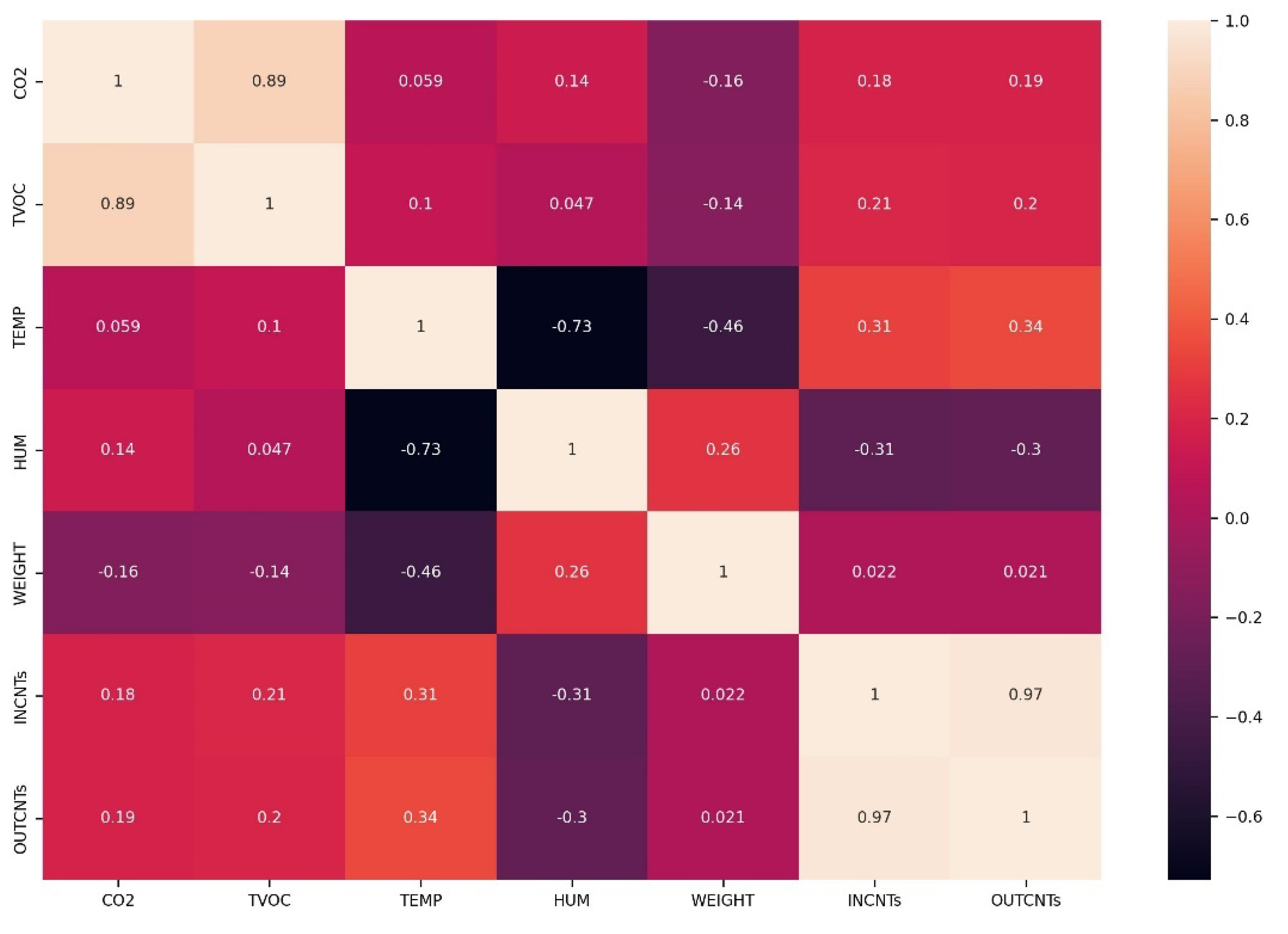
- We investigate and quantify how the prediction of a single variable, e.g., CO2 concentration, is affected by the inclusion of additional regressors (e.g., temperature, humidity). The multivariable time series is used to run forecasting models and risk assessments [28,29,30,31], issue warnings and alert signals and make historical analysis with applied confidence intervals.
2. Materials and Methods
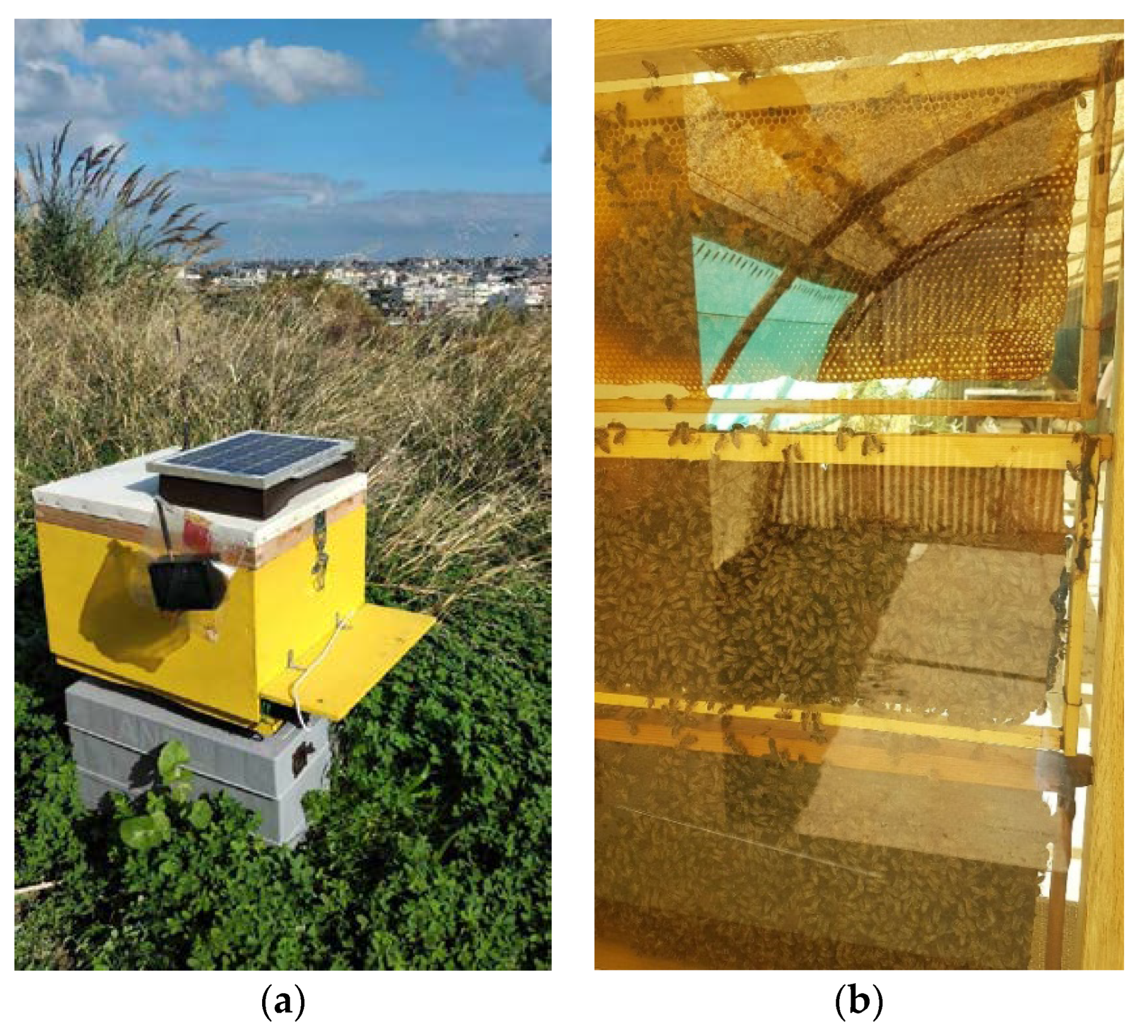
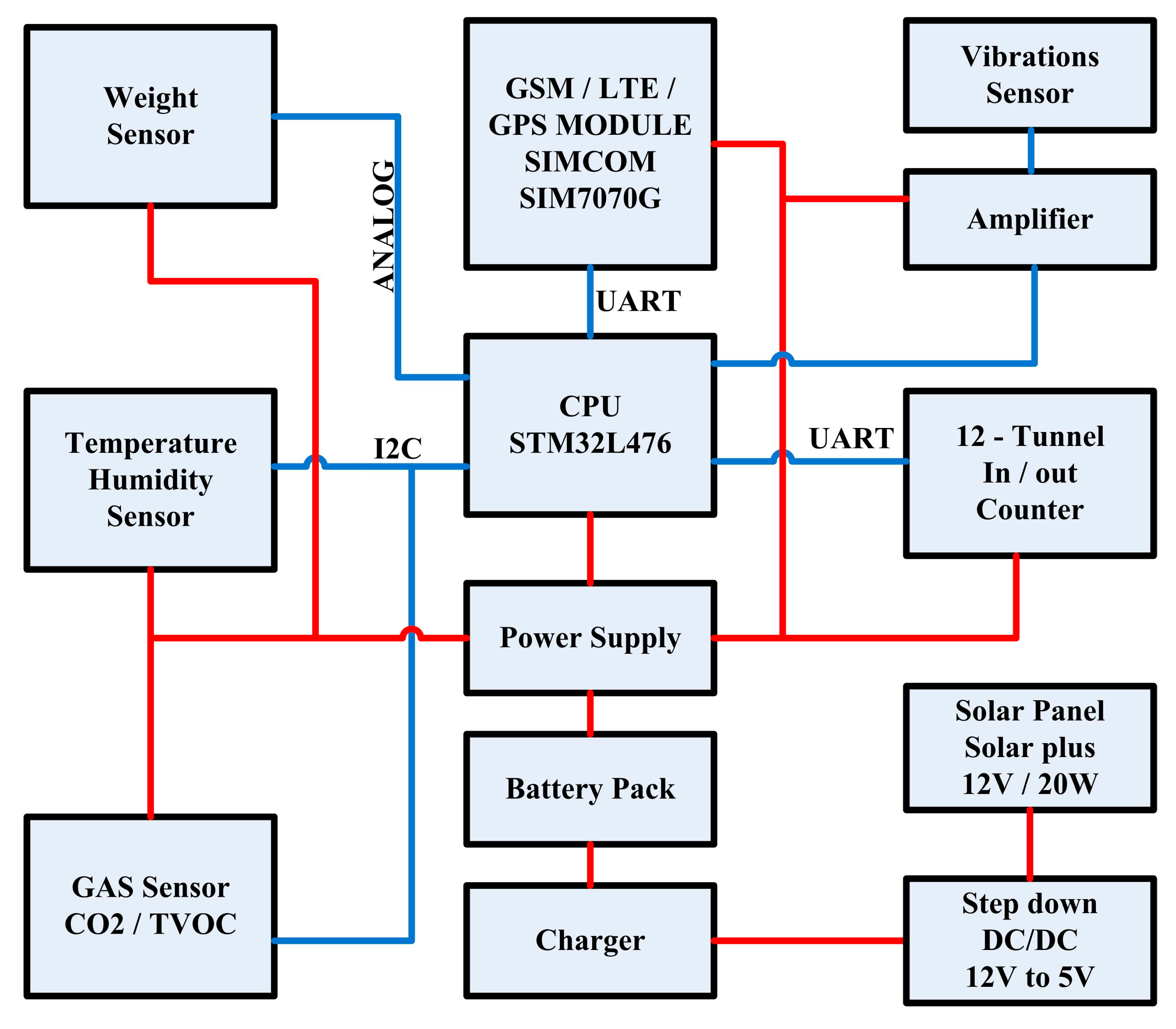
2.1. The Components of the Multisensory Recorder
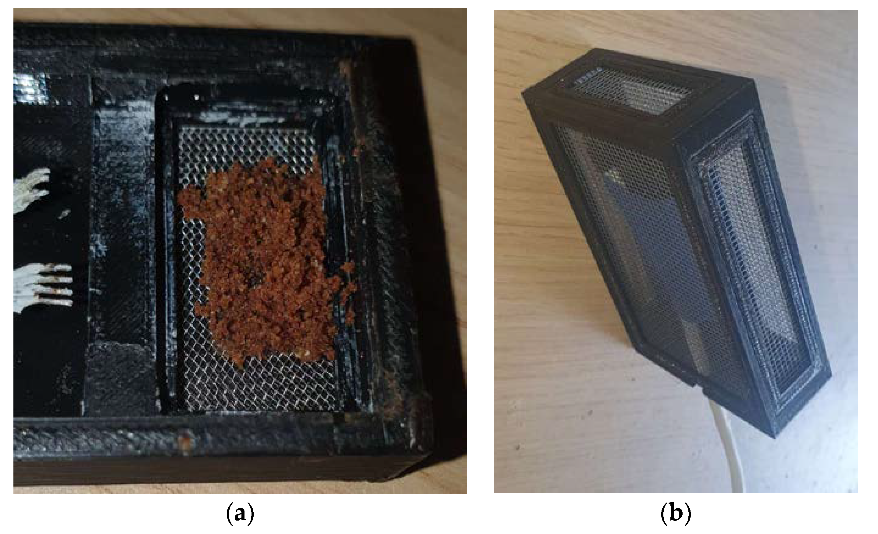
2.1.1. The Gas Sensor
CO2 Concentration
TVOC Concentration
2.1.2. Vibrations
2.1.3. Temperature and Humidity
Temperature
Humidity
2.1.4. The Weight Sensor
2.1.5. The Bee Counter
2.1.6. Power Supply
2.2. Programming
2.3. Prediction Models
3. Results
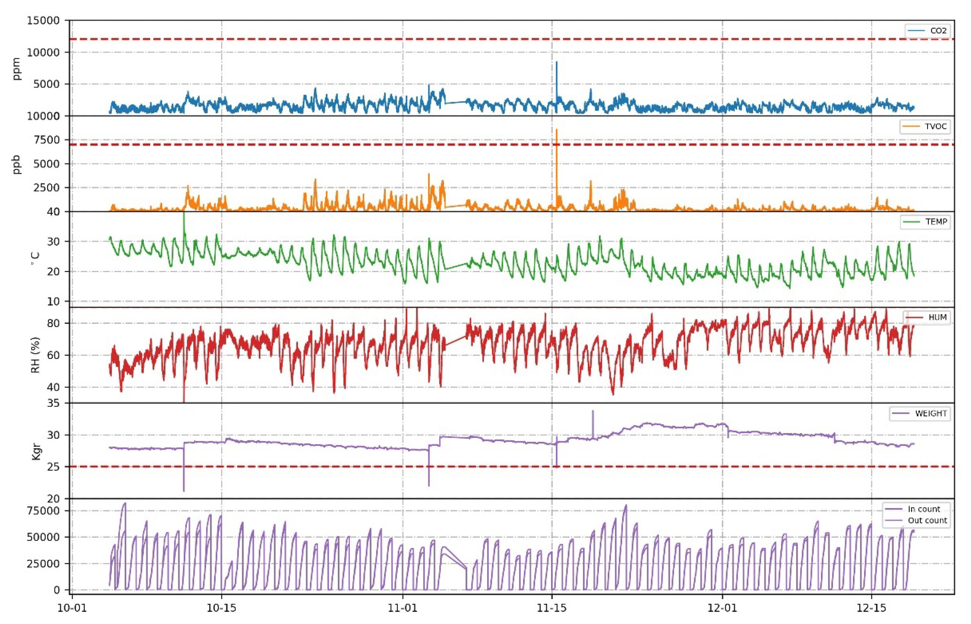
3.1. The Signals
- (1)
- Time stamp of events. Measurements taken every 5 min on a 24/7 basis, for all sensors simultaneously.
- (2)
- GPS coordinates that are used to localize the beehive on a map, on the server’s part and as a theft prevention measure.
- (3)
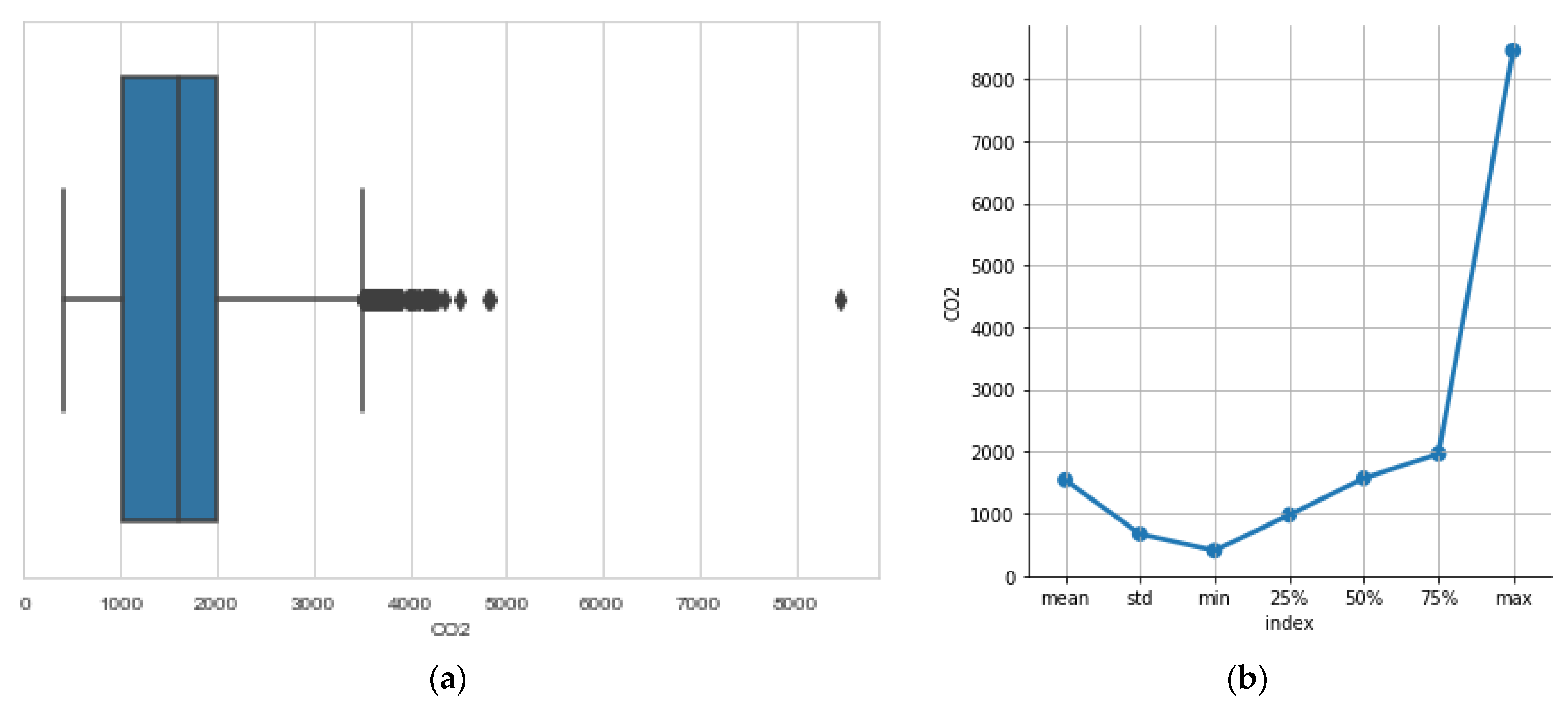
- CO2 concentration inside the hive (parts per million—ppm).
- (4)
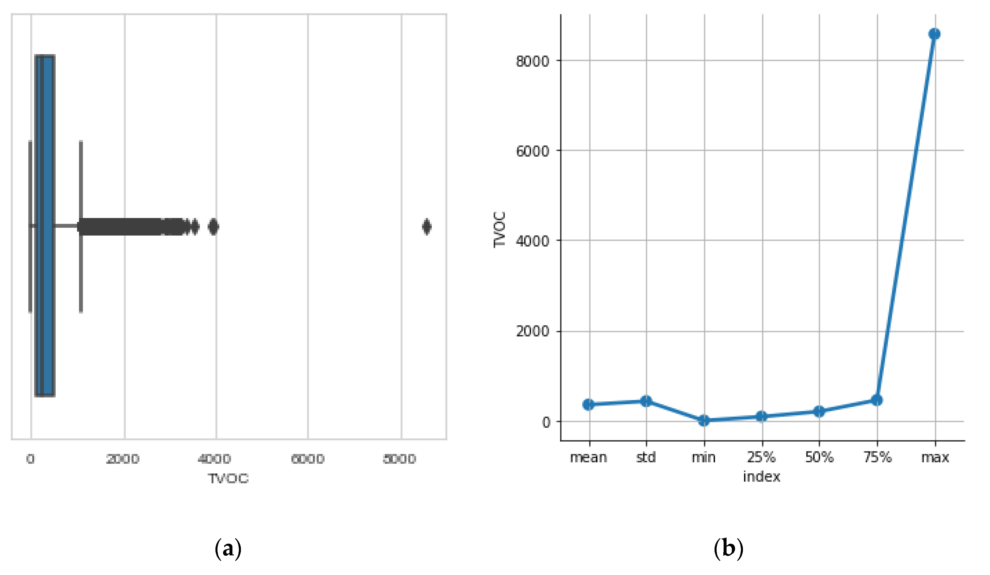
- Total volatile organic compounds concentration TVOC inside the hive (parts per billion—ppb).
- (5)
- Temperature inside the beehive (°C).
- (6)
- Relative humidity in the interior of the beehive (% RH).
- (7)
- Weight (Kgr) of the beehive (including honey, bees and pollen).
- (8)
- Incoming bee counts.
- (9)
- Outgoing bee counts.
- (10)
- Five sec vibrations recording from which features are extracted (e.g., energy in specific frequencies that are deemed important e.g., piping, tooting, tremble, whooping signals).
- (11)
- Quality of signal communication (used for telemetry at the server part).
- (12)
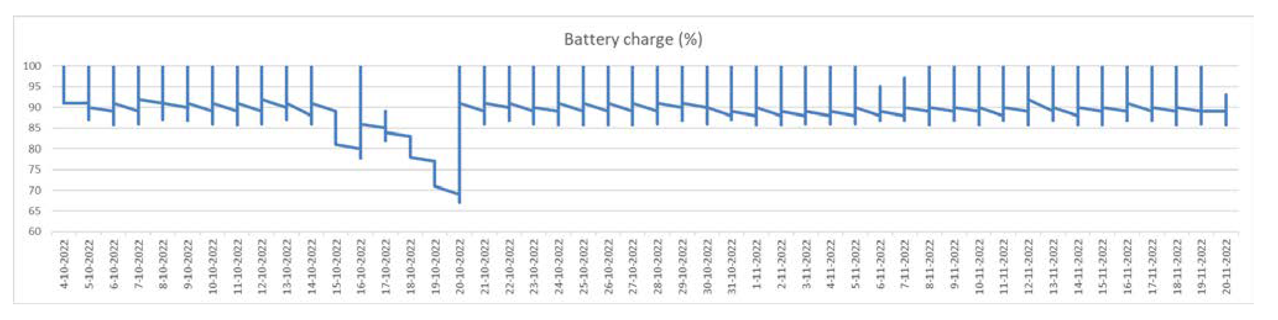
- Battery charge level (used for telemetry at the server part).
3.2. The CO2 Concentration
3.3. The TVOC Concentration
3.4. The Weight
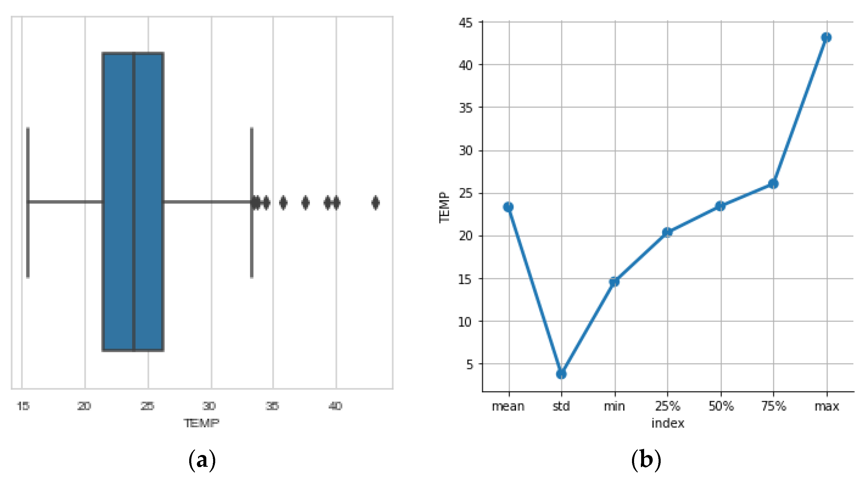
3.5. The Temperature
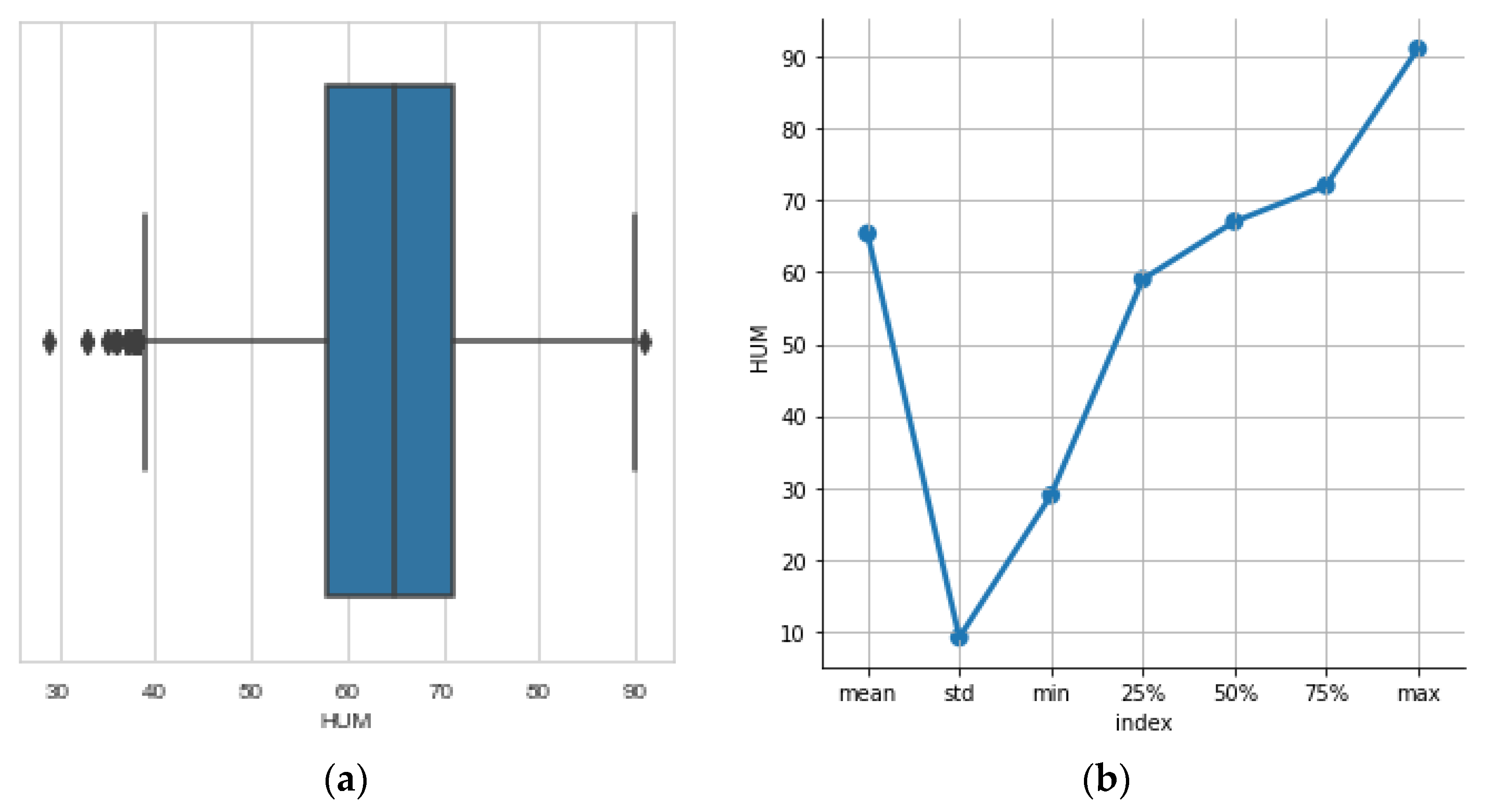
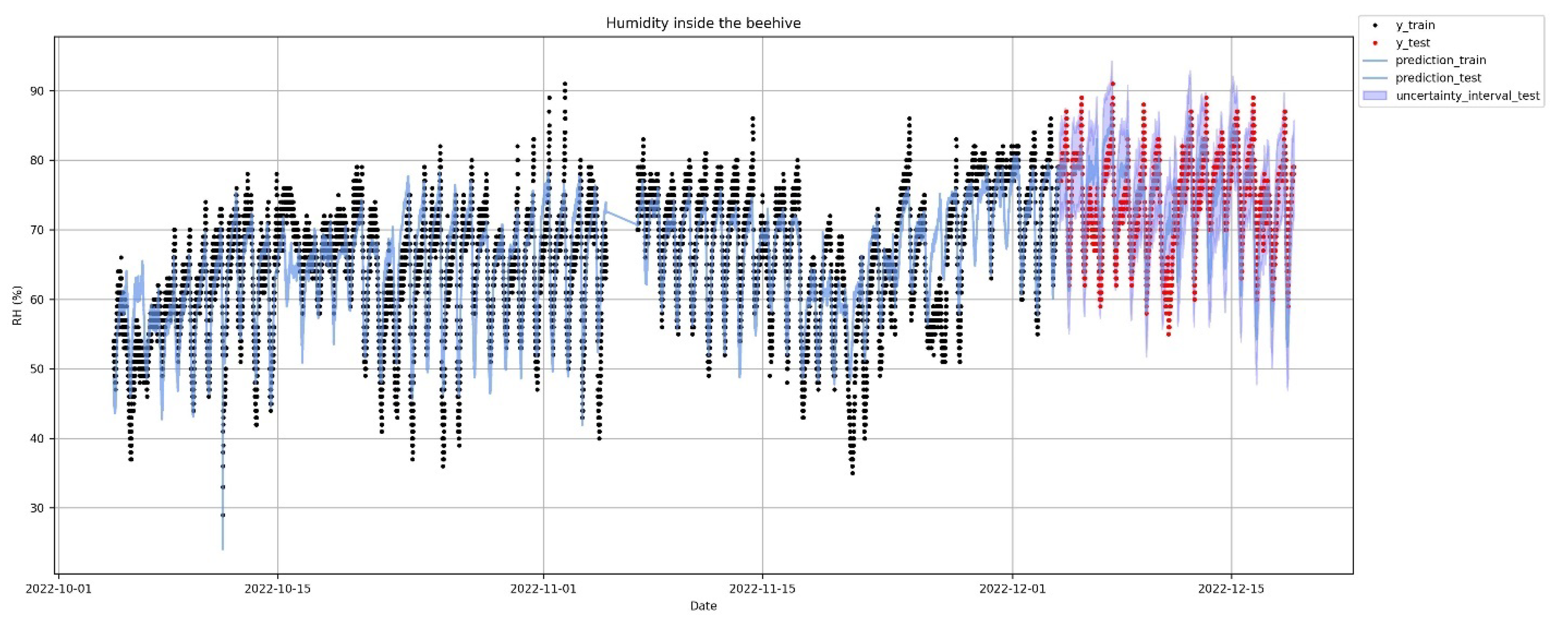
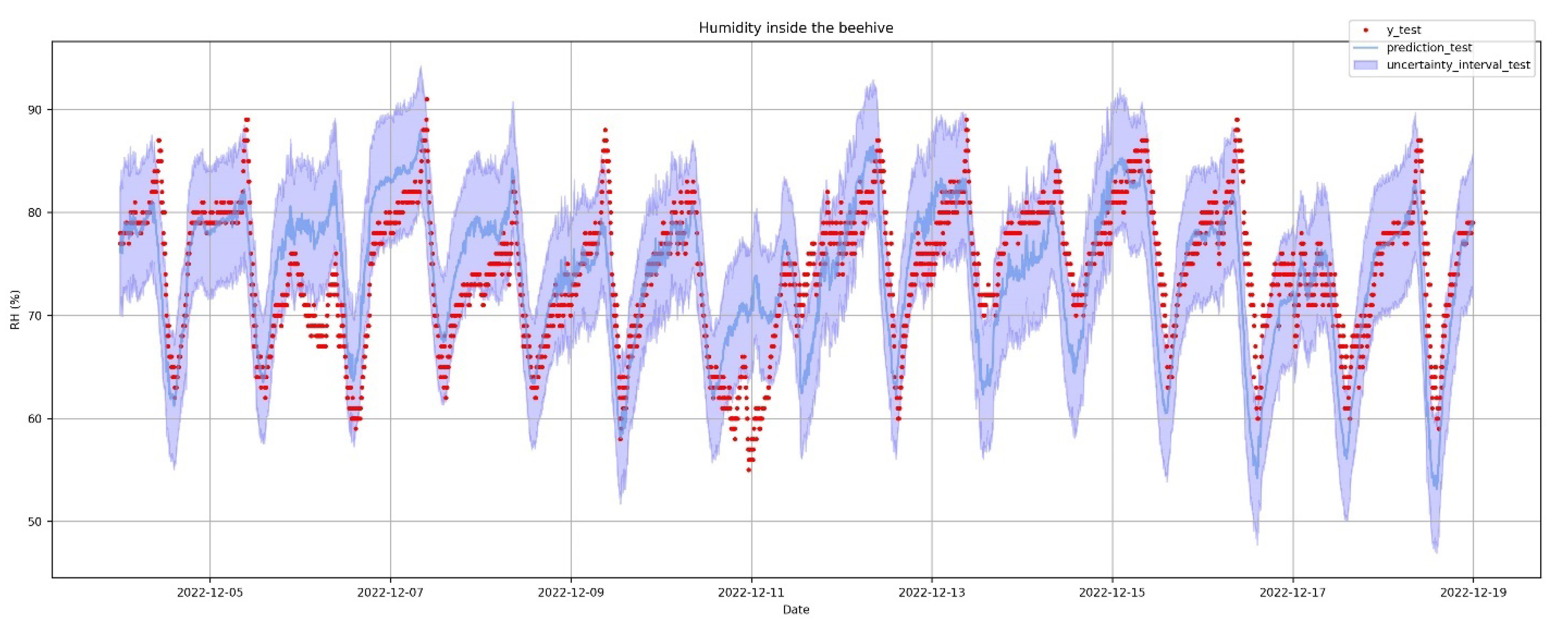
3.6. The Humidity
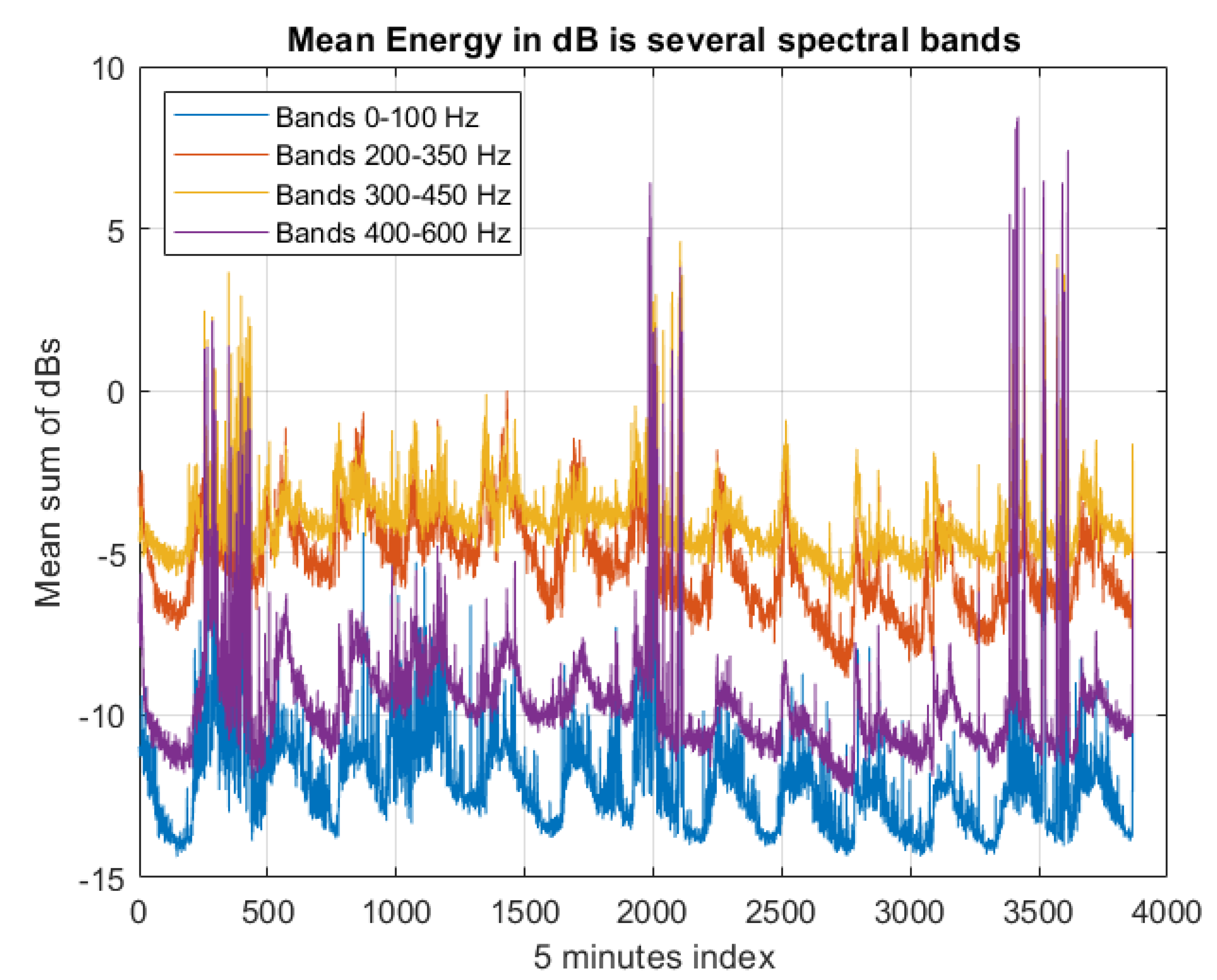
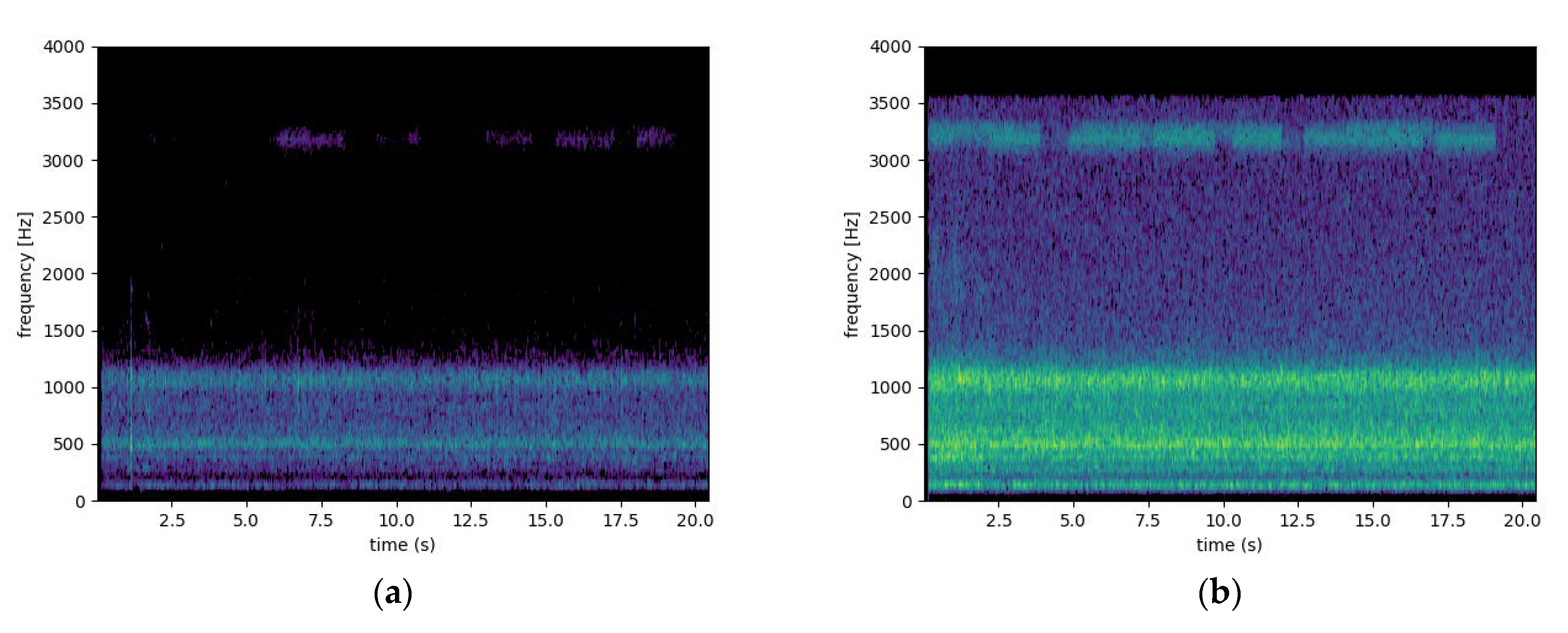
3.7. The Vibrations Sensor
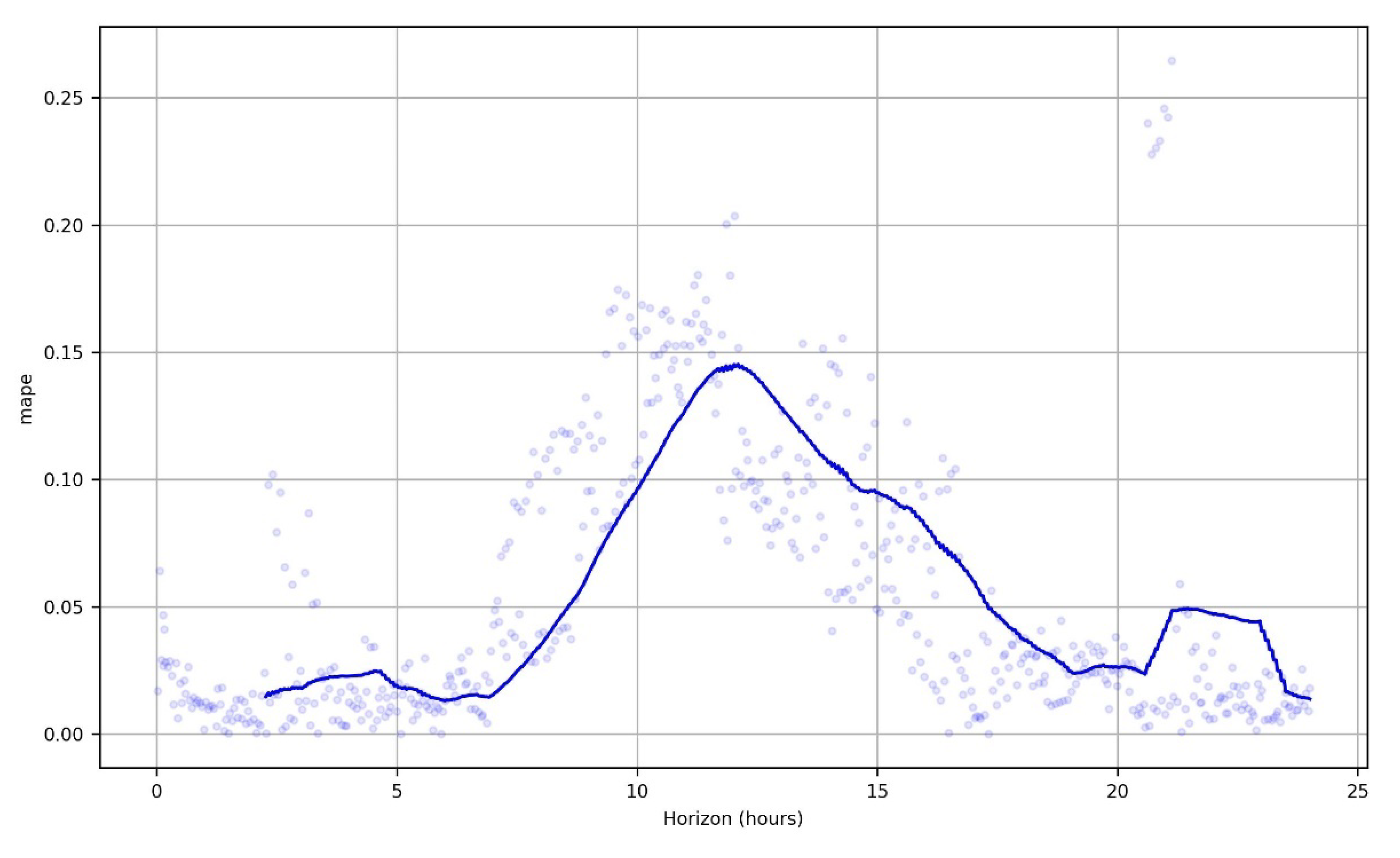
3.8. Error Measurements of Prediction Models
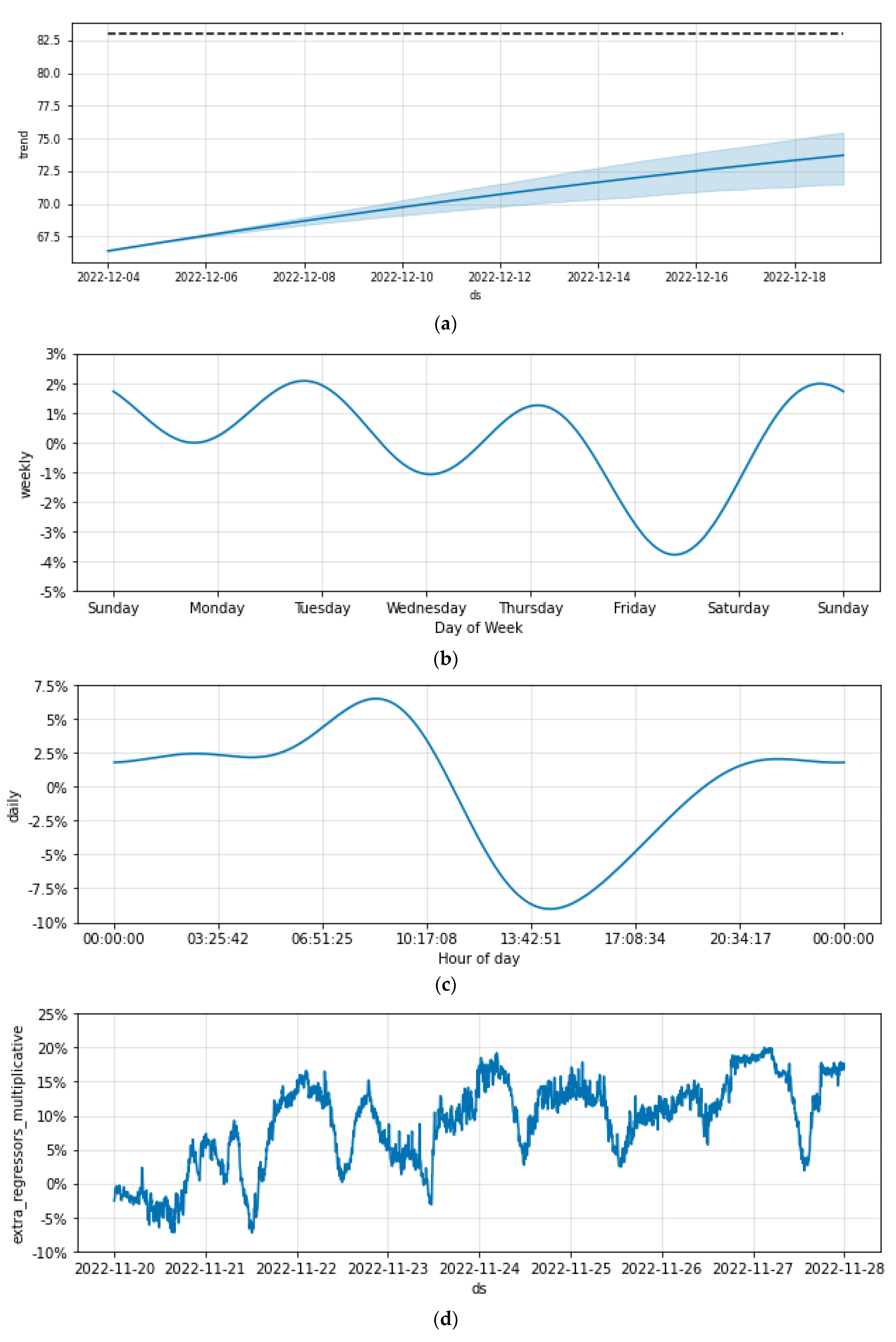
3.8.1. Prophet: Additive Regression Model
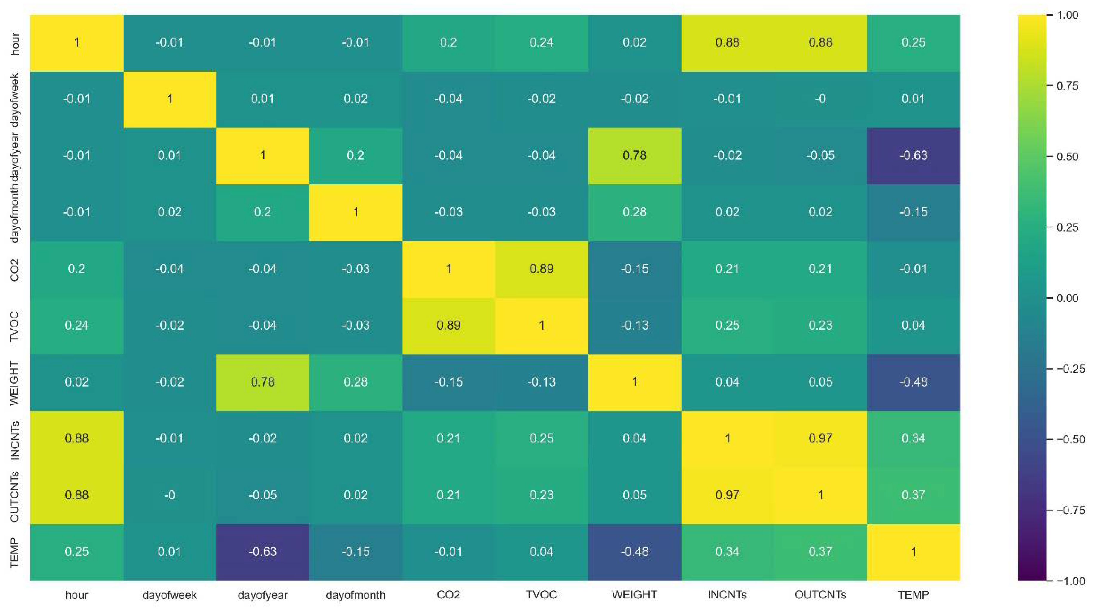
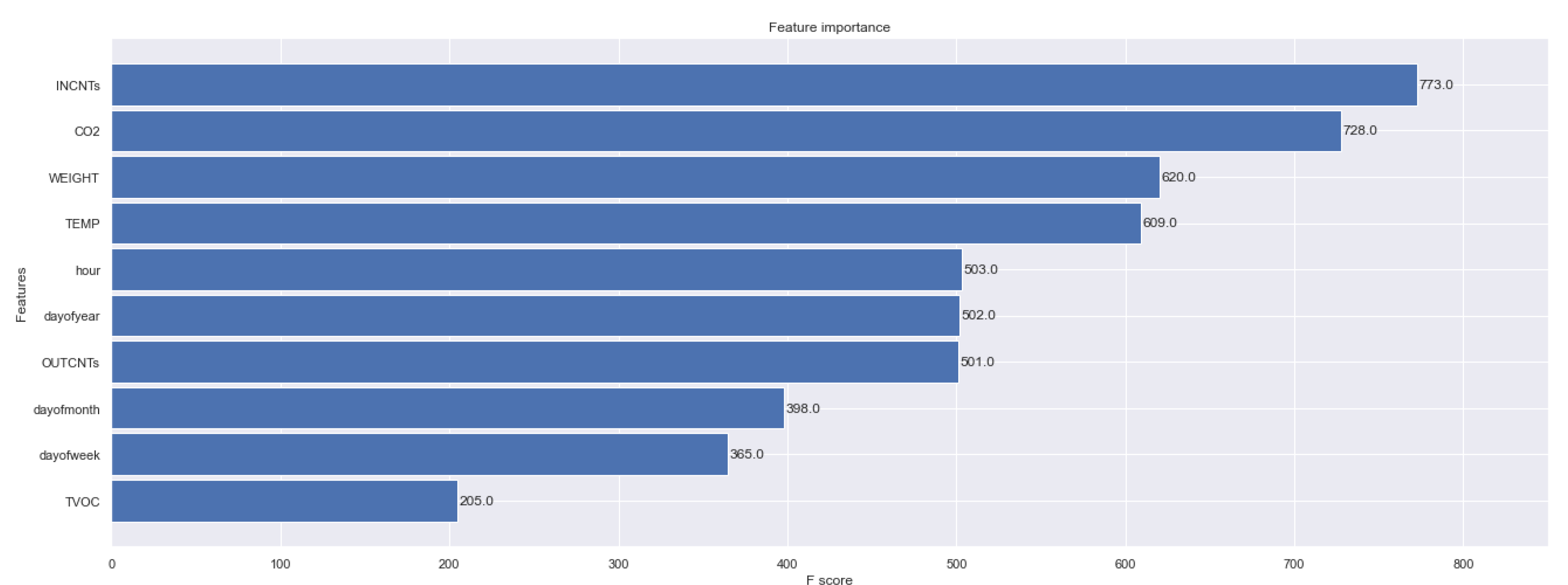
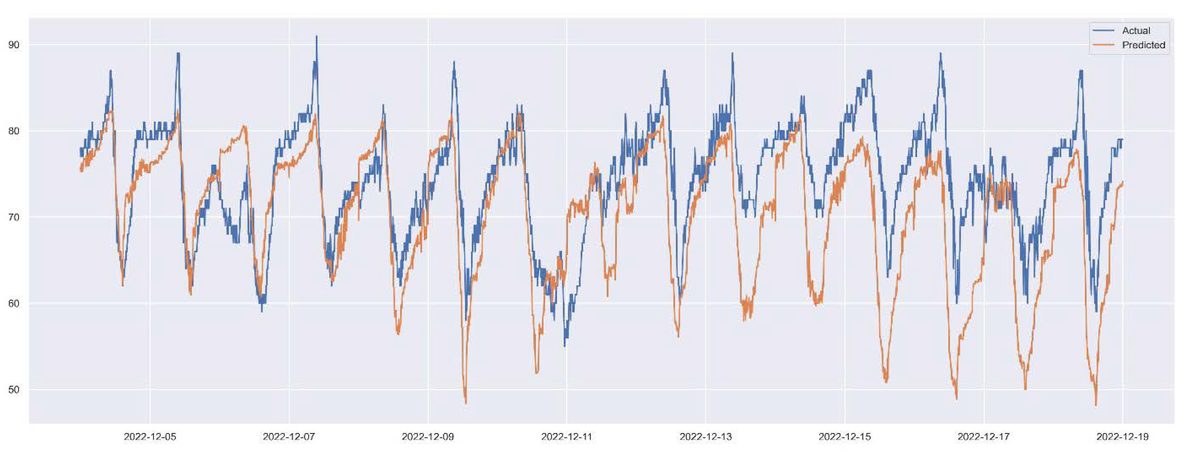
3.8.2. The Xgboost Regression Results
4. Concluding Remarks and Further Steps
Supplementary Materials
Author Contributions
Funding
Institutional Review Board Statement
Informed Consent Statement
Data Availability Statement
Conflicts of Interest
Appendix A
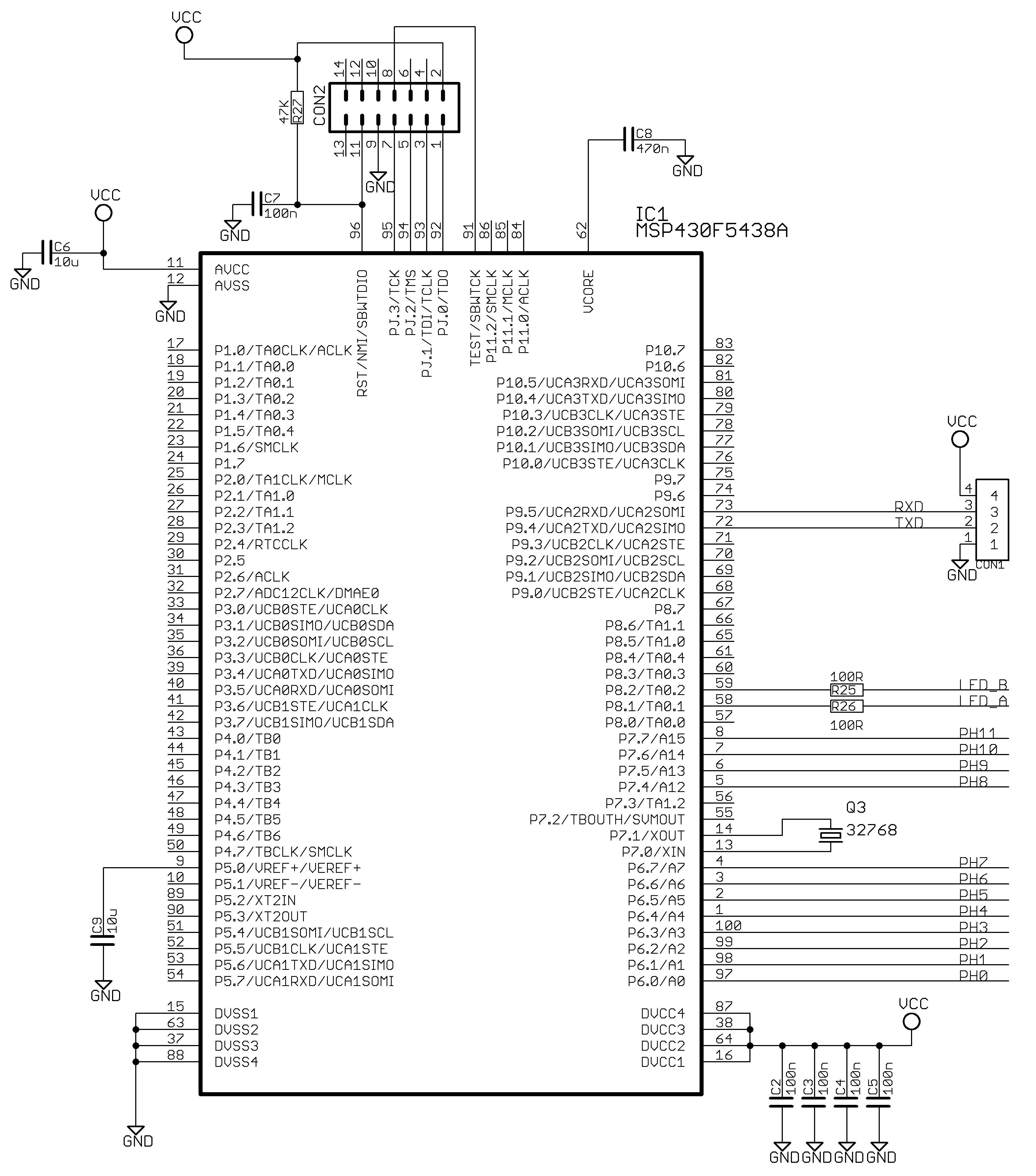
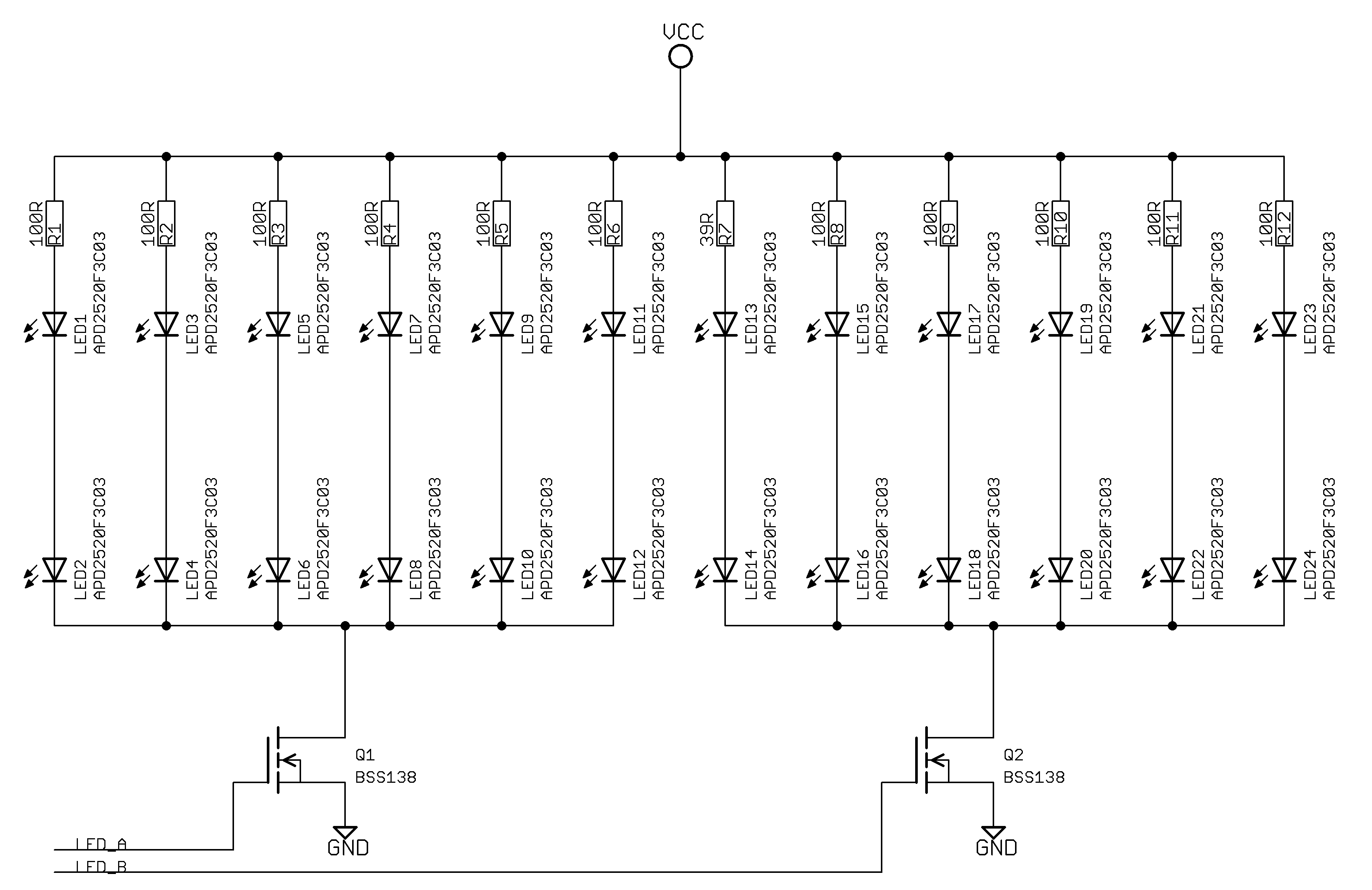
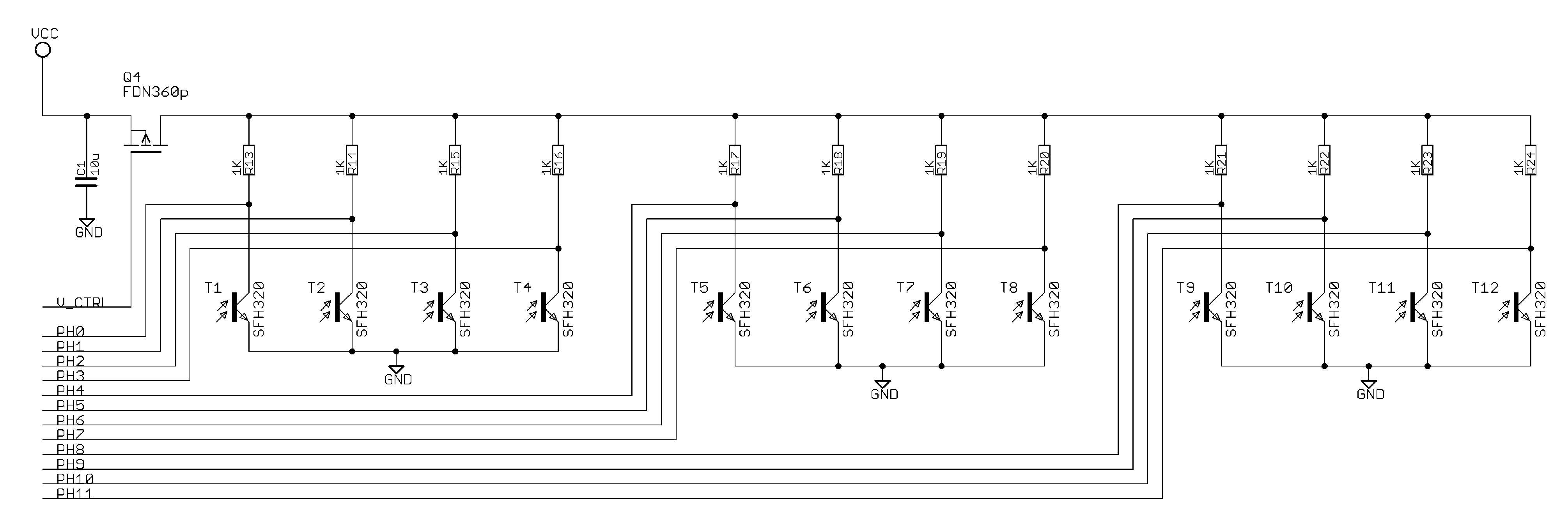
Appendix A.1. Bee Counter


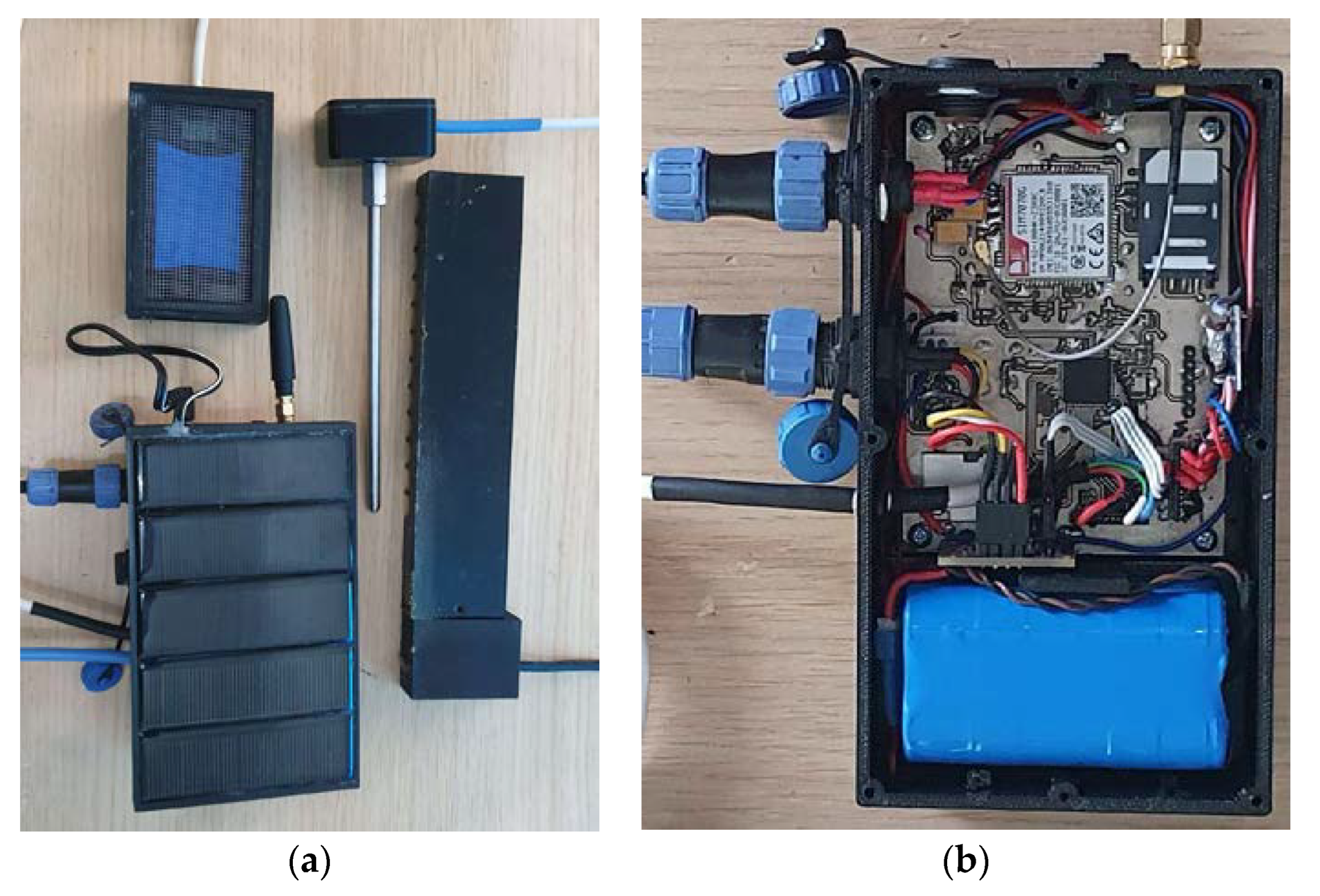
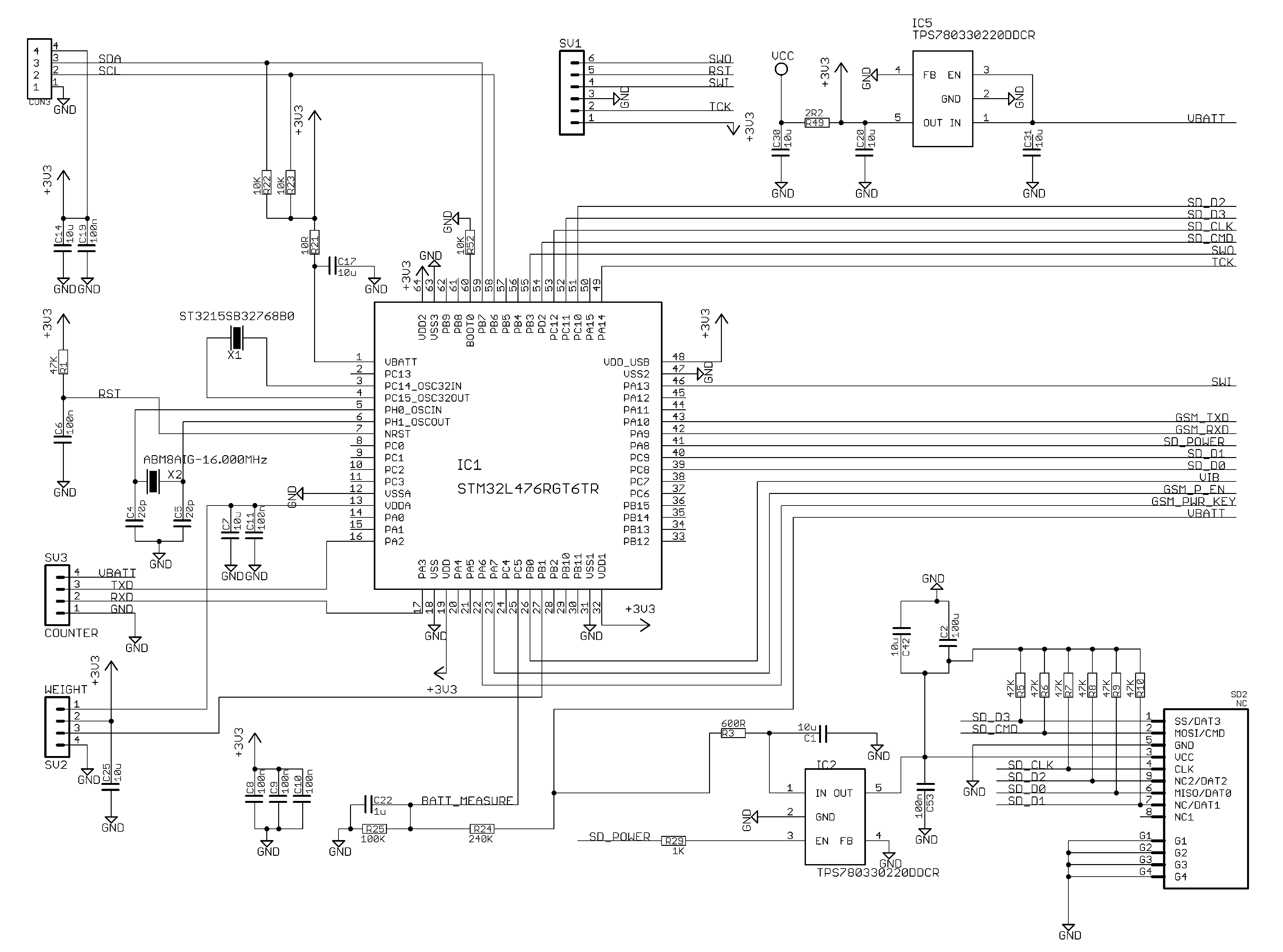
Appendix A.2. Main Board

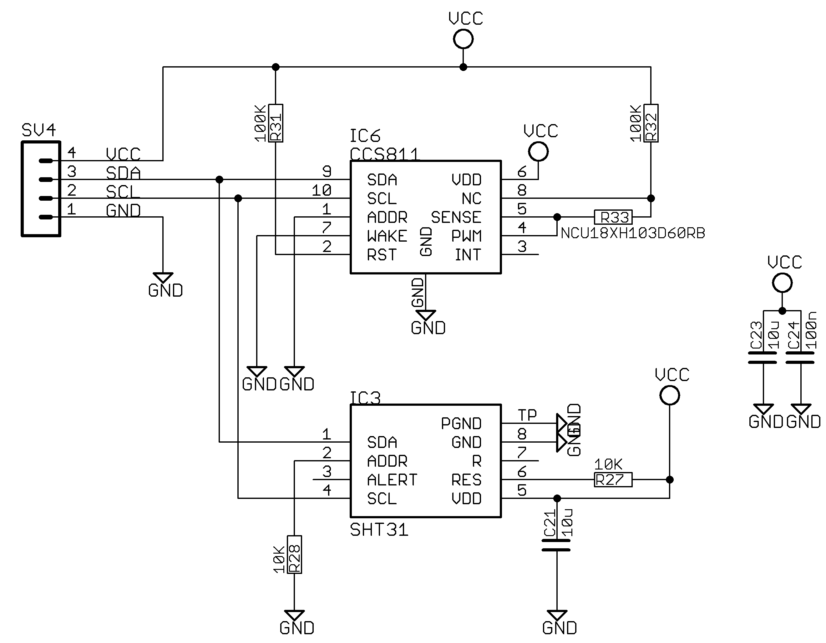
Appendix A.3. Gas Sensors, Temperature and Humidity

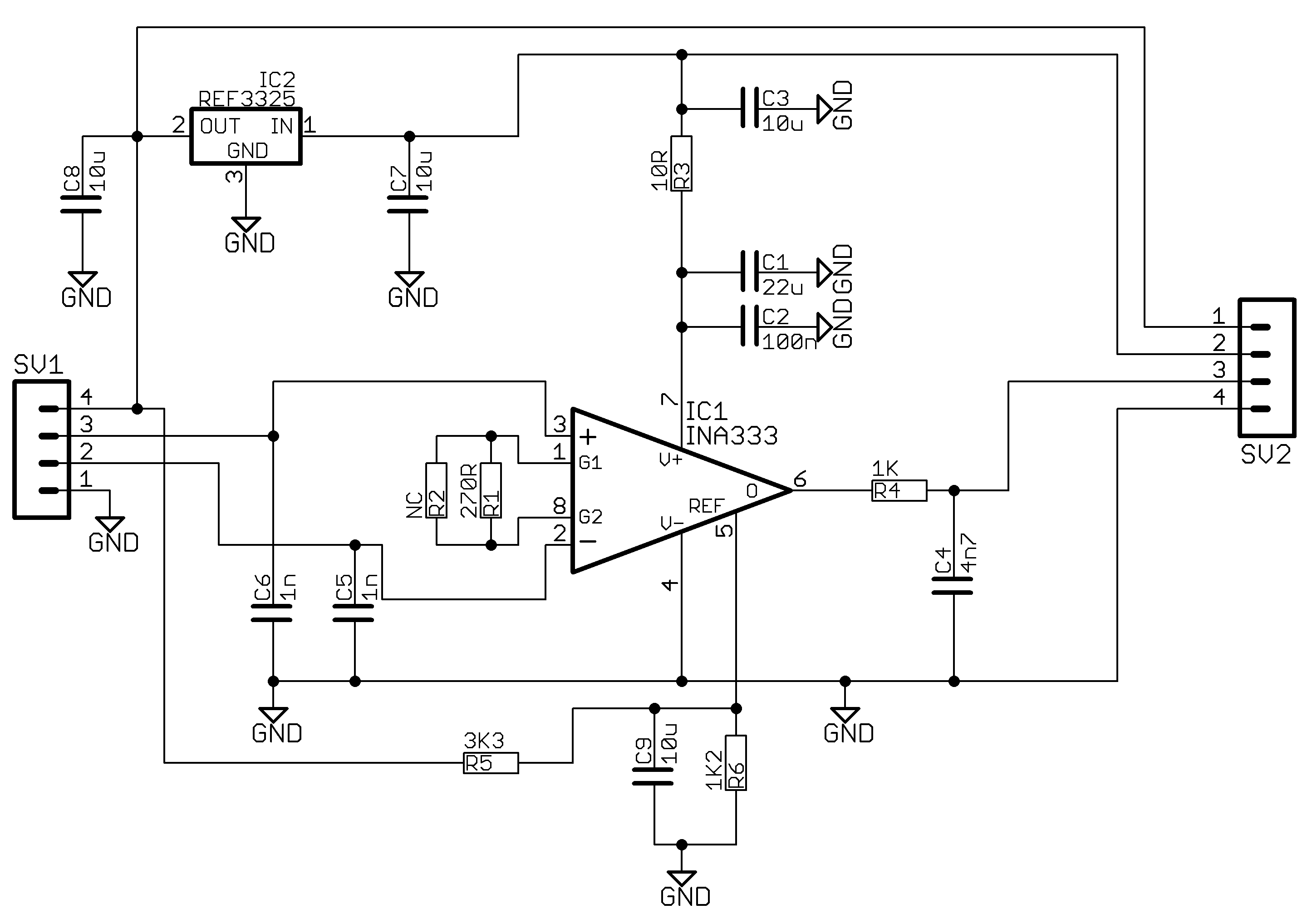
Appendix A.4. Weight Scale

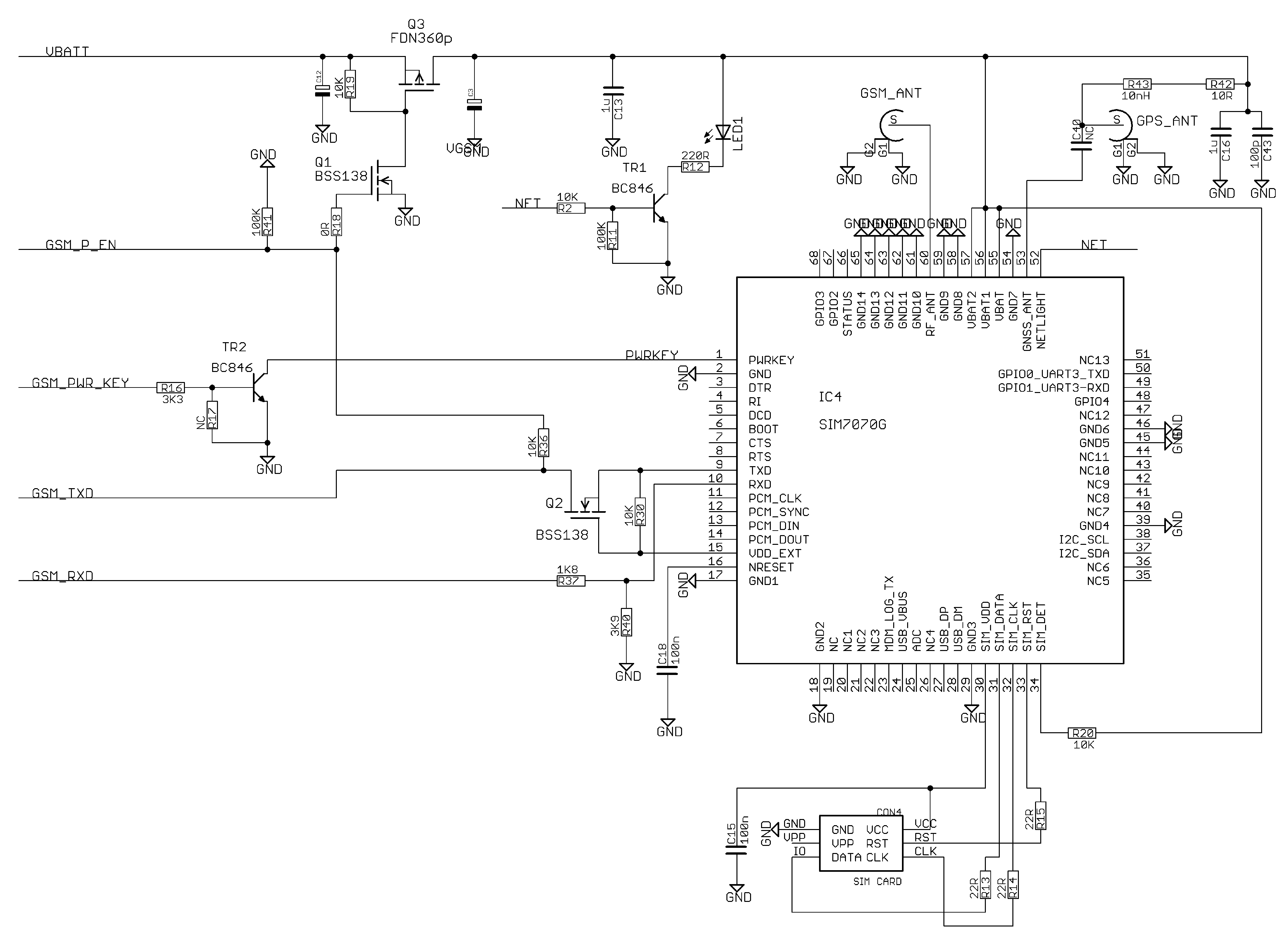
Appendix A.5. Communications

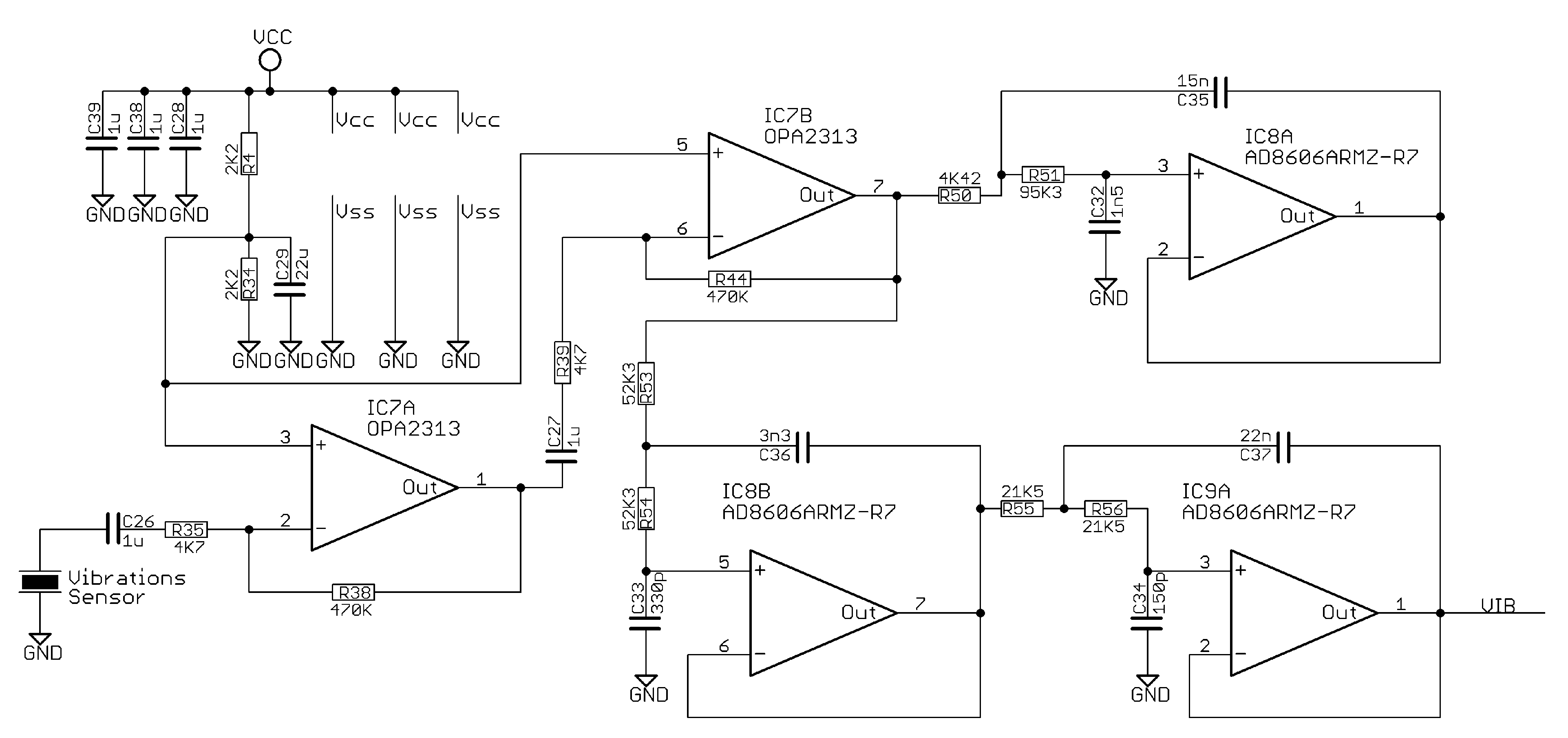
Appendix A.6. Vibrations Sensor

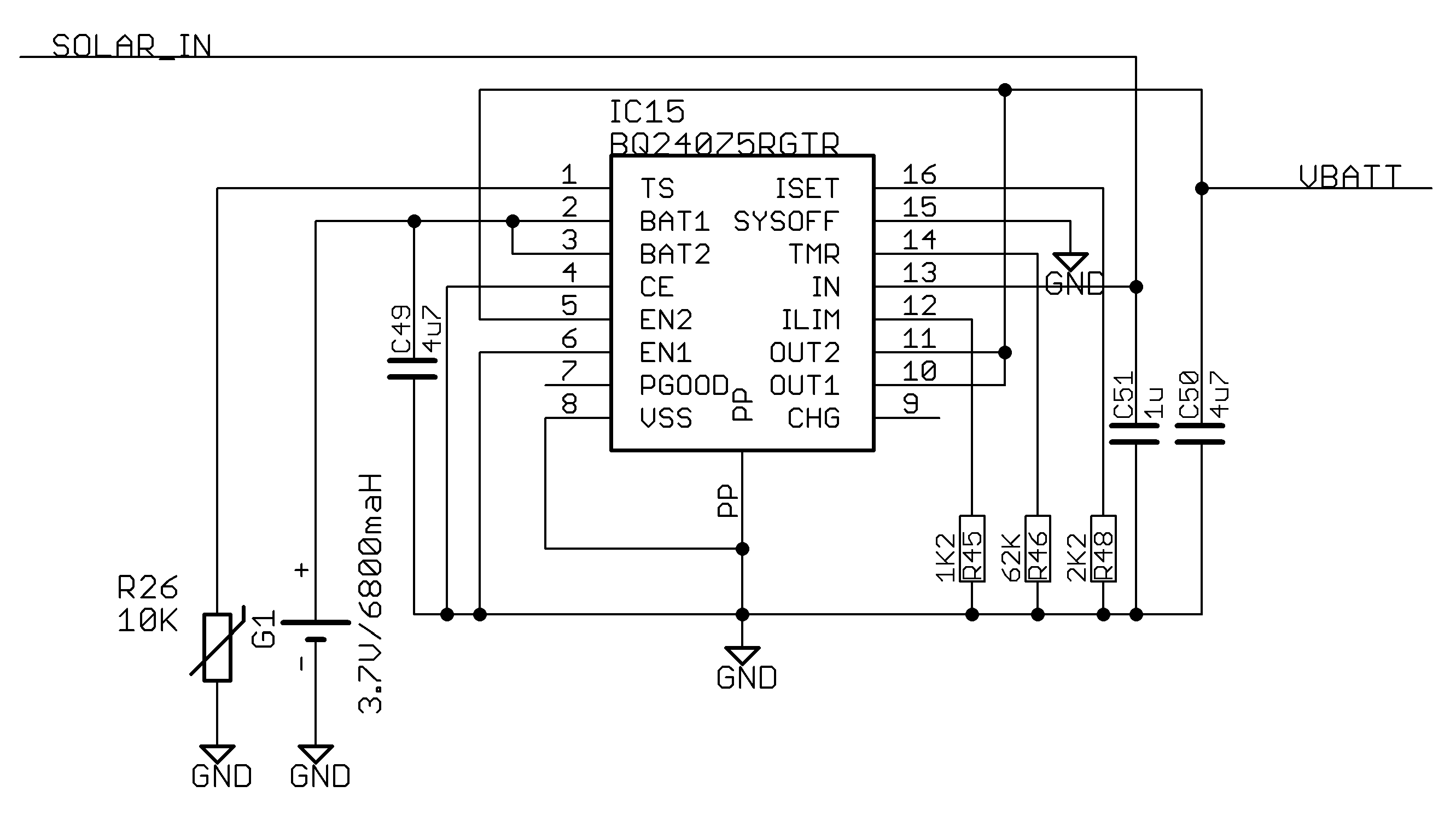
Appendix A.7. Power Regulation

References
- Watson, K.; Stallins, A. Honey Bees and Colony Collapse Disorder: A Pluralistic Reframing. Geogr. Compass 2016, 10, 222–236. [Google Scholar] [CrossRef]
- Available online: https://ec.europa.eu/commission/presscorner/detail/en/IP_19_6777 (accessed on 10 January 2023).
- Gallai, N.; Salles, J.-M.; Settele, J.; Vaissière, B.E. Economic valuation of the vulnerability of world agriculture confronted with pollinator decline. Ecol. Econ. 2009, 68, 810–821. [Google Scholar] [CrossRef]
- Klein, A.-M.; Vaissière, B.E.; Cane, J.H.; Steffan-Dewenter, I.; Cunningham, S.A.; Kremen, C.; Tscharntke, T. Importance of pollinators in changing landscapes for world crops. Proc. R. Soc. B 2006, 274, 303–313. [Google Scholar] [CrossRef]
- Potts, S.G.; Biesmeijer, J.C.; Kremen, C.; Neumann, P.; Schweiger, O.; Kunin, W.E. Global Pollinator Declines: Trends, Impacts and Drivers. Trends Ecol. Evol. 2010, 30, 1–9. [Google Scholar] [CrossRef] [PubMed]
- De la Ruá, P.; Jaffé, R.; Dall, O.; Munoz, I.; Serrano, J. Biodiversity, conservation and current threats to European Honey bees. Apidologie 2009, 40, 263–284. [Google Scholar] [CrossRef]
- Williams, I.H. Aspects of bee diversity and crop pollination in the European Union. In The Conservation of Bees; Metheson, A., Ed.; Academic Press: Cambridge, MA, USA, 1996; pp. 63–80. [Google Scholar]
- Hallmann, C.A.; Sorg, M.; Jongejans, E.; Siepel, H.; Hofland, N.; Schwan, H.; Stenmans, W.; Muller, A.; Sumser, H.; Horren, T.; et al. More than 75 percent decline over 27 years in total flying insect biomass in protected areas. PLoS ONE 2017, 12, e0185809. [Google Scholar] [CrossRef]
- Abdollahi, M.; Giovenazzo, P.; Falk, T.H. Automated Beehive Acoustics Monitoring: A Comprehensive Review of the Literature and Recommendations for Future Work. Appl. Sci. 2022, 12, 3920. [Google Scholar] [CrossRef]
- Hadjur, H.; Ammar, D.; Lefèvre, L. Toward an intelligent and efficient beehive: A survey of precision beekeeping systems and services. Comput. Electron. Agric. 2022, 192, 106604. [Google Scholar] [CrossRef]
- Cecchi, S.; Spinsante, S.; Terenzi, A.; Orcioni, S. A Smart Sensor-Based Measurement System for Advanced Beehive Monitoring. Sensors 2020, 20, 2726. [Google Scholar] [CrossRef]
- Szczurek, A.; Maciejewska, M.; Bak, B.; Wilde, J.; Siuda, M. Semiconductor gas sensor as a detector of Varroa destructor infestation of honey bee colonies—Statistical evaluation. Comput. Electron. Agric. 2019, 162, 405–411. [Google Scholar] [CrossRef]
- Szczurek, A.; Maciejewska, M. Beehive Air Sampling and Sensing Device Operation in Apicultural Applications—Methodological and Technical Aspects. Sensors 2021, 21, 4019. [Google Scholar] [CrossRef] [PubMed]
- Terenzi, A.; Cecchi, S.; Spinsante, S. On the Importance of the Sound Emitted by Honey Bee Hives. Veter. Sci. 2020, 7, 168. [Google Scholar] [CrossRef] [PubMed]
- Ramsey, M.-T.; Bencsik, M.; Newton, M.I.; Reyes, M.; Pioz, M.; Crauser, D.; Delso, N.S.; Le Conte, Y. The prediction of swarming in honeybee colonies using vibrational spectra. Sci. Rep. 2020, 10, 9798. [Google Scholar] [CrossRef]
- Zgank, A. Bee swarm activity acoustic classification for an IoT-based farm service sensors. Sensors 2020, 20, 21. [Google Scholar] [CrossRef] [PubMed]
- Zgank, A. IoT-Based Bee Swarm Activity Acoustic Classification Using Deep Neural Networks. Sensors 2021, 21, 676. [Google Scholar] [CrossRef]
- Ramsey, M.; Bencsik, M.; Newton, M. Long-term trends in the honeybee ‘whooping signal’ revealed by automated detection. PLoS ONE 2017, 12, e0171162. [Google Scholar]
- Marchal, P.; Buatois, A.; Kraus, S.; Klein, S.; Gomez-Moracho, T.; Lihoreau, M. Automated monitoring of bee behaviour using connected hives: Towards a computational apidology. Apidologie 2020, 51, 356–368. [Google Scholar] [CrossRef]
- Gil-Lebrero, S.; Quiles-Latorre, F.J.; Ortiz-López, M.; Sánchez-Ruiz, V.; Gámiz-López, V.; Luna-Rodríguez, J.J. Honey Bee Colonies Remote Monitoring System. Sensors 2017, 17, 55. [Google Scholar] [CrossRef]
- Henry, E.; Adamchuk, V.; Stanhope, T.; Buddle, C.; Rindlaub, N. Precision apiculture: Development of a wireless sensor network for honeybee hives. Comput. Electron. Agric. 2018, 156, 138–144. [Google Scholar] [CrossRef]
- Hong, W.; Xu, B.; Chi, X.; Cui, X.; Yan, Y.; Li, T. Long-Term and Extensive Monitoring for Bee Colonies Based on Internet of Things. IEEE Internet Things J. 2020, 7, 7148–7155. [Google Scholar] [CrossRef]
- Souza Cunha, A.E.; Rose, J.; Prior, J.; Aumann, H.M.; Emanetoglu, N.W.; Drummond, F.A. A novel non-invasive radar to monitor honeybee colony health. Comput. Electron. Agric. 2020, 170, 105241. [Google Scholar] [CrossRef]
- Andrijević, N.; Urošević, V.; Arsić, B.; Herceg, D.; Savić, B. IoT Monitoring and Prediction Modeling of Honeybee Activity with Alarm. Electronics 2022, 11, 783. [Google Scholar] [CrossRef]
- Odemer, R. Approaches, challenges and recent advances in automated bee counting devices: A review. Ann. Appl. Biol. 2021, 180, 73–89. [Google Scholar] [CrossRef]
- Borlinghaus, P.; Odemer, R.; Tausch, F.; Schmidt, K.; Grothe, O. Honeybee counter evaluation—Introducing a novel protocol for measuring daily loss accuracy. Comput. Electron. Agric. 2022, 197, 106957. [Google Scholar] [CrossRef]
- Ntawuzumunsi, E.; Kumaran, S.; Sibomana, L. Self-Powered Smart Beehive Monitoring and Control System (SBMaCS). Sensors 2021, 21, 3522. [Google Scholar] [CrossRef] [PubMed]
- Alsharef, A.; Aggarwal, K.; Sonia; Kumar, M.; Mishra, A. Review of ML and AutoML Solutions to Forecast Time-Series Data. Arch. Comput. Methods Eng. 2022, 29, 5297–5311. [Google Scholar] [CrossRef] [PubMed]
- Hewamalage, H.; Bergmeir, C.; Bandara, K. Recurrent Neural Networks for Time Series Forecasting: Current status and future directions. Int. J. Forecast. 2021, 37, 388–427. [Google Scholar] [CrossRef]
- Ngo, T.-N.; Rustia, D.; Yang, E.-C.; Lin, T.-T. Honeybee Colony Population Daily Loss Rate Forecasting and an Early Warning Method Using Temporal Convolutional Networks. Sensors 2021, 21, 3900. [Google Scholar] [CrossRef]
- Hennessy, G.; Harris, C.; Eaton, C.; Wright, P.; Jackson, E.; Goulson, D.; Ratnieks, F.F. Gone with the wind: Effects of wind on honeybee visit rate and foraging behavior. Anim. Behav. 2020, 161, 23–31. [Google Scholar] [CrossRef]
- Meikle, W.G.; Barg, A.; Weiss, M. Honey bee colonies maintain CO2 and temperature regimes in spite of change in hive ventilation characteristics. Apidologie 2022, 53, 51. [Google Scholar] [CrossRef]
- König, A. An in-hive soft sensor based on phase space features for Varroa infestation level estimation and treatment need detection. J. Sens. Sens. Syst. 2022, 11, 29–40. [Google Scholar] [CrossRef]
- Schlegel, T.; Visscher, P.K.; Seeley, T.D. Beeping and piping: Characterization of two mechano-acoustic signals used by honeybees in swarming. Naturwissenschaften 2012, 99, 1067–1071. [Google Scholar] [CrossRef] [PubMed]
- Schneider, S.S.; Gary, N.E. ‘Quacking’: A Sound Produced by Worker Honeybees after Exposure to Carbon Dioxide. J. Apic. Res. 1984, 23, 25–30. [Google Scholar] [CrossRef]
- Seeley, T.D.; Tautz, J. Worker piping in honeybee swarms and its role in preparing for liftoff. J. Comp. Physiol. A 2001, 187, 667–676. [Google Scholar] [CrossRef]
- Simpson, J.; Cherry, S.M. Queen confinement, queen piping and swarming in Apis mellifera colonies. Anim. Behav. 1969, 17, 271–278. [Google Scholar] [CrossRef]
- Spangler, H.G. Effects of Recorded Queen Pipings and of Continuous Vibration on the Emergence of Queen Honey Bees. Ann. Entomol. Soc. Am. 1971, 64, 50–51. [Google Scholar] [CrossRef]
- Thom, C.; Gilley, D.C. Worker piping in honey bees (Apis mellifera): The behavior of piping nectar foragers. Behav. Ecol. Sociobiol. 2003, 53, 199–205. [Google Scholar] [CrossRef]
- Wenner, A.M. Sound production during the waggle dance of the honeybee. Anim. Behav. 1962, 10, 79–95. [Google Scholar] [CrossRef]
- Woods, E.F. Electronic Prediction of Swarming in Bees. Nature 1959, 184, 842–844. [Google Scholar] [CrossRef]
- Catalano, C.; Paiano, L.; Calabrese, F.; Cataldo, M.; Mancarella, L.; Tommasi, F. Anomaly detection in smart agriculture systems. Comput. Ind. 2022, 143, 103750. [Google Scholar] [CrossRef]
- Kirchner, W.H. Vibrational signals in the tremble dance of the honeybee, Apis mellifera. Behav. Ecol. Sociobiol. 1993, 33, 169–172. [Google Scholar] [CrossRef]
- Tsujiuchi, S.; Sivan-Loukianova, E.; Eberl, D.F.; Kitagawa, Y.; Kadowaki, T. Dynamic Range Compression in the Honey Bee Auditory System toward Waggle Dance Sounds. PLoS ONE 2007, 2, e234. [Google Scholar] [CrossRef] [PubMed]
- Pratt, S.; Kühnholz, S.; Seeley, T.D.; Weidenmüller, A. Worker piping associated with foraging in undisturbed queenright colonies of honey bees. Apidologie 1996, 27, 13–20. [Google Scholar] [CrossRef]
- Hrncir, M.; Maia-Silva, C.; Farina, W.M. Honey bee workers generate low-frequency vibrations that are reliable indicators of their activity level. J. Comp. Physiol. A Neuroethol. Sens Neural. Behav. Physiol. 2019, 205, 79–86. [Google Scholar] [CrossRef] [PubMed]
- Kraus, H.; Velthius, H.H.W. High Humidity in the Honey Bee (Apis mellifera L.) Brood Nest Limits Reproduction of the Parasitic Mite Varroa jacobsoni Oud. Naturwissenschaften 1997, 84, 217–218. [Google Scholar] [CrossRef]
- Guidance on the risk assessment of plant protection products on bees (Apis mellifera, Bombus spp. and solitary bees). EFSA J. 2013, 11, 3295. [CrossRef]
- Ippolito, A.; del Aguila, M.; Aiassa, E.; Guajardo, I.M.; Neri, F.M.; Alvarez, F.; Mosbach-Schulz, O.; Szentes, C. Review of the evidence on bee background mortality. EFSA Support. Publ. 2020, 17, 1880E. [Google Scholar] [CrossRef]
- Januschowski, T.; Wang, Y.; Torkkola, K.; Erkkilä, T.; Hasson, H.; Gasthaus, J. Forecasting with trees. Int. J. Forecast. 2022, 38, 1473–1481. [Google Scholar] [CrossRef]
- Tashakkori, R.; Hamza, A.S.; Crawford, M.B. Beemon: An IoT-based beehive monitoring system. Comput. Electron. Agric. 2021, 190, 106427. [Google Scholar] [CrossRef]
- Edwards-Murphy, F.; Magno, M.; Whelan, P.M.; O’Halloran, J.; Popovici, E.M. b+WSN: Smart beehive with preliminary decision tree analysis for agriculture and honeybee health monitoring. Comput. Electron. Agric. 2016, 124, 211–219. [Google Scholar] [CrossRef]


| Audio Signal | Freq. Bands (Hz) | Role | References |
|---|---|---|---|
| Whooping | 300–450 | begging call or stop signal | [18] |
| Queen piping | 400–500 | swarming, young queens to signal readiness for battle with the mature queen | [37] |
| Queen quacking | 200–350 | quacking follows tooting, confined queens responses | [40] |
| Tremble | 300–450 | foragers returning to the hive, stimulates additional bees to function as nectar receivers | [42] |
| Waggle | 250–300 | recruitment to feeding sites, inform nestmates about direction and distance to locations of attractive food | [43] |
| Tooting | 200-350, 400-500 | young queens to signal readiness for battle with the mature queen | [44] |
| Worker piping | 100–250, 330–430 | liftoff | [36,45] |
| Low signals | 0–100 | indicators of worker bees activity level | [46] |
| TRAIN | TEST | |
|---|---|---|
| MAPE | 5.99 | 5.01 |
| R2 | 72.84 | 45.62 |
| TRAIN | TEST | |
|---|---|---|
| MAPE | 1.67 | 8.36 |
| R2 | 97.59 | −17.49 |
Disclaimer/Publisher’s Note: The statements, opinions and data contained in all publications are solely those of the individual author(s) and contributor(s) and not of MDPI and/or the editor(s). MDPI and/or the editor(s) disclaim responsibility for any injury to people or property resulting from any ideas, methods, instructions or products referred to in the content. |
© 2023 by the authors. Licensee MDPI, Basel, Switzerland. This article is an open access article distributed under the terms and conditions of the Creative Commons Attribution (CC BY) license (https://creativecommons.org/licenses/by/4.0/).
Share and Cite
Rigakis, I.; Potamitis, I.; Tatlas, N.-A.; Psirofonia, G.; Tzagaraki, E.; Alissandrakis, E. A Low-Cost, Low-Power, Multisensory Device and Multivariable Time Series Prediction for Beehive Health Monitoring. Sensors 2023, 23, 1407. https://doi.org/10.3390/s23031407
Rigakis I, Potamitis I, Tatlas N-A, Psirofonia G, Tzagaraki E, Alissandrakis E. A Low-Cost, Low-Power, Multisensory Device and Multivariable Time Series Prediction for Beehive Health Monitoring. Sensors. 2023; 23(3):1407. https://doi.org/10.3390/s23031407
Chicago/Turabian StyleRigakis, Iraklis, Ilyas Potamitis, Nicolas-Alexander Tatlas, Giota Psirofonia, Efsevia Tzagaraki, and Eleftherios Alissandrakis. 2023. "A Low-Cost, Low-Power, Multisensory Device and Multivariable Time Series Prediction for Beehive Health Monitoring" Sensors 23, no. 3: 1407. https://doi.org/10.3390/s23031407
APA StyleRigakis, I., Potamitis, I., Tatlas, N.-A., Psirofonia, G., Tzagaraki, E., & Alissandrakis, E. (2023). A Low-Cost, Low-Power, Multisensory Device and Multivariable Time Series Prediction for Beehive Health Monitoring. Sensors, 23(3), 1407. https://doi.org/10.3390/s23031407