
A Density-Based Multilevel Terrain-Adaptive Noise Removal Method for ICESat-2 Photon-Counting Data


Abstract
:1. Introduction
2. Materials
2.1. ICESat2 Data
2.2. Validation Data
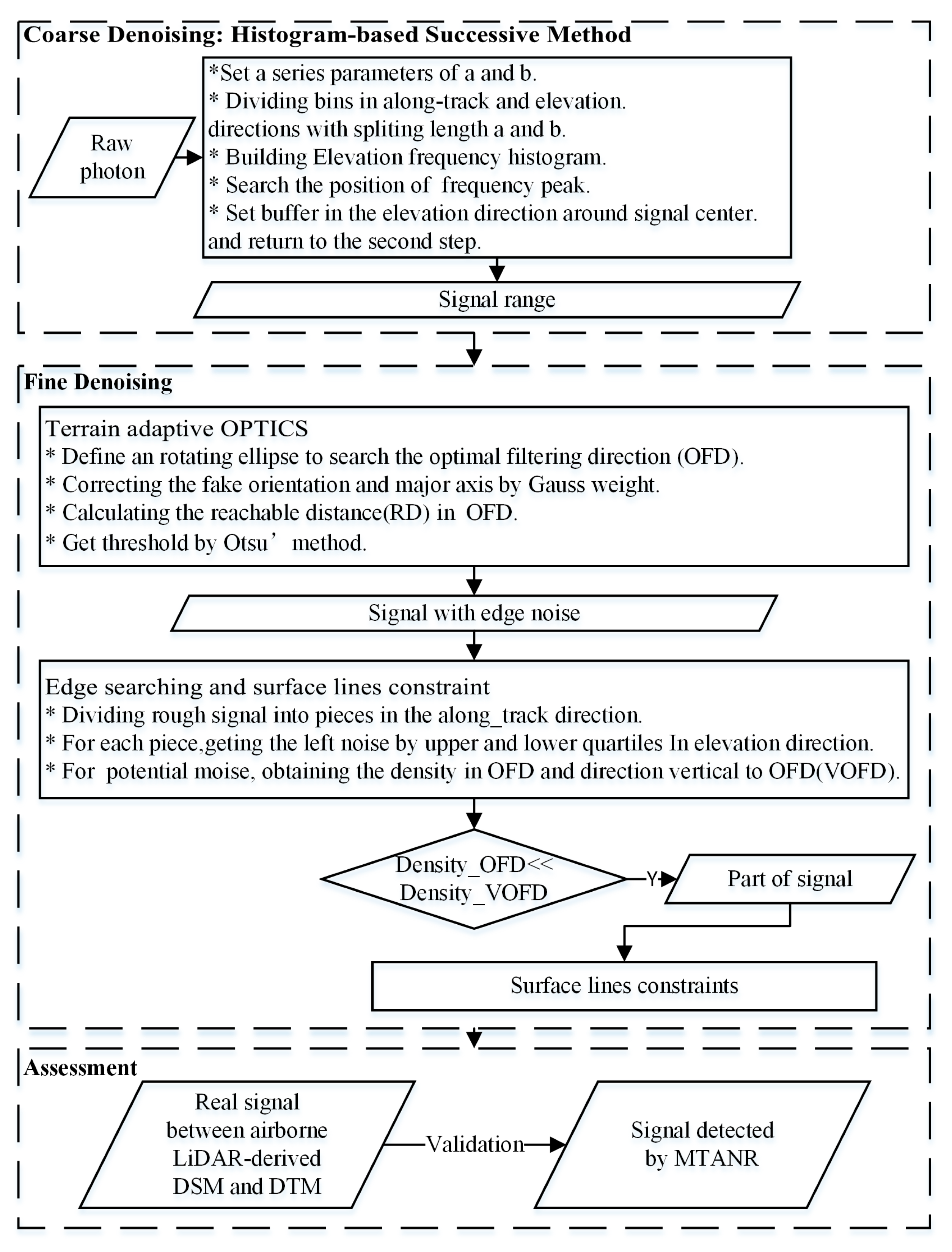
3. Method
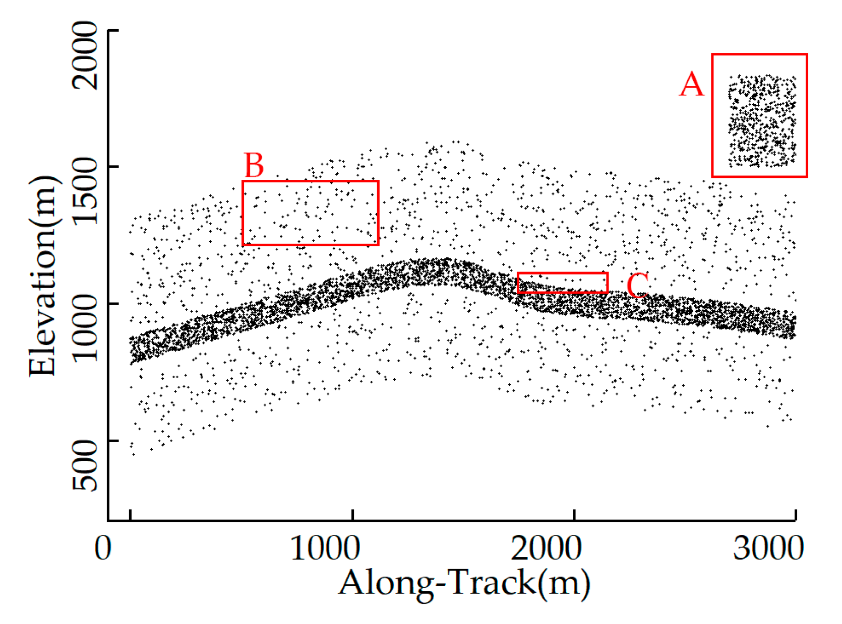
3.1. Preprocessing
3.2. Terrain-Adaptive OPTICS Algorithm
3.2.1. Definition of Rotating Ellipsoidal OPTICS
3.2.2. Optimal Filtering Direction Searching and Parameter Correction
3.3. Edge Searching and Surface Lines Constraints
3.4. Accuracy Assessment
4. Experiment Results and Analysis
4.1. Coarse Denoising: Histogram-Based Successive Denoising
4.2. Fine Denoising: Terrain-Adaptive OPTICS and Edge Searching
4.3. Comparative Analysis of Several Methods in Typical Areas
4.4. Algorithm Robustness Analysis
4.5. Challenge under Extremely Dense Vegetation
5. Conclusions
- (1)
- The rotatably elliptical search domain can adapt to complex terrains and effectively utilize slope information. Compared to typical algorithms with fixed search domains, the proposed MTANR robustly retains sparse signals in steep areas and terrains with abrupt changes.
- (2)
- Edge searching improves the ability to distinguish between signal and edge noise, which effectively improves denoising performance and minimizes the effects of edge noise in ICESat2 data applications like canopy height inversion.
Author Contributions
Funding
Institutional Review Board Statement
Informed Consent Statement
Data Availability Statement
Acknowledgments
Conflicts of Interest
Appendix A

| Datasets | Parameters | Descriptions [17,18] |
|---|---|---|
| ATL03 | signal_conf_ph | Confidence level associated with each photon event selected as the signal. (0 = noise, 1 = added to allow for buffering but the algorithm classifies it as background, 2 = low, 3 = med, and 4 = high.) |
| segment_id | A 7-digit number identifies the along-track geolocation segment number. | |
| ATL08 | classed_pc_flag | Land Vegetation ATBD classification flag for each photon as either noise, ground, canopy, or top of canopy. (0 = noise, 1 = ground, 2 = canopy, and 3 = top of canopy.) |
| classed_pc_indx | Index (1-based) of the ATL08 classified signal photon from the start of the ATL03 geolocation segment specified on the ATL08 product at the photon rate in the corresponding parameter, ph_segment_id. This index traces back to the specific photon within a 20 m segment_id on ATL03. | |
| ph_segment_id | Segment ID of photons tracing back to specific 20 m segment_id on ATL03. |
References
- Lin, X.; Shang, R.; Chen, J.M.; Zhao, G.; Zhang, X.; Huang, Y.; Yu, G.; He, N.; Xu, L.; Jiao, W. High-resolution forest age mapping based on forest height maps derived from GEDI and ICESat-2 space-borne lidar data. Agric. For. Meteorol. 2023, 339, 109592. [Google Scholar] [CrossRef]
- Akturk, E.; Popescu, S.C.C.; Malambo, L. ICESat-2 for Canopy Cover Estimation at Large-Scale on a Cloud-Based Platform. Sensors 2023, 23, 3394. [Google Scholar] [CrossRef] [PubMed]
- Gao, S.; Zhu, J.; Fu, H. A Rapid and Easy Way for National Forest Heights Retrieval in China Using ICESat-2/ATL08 in 2019. Forests 2023, 14, 1270. [Google Scholar] [CrossRef]
- Swatantran, A.; Tang, H.; Barrett, T.; DeCola, P.; Dubayah, R. Rapid, High-Resolution Forest Structure and Terrain Mapping over Large Areas using Single Photon Lidar. Sci. Rep. 2016, 6, 28277. [Google Scholar] [CrossRef] [PubMed]
- Liu, Z.; Zhu, J.; Fu, H.; Zhou, C.; Zuo, T. Evaluation of the Vertical Accuracy of Open Global DEMs over Steep Terrain Regions Using ICESat Data: A Case Study over Hunan Province, China. Sensors 2020, 20, 4865. [Google Scholar] [CrossRef] [PubMed]
- Wang, B.; Ma, Y.; Zhang, J.; Zhang, H.; Zhu, H.; Leng, Z.; Zhang, X.; Cui, A. A noise removal algorithm based on adaptive elevation difference thresholding for ICESat-2 photon-counting data. Int. J. Appl. Earth Obs. Geoinf. 2023, 117, 103207. [Google Scholar] [CrossRef]
- Zhang, G.; Ganguly, S.; Nemani, R.R.; White, M.A.; Milesi, C.; Hashimoto, H.; Wang, W.L.; Saatchi, S.; Yu, Y.F.; Myneni, R.B. Estimation of forest aboveground biomass in California using canopy height and leaf area index estimated from satellite data. Remote Sens. Environ. 2014, 151, 44–56. [Google Scholar] [CrossRef]
- Neuenschwander, A.L.; Magruder, L.A. Canopy and Terrain Height Retrievals with ICESat-2: A First Look. Remote Sens. 2019, 11, 1721. [Google Scholar] [CrossRef]
- An, Z.; Chen, P.; Tang, F.; Yang, X.; Wang, R.; Wang, Z. Evaluating the Performance of Seven Ongoing Satellite Altimetry Missions for Measuring Inland Water Levels of the Great Lakes. Sensors 2022, 22, 9718. [Google Scholar] [CrossRef]
- Jang, J.-Y.; Cho, M. Lensless Three-Dimensional Imaging under Photon-Starved Conditions. Sensors 2023, 23, 2336. [Google Scholar] [CrossRef]
- Neuenschwander, A.; Magruder, L.; Guenther, E.; Hancock, S.; Purslow, M. Radiometric Assessment of ICESat-2 over Vegetated Surfaces. Remote Sens. 2022, 14, 787. [Google Scholar] [CrossRef]
- Jasinski, M.F.; Stoll, J.D.; Cook, W.B.; Ondrusek, M.; Stengel, E.; Brunt, K. Inland and Near-Shore Water Profiles Derived from the High-Altitude Multiple Altimeter Beam Experimental Lidar (MABEL). J. Coast. Res. 2016, 76, 44–55. [Google Scholar] [CrossRef]
- Brunt, K.M.; Neumann, T.A.; Walsh, K.M.; Markus, T. Determination of Local Slope on the Greenland Ice Sheet Using a Multibeam Photon-Counting Lidar in Preparation for the ICESat-2 Mission. IEEE Geosci. Remote Sens. Lett. 2014, 11, 935–939. [Google Scholar] [CrossRef]
- Zhu, X.X.; Nie, S.; Wang, C.; Xi, X.H.; Hu, Z.Y. A Ground Elevation and Vegetation Height Retrieval Algorithm Using Micro-Pulse Photon-Counting Lidar Data. Remote Sens. 2018, 10, 1962. [Google Scholar] [CrossRef]
- Xie, H.; Xu, Q.; Ye, D.; Jia, J.; Sun, Y.; Huang, P.; Li, M.; Liu, S.; Xie, F.; Hao, X.; et al. A Comparison and Review of Surface Detection Methods Using MBL, MABEL, and ICESat-2 Photon-Counting Laser Altimetry Data. IEEE J. Sel. Top. Appl. Earth Obs. Remote Sens. 2021, 14, 7604–7623. [Google Scholar] [CrossRef]
- Neuenschwander, A.; Pitts, K. The ATL08 land and vegetation product for the ICESat-2 Mission. Remote Sens. Environ. 2019, 221, 247–259. [Google Scholar] [CrossRef]
- Neuenschwander, A.; Pitts, K.; Jelley, B.; Robbins, J.; Markel, J.; Popescu, S.; Nelson, R.; Harding, D.; Pederson, D.; Klotz, B.; et al. Ice, Cloud, and Land Elevation Satellite-2 (ICESat-2). Algorithm Theoretical Basis Document (ATBD) for Land—Vegetation Along-Track Products ATL08, (Version 4); NASA National Snow and Ice Data Center Distributed Active Archive Center: Boulder, CO, USA, 2021. [Google Scholar]
- Neuenschwander, A.; Pitts, K.; Jelley, B.; Robbins, J.; Markel, J.; Popescu, S.; Nelson, R.; Harding, D.; Pederson, D.; Klotz, B.; et al. ATLAS/ICESat-2 L3A Land and Vegetation Height, Version 5; NASA National Snow and Ice Data Center Distributed Active Archive Center: Boulder, CO, USA, 2021. [Google Scholar]
- Xia, S.; Wang, C.; Xi, X.; Luo, S.; Zeng, H. Point cloud filtering and tree height estimation using airborne experiment data of ICESat-2. Yaogan Xuebao/J. Remote Sens. 2014, 18, 1199–1207. [Google Scholar] [CrossRef]
- Wang, C.; Ji, M.; Wang, J.; Wen, W.; Li, T.; Sun, Y. An Improved DBSCAN Method for LiDAR Data Segmentation with Automatic Eps Estimation. Sensors 2019, 19, 172. [Google Scholar] [CrossRef]
- Wang, X.; Pan, Z.; Glennie, C. A Novel Noise Filtering Model for Photon-Counting Laser Altimeter Data. IEEE Geosci. Remote Sens. Lett. 2016, 13, 947–951. [Google Scholar] [CrossRef]
- Ester, M.; Kriegel, H.-P.; Sander, J.; Xu, X. A density-based algorithm for discovering clusters in large spatial databases with noise. In Proceedings of the Second International Conference on Knowledge Discovery and Data Mining (KDD’96), Oregon, Portland, 2–4 August 1996; pp. 226–231. [Google Scholar]
- Ankerst, M.; Breunig, M.M.; Kriegel, H.-P.; Sander, J.J.A.S.r. OPTICS: Ordering points to identify the clustering structure. In Proceedings of the ACM SIGMOD International Conference on Management of Data (SIGMOD 1999), Philadelphia, PA, USA, 1–3 June 1999; Volume 28, pp. 49–60. [Google Scholar]
- Zhu, X.; Nie, S.; Wang, C.; Xi, X.; Wang, J.; Li, D.; Zhou, H. A Noise Removal Algorithm Based on OPTICS for Photon-Counting LiDAR Data. IEEE Geosci. Remote Sens. Lett. 2021, 18, 1471–1475. [Google Scholar] [CrossRef]
- Gao, S.; Li, Y.; Zhu, J.; Fu, H.; Zhou, C. Retrieving Forest Canopy Height From ICESat-2 Data by an Improved DRAGANN Filtering Method and Canopy Top Photons Classification. IEEE Geosci. Remote Sens. Lett. 2022, 19, 2505505. [Google Scholar] [CrossRef]
- Huang, J.; Xing, Y.; You, H.; Qin, L.; Tian, J.; Ma, J. Particle Swarm Optimization-Based Noise Filtering Algorithm for Photon Cloud Data in Forest Area. Remote Sens. 2019, 11, 980. [Google Scholar] [CrossRef]
- Zhang, G.; Lian, W.; Li, S.; Cui, H.; Jing, M.; Chen, Z. A Self-Adaptive Denoising Algorithm Based on Genetic Algorithm for Photon-Counting Lidar Data. IEEE Geosci. Remote Sens. Lett. 2022, 19, 6501405. [Google Scholar] [CrossRef]
- Li, Y.; Fu, H.; Zhu, J.; Wang, C. A Filtering Method for ICESat-2 Photon Point Cloud Data Based on Relative Neighboring Relationship and Local Weighted Distance Statistics. IEEE Geosci. Remote Sens. Lett. 2021, 18, 1891–1895. [Google Scholar] [CrossRef]
- He, L.; Pang, Y.; Zhang, Z.; Liang, X.; Chen, B. ICESat-2 data classification and estimation of terrain height and canopy height. Int. J. Appl. Earth Obs. Geoinf. 2023, 118, 103233. [Google Scholar] [CrossRef]
- Li, Y.; Zhu, J.; Fu, H.; Gao, S.; Wang, C. Filtering Photon Cloud Data in Forested Areas Based on Elliptical Distance Parameters and Machine Learning Approach. Forests 2022, 13, 663. [Google Scholar] [CrossRef]
- Chen, B.; Pang, Y.; Li, Z.; Lu, H.; Liang, X. Photon counting LiDAR point cloud data filtering based on random forest algorithm. J. Geo-Inf. Sci. 2019, 21, 898–906. [Google Scholar] [CrossRef]
- Kui, M.; Xu, Y.; Wang, J.; Cheng, F. Research on the Adaptability of Typical Denoising Algorithms Based on ICESat-2 Data. Remote Sens. 2023, 15, 3884. [Google Scholar] [CrossRef]
- Zhang, J.; Kerekes, J. An Adaptive Density-Based Model for Extracting Surface Returns From Photon-Counting Laser Altimeter Data. IEEE Geosci. Remote Sens. Lett. 2015, 12, 726–730. [Google Scholar] [CrossRef]
- Huang, X.; Cheng, F.; Wang, J.; Duan, P.; Wang, J. Forest Canopy Height Extraction Method Based on ICESat-2/ATLAS Data. IEEE Trans. Geosci. Remote Sens. 2023, 61, 5700814. [Google Scholar] [CrossRef]
- Wu, Y.; Zhao, R.; Hu, Q.; Zhang, Y.; Zhang, K. Retrieving Sub-Canopy Terrain from ICESat-2 Data Based on the RNR-DCM Filtering and Erroneous Ground Photons Correction Approach. Remote Sens. 2023, 15, 3904. [Google Scholar] [CrossRef]
- You, H.; Li, Y.; Qin, Z.; Lei, P.; Chen, J.; Shi, X. Research on Multilevel Filtering Algorithm Used for Denoising Strong and Weak Beams of Daytime Photon Cloud Data with High Background Noise. Remote Sens. 2023, 15, 4260. [Google Scholar] [CrossRef]
- Liu, A.; Cheng, X.; Chen, Z. Performance evaluation of GEDI and ICESat-2 laser altimeter data for terrain and canopy height retrievals. Remote Sens. Environ. 2021, 264, 112571. [Google Scholar] [CrossRef]
- Gibbons, A.; Neumann, T.; Hancock, D.; Harbeck, K.; Lee, J. On-Orbit Radiometric Performance on ICESat-2. Earth Space Sci. 2021, 8, e2020EA001503. [Google Scholar] [CrossRef]
- Huang, J.; Xing, Y.; Shuai, Y.; Zhu, H. A Novel Noise Filtering Evaluation Criterion of ICESat-2 Signal Photon Data in Forest Environments. IEEE Geosci. Remote Sens. Lett. 2022, 19, 7003805. [Google Scholar] [CrossRef]
- Nan, Y.; Feng, Z.; Li, B.; Liu, E. Multiscale Fusion Signal Extraction for Spaceborne Photon-Counting Laser Altimeter in Complex and Low Signal-to-Noise Ratio Scenarios. IEEE Geosci. Remote Sens. Lett. 2022, 19, 1000105. [Google Scholar] [CrossRef]
- Rodda, S.R.; Nidamanuri, R.R.; Fararoda, R.; Mayamanikandan, T.; Rajashekar, G. Evaluation of Height Metrics and Above-Ground Biomass Density from GEDI and ICESat-2 Over Indian Tropical Dry Forests using Airborne LiDAR Data. J. Indian Soc. Remote Sens. 2023. [Google Scholar] [CrossRef]
- Zhang, T.; Liu, D. Improving ICESat-2-based boreal forest height estimation by a multivariate sample quality control approach. Methods Ecol. Evol. 2023, 14, 1623–1638. [Google Scholar] [CrossRef]
- Adam, M.; Urbazaev, M.; Dubois, C.; Schmullius, C. Accuracy Assessment of GEDI Terrain Elevation and Canopy Height Estimates in European Temperate Forests: Influence of Environmental and Acquisition Parameters. Remote Sens. 2020, 12, 3948. [Google Scholar] [CrossRef]
- Lahssini, K.; Baghdadi, N.; le Maire, G.; Fayad, I. Influence of GEDI Acquisition and Processing Parameters on Canopy Height Estimates over Tropical Forests. Remote Sens. 2022, 14, 6264. [Google Scholar] [CrossRef]
- Sothe, C.; Gonsamo, A.; Lourenco, R.B.; Kurz, W.A.; Snider, J. Spatially Continuous Mapping of Forest Canopy Height in Canada by Combining GEDI and ICESat-2 with PALSAR and Sentinel. Remote Sens. 2022, 14, 5158. [Google Scholar] [CrossRef]
- Nie, S.; Wang, C.; Xi, X.; Luo, S.; Li, G.; Tian, J.; Wang, H. Estimating the vegetation canopy height using micro-pulse photon-counting LiDAR data. Opt. Express 2018, 26, A520–A540. [Google Scholar] [CrossRef] [PubMed]
- Xie, H.; Ye, D.; Xu, Q.; Sun, Y.; Huang, P.; Tong, X.; Guo, Y.; Liu, X.; Liu, S. A Density-Based Adaptive Ground and Canopy Detecting Method for ICESat-2 Photon-Counting Data. IEEE Trans. Geosci. Remote Sens. 2022, 60, 4411813. [Google Scholar] [CrossRef]
- Barros, W.K.P.; Dias, L.A.; Fernandes, M.A.C. Fully Parallel Implementation of Otsu Automatic Image Thresholding Algorithm on FPGA. Sensors 2021, 21, 4151. [Google Scholar] [CrossRef] [PubMed]
- Yang, P.; Fu, H.; Zhu, J.; Li, Y.; Wang, C. An Elliptical Distance Based Photon Point Cloud Filtering Method in Forest Area. IEEE Geosci. Remote Sens. Lett. 2022, 19, 6504705. [Google Scholar] [CrossRef]
- Chen, X.; Li, J.; Huang, S.; Cui, H.; Liu, P.; Sun, Q. An Automatic Concrete Crack-Detection Method Fusing Point Clouds and Images Based on Improved Otsu’s Algorithm. Sensors 2021, 21, 1581. [Google Scholar] [CrossRef] [PubMed]
- Li, Y.; Fu, H.; Zhu, J.; Wang, L.; Zhao, R.; Wang, C. A Photon Cloud Filtering Method in Forested Areas Considering the Density Difference Between Canopy Photons and Ground Photons. IEEE Trans. Geosci. Remote Sens. 2023, 61, 4403114. [Google Scholar] [CrossRef]
- Shuaitai, Z.; Guoyuan, L.; Xiaoqing, Z.; Jiaqi, Y.; Jinquan, G.; Xinming, T. Single photon point cloud denoising algorithm based on multi-features adaptive. Infrared Laser Eng. 2022, 51, 20210949. [Google Scholar] [CrossRef]
- Malambo, L.; Popescu, S.C. Assessing the agreement of ICESat-2 terrain and canopy height with airborne lidar over US ecozones. Remote Sens. Environ. 2021, 266, 112711. [Google Scholar] [CrossRef]
- Dong, J.; Ni, W.; Zhang, Z.; Sun, G. Performance of ICESat-2 ATL08 product on the estimation of forest height by referencing to small footprint LiDAR data. Natl. Remote Sens. Bull. 2021, 25, 1294–1307. [Google Scholar] [CrossRef]
- Tian, X.; Shan, J. Detection of Signal and Ground Photons From ICESat-2 ATL03 Data. IEEE Trans. Geosci. Remote Sens. 2023, 61, 5700314. [Google Scholar] [CrossRef]
- Li, B.; Xie, H.; Tong, X.; Liu, S.; Xu, Q.; Sun, Y. Extracting accurate terrain in vegetated areas from ICESat-2 data. Int. J. Appl. Earth Obs. Geoinf. 2023, 117, 103200. [Google Scholar] [CrossRef]


| Areas | Datasets | Name | Time |
|---|---|---|---|
| Baishan | Data 1 | ATL03_20210908041528_11691202_005_01 | 228.51~229.47 s |
| Data 2 | ATL03_20181021063658_03460102_005_02 | 233.25~233.52 s | |
| New Zealand | Data 3 | ATL03_20210502192018_05951109_005_01 | 5.50~6.99 s |
| Data 4 | ATL03_20210225222450_09761009_005_01 | 11.35~11.77 s |
| Real | Signal | Noise | |
|---|---|---|---|
| Predict | |||
| Signal | TP | FN | |
| Noise | FP | TN | |
| Data 1 | Data 2 | Data 3 | Data 4 | |
|---|---|---|---|---|
| Rs | 1 | 1 | 1 | 1 |
| Rn | 0.8971 | 0.9235 | 0.873 | 0.8707 |
| Datasets | ATL08 | LDS | Horizontal OPTICS | Terrain- Adaptive OPTICS | MTANR (Adaptive OPTICS +Edge Searching) | |
|---|---|---|---|---|---|---|
| Data 1 | R | 0.9713 | 0.9987 | 0.9439 | 0.9978 | 0.9613 |
| p | 0.9271 | 0.8446 | 0.9284 | 0.9397 | 0.9841 | |
| F | 0.9487 | 0.9152 | 0.9360 | 0.9638 | 0.9762 | |
| Data 2 | R | 0.9516 | 0.9929 | 0.9317 | 0.9853 | 0.9836 |
| p | 0.9761 | 0.9613 | 0.9872 | 0.9755 | 0.9878 | |
| F | 0.9637 | 0.9768 | 0.9586 | 0.9803 | 0.9857 | |
| Data 3 | R | 0.8791 | 0.9843 | 0.9324 | 0.9984 | 0.9779 |
| p | 0.9884 | 0.9303 | 0.9890 | 0.9623 | 0.9900 | |
| F | 0.9303 | 0.9565 | 0.9598 | 0.9807 | 0.9839 | |
| Data 4 | R | 0.8709 | 0.9615 | 0.8673 | 0.9352 | 0.9238 |
| p | 0.9197 | 0.8831 | 0.9753 | 0.9521 | 0.9851 | |
| F | 0.8947 | 0.9207 | 0.9181 | 0.9436 | 0.9534 |
Disclaimer/Publisher’s Note: The statements, opinions and data contained in all publications are solely those of the individual author(s) and contributor(s) and not of MDPI and/or the editor(s). MDPI and/or the editor(s) disclaim responsibility for any injury to people or property resulting from any ideas, methods, instructions or products referred to in the content. |
© 2023 by the authors. Licensee MDPI, Basel, Switzerland. This article is an open access article distributed under the terms and conditions of the Creative Commons Attribution (CC BY) license (https://creativecommons.org/licenses/by/4.0/).
Share and Cite
Wang, L.; Zhang, X.; Zhang, Y.; Chen, F.; Dang, S.; Sun, T. A Density-Based Multilevel Terrain-Adaptive Noise Removal Method for ICESat-2 Photon-Counting Data. Sensors 2023, 23, 9742. https://doi.org/10.3390/s23249742
Wang L, Zhang X, Zhang Y, Chen F, Dang S, Sun T. A Density-Based Multilevel Terrain-Adaptive Noise Removal Method for ICESat-2 Photon-Counting Data. Sensors. 2023; 23(24):9742. https://doi.org/10.3390/s23249742
Chicago/Turabian StyleWang, Longyu, Xuqing Zhang, Ying Zhang, Feng Chen, Songya Dang, and Tao Sun. 2023. "A Density-Based Multilevel Terrain-Adaptive Noise Removal Method for ICESat-2 Photon-Counting Data" Sensors 23, no. 24: 9742. https://doi.org/10.3390/s23249742
APA StyleWang, L., Zhang, X., Zhang, Y., Chen, F., Dang, S., & Sun, T. (2023). A Density-Based Multilevel Terrain-Adaptive Noise Removal Method for ICESat-2 Photon-Counting Data. Sensors, 23(24), 9742. https://doi.org/10.3390/s23249742