Abstract
Short QT syndrome (SQTS) is an inherited cardiac ion-channel disease related to an increased risk of sudden cardiac death (SCD) in young and otherwise healthy individuals. SCD is often the first clinical presentation in patients with SQTS. However, arrhythmia risk stratification is presently unsatisfactory in asymptomatic patients. In this context, artificial intelligence-based electrocardiogram (ECG) analysis has never been applied to refine risk stratification in patients with SQTS. The purpose of this study was to analyze ECGs from SQTS patients with the aid of different AI algorithms to evaluate their ability to discriminate between subjects with and without documented life-threatening arrhythmic events. The study group included 104 SQTS patients, 37 of whom had a documented major arrhythmic event at presentation and/or during follow-up. Thirteen ECG features were measured independently by three expert cardiologists; then, the dataset was randomly divided into three subsets (training, validation, and testing). Five shallow neural networks were trained, validated, and tested to predict subject-specific class (non-event/event) using different subsets of ECG features. Additionally, several deep learning and machine learning algorithms, such as Vision Transformer, Swin Transformer, MobileNetV3, EfficientNetV2, ConvNextTiny, Capsule Networks, and logistic regression were trained, validated, and tested directly on the scanned ECG images, without any manual feature extraction. Furthermore, a shallow neural network, a 1-D transformer classifier, and a 1-D CNN were trained, validated, and tested on ECG signals extracted from the aforementioned scanned images. Classification metrics were evaluated by means of sensitivity, specificity, positive and negative predictive values, accuracy, and area under the curve. Results prove that artificial intelligence can help clinicians in better stratifying risk of arrhythmia in patients with SQTS. In particular, shallow neural networks’ processing features showed the best performance in identifying patients that will not suffer from a potentially lethal event. This could pave the way for refined ECG-based risk stratification in this group of patients, potentially helping in saving the lives of young and otherwise healthy individuals.
1. Introduction
Short QT syndrome (SQTS) is an inherited channelopathy, which was first linked to an increased risk of developing atrial fibrillation [1] and, then, to sudden cardiac death (SCD) [2] in young and otherwise healthy individuals. In 2003, Gaita et al. [2] described two unrelated families with a corrected QT interval (QTc) less than 300 ms and familial history of SCD, outlining SQTS as a novel clinical entity with an autosomal dominant pattern of inheritance. Shortly after, the genetic nature of SQTS was confirmed by the discovery of gain-of-function mutations in potassium channels [3,4,5]. Subsequently, mutations in other channels were described [6,7], even though the yield of genetic screening in these patients remains low (less than 30%).
According to 2022 European Society of Cardiology guidelines [8], SQTS diagnosis is recommended in case of a QTc ≤ 360 ms and one or more of the following: confirmed pathogenic mutation; family history of SQTS; survival from a ventricular fibrillation/tachycardia (VF/VT) episode in the absence of heart disease. Moreover, SQTS diagnosis should be considered in the presence of a QTc ≤ 320 ms or ranging between 320 and 360 ms together with history of arrhythmic syncope; finally, the diagnosis may be considered in case of QTc ranging between 320 and 360 ms and family history of SD below the age of 40 years.
Clinical presentation of SQTS patients is highly heterogeneous; in particular, the most frequent (up to 32%) symptomatic presentation is SCD, which is often the first clinical manifestation of the disease [9]. As a consequence, it is extremely important to discriminate, among asymptomatic patients, those who will experience SCD from those who will not.
Until now, arrhythmia risk stratification in asymptomatic SQTS patients has been suboptimal, since no solid clinical or electrocardiographic parameters predicting life-threatening arrhythmic events are currently available [7,9,10,11,12].
The use of artificial intelligence (AI) in medicine is relatively recent, if compared with other fields (such as speech analytics); however, it is rapidly receiving widespread interest due to high expectations in terms of improving healthcare and reducing related costs [13,14,15,16,17]. In particular, the application of AI in ECG analysis has recently gained tremendous momentum due to the fact that ECG constitutes an ideal substrate for AI application, being a low-cost and widely adopted cardiological tool [18]. Different groups have reported favorable results obtained with AI-based ECG analysis in several clinical settings, such as prediction of underlying atrial fibrillation in patients presenting with sinus rhythm [19], arterial blood pressure estimation [20,21,22,23,24], estimation of age and sex [25], prediction of underlying cardiac contractile dysfunction [26] and of hyperkalemia [27], arrhythmia classification [28,29,30], detection of hypertrophic cardiomyopathy [31], early detection of cardiovascular autonomic neuropathy [32], drug development [33], and, more generally, heartbeat classification [34,35,36]. The high-level discrimination capabilities of such AI models, which have shown very good predictive performances [37,38,39], together with the quickness, availability, and cost-effectiveness of the ECG, highlight the high potential of AI-based ECG analysis. However, to our knowledge, despite its potential, AI-based ECG analysis has never been applied to SCD risk stratification in patients with SQTS.
The purpose of this study was to analyze ECGs from SQTS patients with the aid of different artificial intelligence systems in order to evaluate their ability to discriminate between subjects with and without documented arrhythmic events.
2. Methods
2.1. Definitions and Study Population
The study group included a total of 104 subjects (see Table 1). To our knowledge, this is the first study to use AI for SQTS risk stratification; therefore, to avoid any bias, it was chosen to define SQTS in a very conservative way, as proposed by our group in 2011 [9], as the presence of a QTc interval (Bazett’s formula [40]) ≤ 340 ms. Alternatively, SQTS was defined as a QTc interval ≤ 360 ms (or a QT/QTp ratio ≤ 88%) [9,41] associated with at least one of the following conditions: personal history of SCD, aborted sudden death (aSD) or syncope, or familial history of SCD or SQTS. In total, 84 patients presented with relevant family history: 53 had family history of both SQTS and SCD, while the remaining reported family history only of SCD (n = 11) or SQTS (n = 20).

Table 1.
Study population characteristics.
A major arrhythmic event was defined as the occurrence of SCD, aborted sudden death (aSD), and/or unexplained syncope. Overall, 37 patients developed a major arrhythmic event, both at presentation and/or during follow-up: 7 died suddenly (SCD), 19 had an aSD, while 11 had unexplained syncope. Conversely, 67 did not experience any major arrhythmic event.
To avoid event-related ECG alterations, the ECGs of patients with major arrhythmic events were sampled far from the event (either before or after). In cases of SCD, since it was not possible to acquire novel ECGs, a baseline ECG was used, recorded before the event occurred. In cases of asymptomatic patients, a baseline ECG was selected from those available.
2.2. Dataset Description and Features
For each patient, data regarding both personal and family history were collected together with a 12-lead ECG with a paper speed of either 25 mm/s or 50 mm/s and a gain of 10 mm/mV.
ECG parameters (features) were measured with 400% magnification (see Figure 1) independently by three expert cardiologists, from the lead with the highest T-wave amplitude (usually ranging from V2 to V5), including (see Figure 1 right) RR interval, QT interval, QRS duration, J point–T peak (J-Tp), T peak–T end (Tp-Te), J point–T end (J-Te), and T-wave amplitude (Tamp). Furthermore, the following parameters were calculated: QTp according to Rautaharju et al.’s formula [41], QT/QTp, and the values of QT, J point–T peak, T peak–T end, and J point–T end corrected with Bazett’s formula. QT interval was measured according to the tangential method [40]. The T peak was defined as the highest point of the T wave. The complete feature set is summarized in Table 2.
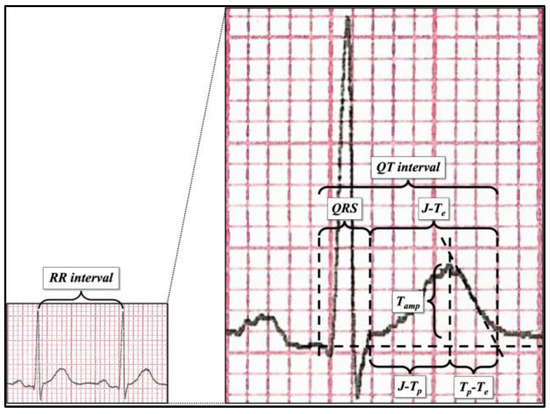
Figure 1.
ECG parameter measurement after 400% magnification.
Table 2.
Input feature set description.
2.3. Neural Networks
Neural networks are a set of algorithms modeled on human brain functions, designed to recognize patterns, i.e., the relationships, between the input and the output (target) signals [42]. In this work, two complementary approaches (human-engineered features vs automatic feature extraction) were tested to perform SQTS risk stratification. In the former scenario, cardiologists measured the features reported in Table 2 and this set was then fed to a shallow learning model, while in the latter case, ECG scans were fed directly to the Vision Transformer without any prior feature extraction phase. Human-engineered features have a direct, clear, medical explanation; for example, the R-R interval refers to the time between two heartbeats. However, the performance of a shallow neural network is highly affected by the input feature choice; since SQTS risk stratification is still an open problem, feature selection is not straightforward. On the other side, Deep Learning models are able to automatically extract the most significant features from the training input images and, therefore, cannot be biased by human-based feature selection. However, they act as a black box, which means they cannot provide any medical explanation of a good risk-stratification performance. It is worth mentioning that, given the limited size of the input dataset, it is probable that a shallow neural network would work better than Deep Learning models.
There are pros and cons in both scenarios; however, given the above, both approaches are complementary and worthy to be explored in an experimental setting.
2.3.1. Shallow Neural Networks: Human-Engineered Features
In a standard multi-layer perceptron (MLP) configuration, the input layer is made of a set of units (neurons), one per each feature, which work as an entry point to the neural network. Indeed, this layer consists of passive nodes, which do not modify the input but only transmit the information to each neuron of the subsequent layer (also known as fully connected). The hidden layer has an arbitrary number of neurons, which depends on the complexity of the problem at hand. Each hidden node combines the information received from each unit of the input layer to achieve a complex representation of the phenomenon under investigation. For this purpose, a non-linear activation function is employed, such as the hyperbolic tangent sigmoid. Finally, the output layer yields the classification of input data by means of the softmax function [43].
Due to the dataset size and the use of human-engineered features, it was chosen to use a shallow learning model. For this purpose, a feed-forward fully connected neural network with one hidden layer was designed. Different hidden-layer sizes were tested to evaluate the corresponding network classification performance; the best performing architecture had 30 and 1 neurons in the hidden and output layers, respectively, while the input layer size depends on the experiment (i.e., on the size of the input feature set). Aside from achieving superior performance, such configuration has a reduced capacity due to the lower number of neurons in the hidden layer. This feature can help prevent overfitting, which is likely to occur when analyzing such small datasets, threatening to invalidate the final results. Hidden units were equipped with hyperbolic tangent sigmoid transfer function, while the output layer used softmax to yield classification. The network training was performed using the scaled conjugate gradient (SCG) [44] technique to minimize the cross-entropy error function.
2.3.2. Shallow Neural Networks: Signals
A basic multi-layer perceptron was also fed with ECG signals extracted from the two-heartbeat image crops, which are detailed in the next sections. A signal extraction tool [45] was used, yielding 500-sample numerical signals for precordial leads (V1 to V3, since leads V4 to V6 were too noisy to be digitized on several images). This process was remarkably complicated and time-consuming. An example of an extracted numerical ECG signal is shown in Figure 2.
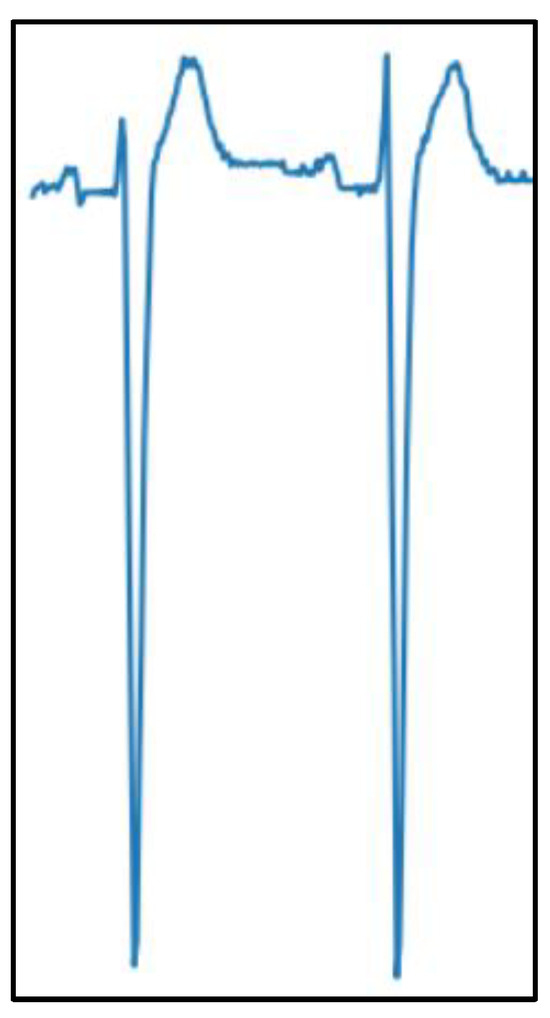
Figure 2.
Example of a digitized ECG signal extracted from a scanned image.
Several configurations for the neural network were tested; the best-performing one had 50 neurons in the hidden layer and 1 neuron in the output layer. The same considerations for the feature approach apply for this case.
2.3.3. Deep Learning Models: Convolutional Neural Networks
Despite being arguably surpassed by more recent models, convolutional neural networks (CNNs) are still the most common deep learning models for computer vision applications. CNNs apply different kernels over the input image in order to extract relevant features [46]. Stacking several layers, each one with a different kernel in charge of capturing a specific aspect of the picture, eventually allows the network to collect enough information to execute tasks like classification, segmentation, object detection, and the like.
CNN architectures deployed for this work included EfficientNetV2S, MobileNetV3, and ConvNextTiny [47,48,49], together with a 1-D CNN applied to numerical signals extracted from the images. Apparently, this approach did not yield the expected results, as detailed in the next sections.
2.3.4. Deep Learning Models: Vision Transformer and Swin Transformer
A different type of approach is offered by the Vision Transformer (or ViT), a deep neural network designed as a “computer vision version” of the original Transformer [50,51].
This architecture processes images by dividing them into equally sized patches, which are subsequently embedded and fed to the transformer. The embedding process also accounts for patch position within the image, thus retaining the positional information of each patch. The resulting vector is then processed inside the Transformer encoder by blocks called heads, which exploit the attention mechanism [52] to evaluate the information associated with each patch and how these “patches of information” are related to each other. Multiple heads perform these operations at once, allowing the network to gather knowledge about the global context of the picture. The encoder output is then fed to a multi-layer perceptron to classify the image on the basis of the information that the network was able to extract from it.
The stages of the Vision Transformer in image analysis are in many ways similar to what the human eye and brain do when looking at a picture, trying to grasp its meaning by merging information coming from details and knowledge gathered from the global picture, providing a tool that is able to extract features autonomously. Conversely, shallow learning models require ECG features as inputs to the network, thus implying the necessity to gather medical knowledge about the topic before network deployment.
A different version of the Vision Transformer, called Shifted Window Transformer (Swin Transformer) was developed in an attempt to make the basic ViT architecture better suited to vision tasks [53]. In fact, visual entities can undergo large variations, and image pixels can have significant resolution when compared to words in text. In order to overcome these issues, the Swin Transformer’s hierarchical architecture can adapt to different scales, and its computational complexity varies linearly with image size.
This model was applied to ECG images to assess performance against the Vision Transformer. Both Vision and Swin Transformers were pretrained on the ImageNet database [54] and fine-tuned on scanned ECG images. In addition, a 1-D version of the original Transformer encoder was applied to numerical signals extracted from the images.
2.3.5. Deep Learning Models: Capsule Neural Networks
Capsule neural networks (CapsNets) were designed to overcome some of CNNs’ main limitations, like lacking the capability to preserve spatial relationships among image elements [55]. In fact, to mention an “infamous” example, a CNN would typically identify a human face even when its elements—e.g., nose, mouth, eyes—were misplaced with respect to where they were expected to lie. With the introduction of capsule modules and dynamic routing, these neural models are able to capture the orientation of parts within an image.
2.3.6. Logistic Regression
One of the most common machine learning algorithms, logistic regression fits input data along a sigmoid function, assigning it to different classes according to where itlies along the function plot [56]. This classifier can be fed with images to perform classification, and in this case, it was applied to scanned ECG images.
2.4. Data Pre-Processing
The input dataset was pre-processed to enhance network training and avoid overfitting.
In the case of the shallow learning model, to reduce noise in the data and avoid bias in the network training, data were statistically normalized (z score) to make the network able to intrinsically determine the importance of each input feature for classification. Indeed, without this step, it would have been possible that some features masked some others, preventing the network from understanding the real contribution of each input attribute to SQTS risk stratification.
On the other hand, for the deep learning models, images were initially cropped to remove all the elements in the bordering part that did not strictly belong to an ECG chart. These elements are usually accompanying information (e.g., annotations) and are considered to carry no relevant data for the given task. Yet, if not removed, their information content could erroneously be marked as noteworthy by the model, thus introducing unwanted biases in classification. Figure 3 shows an example of an ECG image before and after the initial cropping.
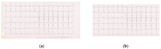
Figure 3.
(a) ECG image before cropping; (b) ECG image after cropping.
In order to try and isolate possible elements of the image carrying more information, images were later cropped to contain only two heartbeats, leading to two additional versions of the dataset: one containing two-heartbeat crops for each precordial lead (e.g.,: V1 only, V2 only, and so on, see Figure 4) and another one containing all two-heartbeat crops for all precordial leads (which are considered to hold more information than peripheral leads with respect to SQTS diagnosis).
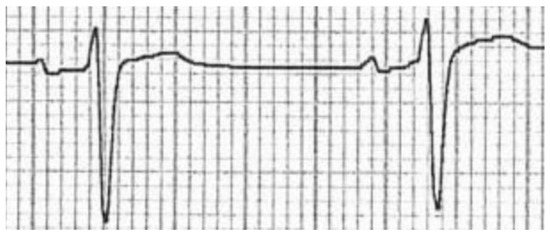
Figure 4.
Two-heartbeat crop of a single precordial lead from a scanned image.
Subsequently, data augmentation techniques were implemented for all deep learning models in order to help the network achieve better results during training. In particular, input images went through the following stages, undergoing the RandAugment method for image augmentation [57]: cropping at center; normalizing; horizontal flipping with a 50% probability of rotation occurring; random cropping and resizing; final resizing to the initial size. This process was especially necessary to try to level out the strong data imbalance between the two classes, which would otherwise lead to a penalization of the model’s generalization capabilities.
Another approach was the extraction of numerical signals from the two-heartbeat crops of leads V1, V2, and V3, with the purpose of trying to retrieve the information retained in the original ECG signals that were acquired by the time the data were collected. This was achieved by exploiting the specific tool mentioned previously in Section 2.3.2.
For all AI models, both the input and target sets were randomly divided into three sets as follows: 70% for training, 10% to validate that the network is generalizing and to stop training before overfitting, and the remaining 20% to independently test the network classification performance. To ensure the input data distribution (i.e., the amount of non-event/event cases) was preserved in the three sets, the random division was performed separately for non-event and event subsets.
2.5. Classification Metrics
Classification accuracy was estimated by analyzing the confusion matrices and the associated ROC curve. The former, shown in Figure 5, measures the number of times the network correctly classified the input; in this sense, it yields an estimate of how well a single class (negative/positive), i.e., a medical condition (non-event/event), was understood by the neural model. The rows and the columns correspond to the actual (i.e., target) and predicted classes, respectively. The diagonal cells correspond to the true observations (true positive and true negative) correctly classified, while the off-diagonal cells correspond to the false observations (false positive and false negative) incorrectly classified.
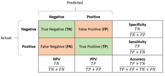
Figure 5.
Confusion matrix example: rows yield the real (actual) labels, columns the predicted ones, i.e., the network outputs.
To better analyze the network performance, five advanced classification metrics can be derived from the confusion matrix:
- Sensitivity, also referred to as True Positive Rate or Recall, measures the percentage of positive examples correctly labelled as positive by the classifier. In medicine, highly sensitive tests are generally used for screening purposes due to their ability to rule out the disease/event occurrence.
- Specificity, also known as True Negative Rate, measures the percentage of negative examples correctly labelled as negative by the classifier. In medicine, highly specific tests are typically used for confirmation purposes due to their ability to rule in the disease/event occurrence.
- Positive predictive value (PPV), also known as Precision, is the ratio between the total number of correctly classified positive examples and the total number of predicted positive examples. It yields the correctness achieved in positive prediction, which means it measures the likelihood that an event will truly occur given the corresponding network’s positive outcome.
- Negative predictive value (NPV) is the ratio between the total number of correctly classified negative examples and the total number of predicted negative examples. It yields the correctness achieved in negative prediction, which means it measures the likelihood that an event will truly not occur given the corresponding network’s negative outcome.
- Accuracy refers to the percentage of correct predictions. It is an average measure of the network quality.
- F1 Score is the harmonic mean of PPV and sensitivity. It is better suited than accuracy for unbalanced datasets.
Although accuracy provides a single global measure of the classification quality, it is just a mean value of the network performances. In contrast, the area under the ROC curve (AUC) yields a more precise measure (the higher the better) of the predictive accuracy because it represents the probability that a randomly chosen positive sample is ranked higher than a corresponding negative one.
3. Results
The classification ability of the proposed shallow learning model was tested on different input configurations, i.e., different input human-engineered feature sets, to study which features were the most relevant to correctly discriminating subjects who will have an event from those who will not. In this sense, the importance of the QT interval and that of the T wave in distinguishing the two classes (i.e., non-event/event) were investigated. Therefore, the experiments could be grouped into five categories as per Table 3:
Table 3.
Input dataset taxonomy.
- QT: only the QT-related features were considered;
- Twave: only the T-wave features were considered;
- QT + Twave: both the QT-related and T-wave features were considered;
- Twave ext: T-wave features were considered together with their Bazett-corrected values;
- All: all input features were considered.
To assess the network classification performances, sensitivity, specificity, PPV, NPV, and accuracy were evaluated. The results for the test set (see Table 4), which checked the ability of the models to perform on new and previously unseen samples, can be summarized as follows:
Table 4.
Shallow network (human-engineered features) classification performances: sensitivity, specificity, PPV, NPV, accuracy, F1 score. Values are in percentages. The highest values for each metric are highlighted in bold.
- Sensitivity: this was generally low in all configurations, with a maximum value of 63.6% in the Twave input configuration and a minimum of 36.4% in the All configuration.
- Specificity: this metric was generally high across all the different explored input configurations, with values ranging from 85% (Twave) to 95% (QT, Twave ext, and All).
- PPV and NPV: these two metrics did not show optimal values in any of the proposed input configurations; in particular, PPV showed better results compared with NPV (maximum PPV: 83.3% in QT and Twave ext; maximum NPV: 81% in Twave).
- Accuracy: this evaluation metric was generally suboptimal across all the evaluated configurations, with all the configurations showing 77.4% accuracy with only the exception of the All input configuration, which showed slightly reduced accuracy in the test set (74.2%).
- F1 Score: this evaluation metric was generally suboptimal across all the evaluated configurations, with the Twave configuration reaching the highest value of 66.6 and QT + Twave showing roughly the same performance (63.1).
Finally, Table 5 reports the AUC values for the five evaluated feature sets. While the training-set AUCs are generally satisfying, the same cannot be said for the test-set AUCs. In fact, as can be appreciated, AUC values drop to poor values (AUC < 0.60) or just acceptable values (AUC 0.60–0.70) in all the configurations, except for the QT + Twave configuration, which also presents a good AUC in the testing set (0.81).
Table 5.
Shallow network (human-engineered features) classification performances: AUC.
Table 6 and Table 7 summarize the results for the other approaches (signal and image analysis). Reported metrics are the test accuracy and the AUC scores obtained by feeding the networks with signals and single lead images. Results are quite similar, regardless of the input type and/or the network architecture: apparently, none of those methods was able to capture any significant difference between the two categories, interpreting every input as a case without an SCD event.
Table 6.
Signal classification approach performances: test accuracy (percentage) and AUC.
Table 7.
Image classification approach performances: test accuracy (percentage) and AUC.
Comparison with Classical Machine Learning Algorithms
Since the dataset is very small (104 samples and at most 13 features), the one-hidden-layer perceptron is not guaranteed to perform better than other classical ML models. Therefore, to better assess the quality of the proposed shallow learning model, an additional comparison was performed with classical machine learning algorithms including logistic regression [58], decision tree [59], boosted decision tree [59], bagged decision tree [60], support vector machine (SVM) [59], and k-nearest neighbors (KNN) [61]. Also, a PCA feature-selection technique [62] was employed as preprocessing, retaining 90% of the overall explained variance, to see whether reducing the input space would imply an improvement in the classification [63].
Table 8 yields the results for the test set, where different settings of these methods are reported. In more detail:
Table 8.
Accuracy classification performances of state-of-the-art ML methods for the five input configurations, with or without PCA data preprocessing (90% of explained variance retained). Values are in percentages. The highest values in each column are highlighted in bold.
- Fine tree, medium tree, coarse tree: decision trees with Gini’s diversity index as split criterion and a maximum number of splits equal to 100, 20, 4, for fine, medium, and coarse trees, respectively.
- Boosted decision tree: ensemble of decision trees using the AdaBoost algorithm (maximum number of splits: 20, number of learners: 30, learning rate: 0.1).
- Bagged decision tree: ensemble of decision trees [59] using Bag algorithm (maximum number of splits: 72, number of learners: 30).
- SVMs: support vector machines [59] with different kernel functions, i.e., linear, quadratic, cubic, Gaussian with kernel scale equal to 0.5 (fine Gaussian), 2 (medium Gaussian), and 8 (coarse Gaussian).
- Fine KNN, medium KNN, coarse KNN: k-nearest neighbors algorithm using Euclidean distance as the metric and numbers of neighbors equal to 1, 10, 100, for fine, medium, and coarse KNN, respectively.
- Cosine KNN: k-nearest neighbor algorithm using a number of neighbors equal to 10 and cosine distance as the metric.
- Cubic KNN: k-nearest neighbor algorithm using a number of neighbors equal to 10 and Minkowsky distance as the metric.
Despite some of these methods showing promising results (i.e., 71.0% accuracy), none reached the same accuracy as the shallow learning (i.e., 77.4%). Only the coarse tree with PCA arrived at 74.2% accuracy, still below that of the shallow learning. The results for PCA behavior are not conclusive, since in some cases it improved performances, while in some other cases it worsened them, even for the same technique; as an example, see medium tree vs coarse tree, or quadratic SVM vs cubic SVM.
4. Discussion
SQTS is an inherited channelopathy related to increased risk of SCD. SCD is often the first symptomatic presentation, demanding an important effort to better stratify the risk of arrhythmia in patients who are still asymptomatic at medical evaluation. Until now, risk stratification in asymptomatic patients has been unsatisfactory. To our knowledge, this is the first work using an AI-based approach to analyze ECGs in patients with SQTS in order to refine arrhythmia risk stratification. In this study, we used two different AI-based approaches to this purpose: the first approach requires manual feature extraction from the ECG, which is used as input for shallow learning models; other approaches directly use the scanned ECG image or the signal extracted from it as input, automatically performing feature extraction. The main findings are summarized in the following.
Shallow learning models based on different configurations of manually extracted (human-engineered) ECG features achieved suboptimal performance, in particular regarding the NPV, which never exceeded 81%; this is clinically relevant, since it means 2 out of 10 patients with an event were incorrectly classified in the non-event group, potentially leading to under-treatment.
All other approaches did not seem to grasp any significant difference between the two classes and ended up considering each input as a case with no SCD event. There are several possible factors that might have influenced such results:
- Scanned ECG images were extremely different from each other, in terms of resolution, format, color, and background grid color, and most of them suffered from noisy, poor quality; this hindered the possibility of developing a consistent preprocessing procedure that could work efficiently on all dataset images.
- Dataset cardinality was particularly low; this could represent an obstacle for some of the deep learning models chosen, for both the image and the signal approaches. In fact, such architectures often contain a vast number of parameters, and are usually trained on very large datasets.
- Image cropping was performed manually, both for lead isolation and signal digitization; this might have introduced some errors due to the lack of specific methods and criteria for accurate and precise definition of the cropping area.
- The image and signal approaches were conceived to be specular to the feature approach: tested models were supposed to automatically extract relevant features in an unbiased manner, potentially uncovering aspects of the ECG chart that can enrich the knowledge about SQTS and unveiling elements that can hint at an increased risk of an SCD event. Therefore, this methodology cannot leverage any a priori information that could steer the feature search towards a specific direction.
These results suggest that AI-based ECG analysis, in particular using the features approach, might help in refining risk stratification in SQTS patients, supporting clinical decision making in a context where incorrect risk appraisal might translate into the death of young and otherwise healthy individuals. A refined risk stratification means that the clinician may offer the patients the most appropriate treatment to prevent SCD, including cardiac devices. Implantable cardioverter defibrillators (ICDs) still represent the mainstay of treatment for patients with SQTS who are survivors of SCD or have documented spontaneous sustained VT [64], despite significant risk of device-related complications, such as inappropriate shocks (33%), device-related infection (10%), lead failure and fracture (21%), and psychological distress (3.5%) [65,66]. In this sense, better risk stratification might lead not only to earlier adoption of life-saving therapy for patients deemed at higher risk of SCD but also to avoiding implantation of ICDs in low-risk patients, potentially sparing the risk of device-related complications.
Study Limits
The present work has some limitations, which need to be addressed. First, we acknowledge that the number of patients was limited; however, it should be borne in mind that SQTS is a rare disease, and this constitutes the widest cohort of SQTS patients published so far. Given the limited quantity of ECGSs, it was not possible to refine the analysis into different subgroups, since the results would not have been significant from a statistical point of view.
For the shallow learning model, ECG features were not automatically extracted, but manually calculated by three experienced cardiologists (albeit with 400% magnification to minimize measurement errors), which is prone to errors in manual measurement. Moreover, the study suffers from an implicit bias in terms of the selected features set: although the thirteen features were selected based on the current medical knowledge, they may not be the most relevant to perform SQTS risk stratification. Further studies with different feature sets should be considered. Future works will investigate different methods of feature selection, e.g., L1 regularization, and deepen the relationships among the features and the classification performances.
Finally, to increase generalizability and better assess their reliability, the results presented in this study will be verified in an external SQTS population originating from different regions or medical centers.
5. Conclusions
Short QT syndrome is an inherited channelopathy linked with an increased risk of SCD in young and otherwise healthy individuals. Clinical presentation of patients affected by SQTS is highly heterogeneous, with SCD often being the first clinical presentation, and risk stratification is particularly challenging in asymptomatic subjects.
The analysis of ECGs from SQTS patients with the aid of neural networks shows promising results in terms of discriminating between subjects with and without documented arrhythmic events. This could pave the way for refined ECG-based risk stratification in this group of patients, potentially helping in saving the lives of young and otherwise healthy individuals, such as in the initial study performed on Brugada syndrome [59].
Future studies should focus on automatic calculation of the features from digital ECG recordings (either using raw digital ECG data or digitized data from paper-based ECGs). This will guarantee increased reproducibility compared with manual extraction of relevant ECG features. In addition, other deep learning models assessing the whole raw digital ECG signal and/or ECG images should also be explored and should be compared with other architectures. As an example, images will be converted to the frequency domain to apply frequency-domain filters or Wiener filters for noise reduction, so that it will be possible to provide cleaner input to vision-based deep learning models. In parallel, authors will continue to collect SQTS ECGs of subjects who have developed an event, to increase the cardinality of the dataset and further validate the proposed approach; for this purpose, it will probably be necessary to include different cohorts originating from different regions and medical centers. Finally, data augmentation by means of GANs will be explored to increase the quantity of ECG images and, thus, the classification performance.
Author Contributions
Conceptualization, F.G., E.P. and V.R.; methodology, V.R., E.P. and S.C.; software, V.R. and S.C.; validation, V.R., E.P. and S.C.; formal analysis, P.M. (Pierre Meynet), V.R., P.M. (Philippe Maury) and S.C.; investigation, F.G., C.G. and P.M. (Pierre Meynet); resources, E.P., F.G. and C.G.; data curation, P.M. (Pierre Meynet), P.M. (Philippe Maury) and C.G.; writing—original draft preparation, V.R., S.C., P.M. (Pierre Meynet) and C.G.; writing—review and editing, C.G., V.R., P.M. (Philippe Maury) and F.G.; visualization, S.C. and V.R.; supervision, F.G., E.P. and C.G.; project administration, E.P. and V.R.; funding acquisition, E.P., V.R. and C.G. All authors have read and agreed to the published version of the manuscript.
Funding
This research has been partly funded by the BrS-AI-ECG project of the Italian Ministry of Foreign Affairs and International Cooperation. Dr. Randazzo also acknowledges funding from the research contract no. 32-G-13427-2 (DM 1062/2021) funded within the Programma Operativo Nazionale (PON) Ricerca e Innovazione of the Italian Ministry of University and Research.
Institutional Review Board Statement
The study was conducted according to the guidelines of the Declaration of Helsinki and approved by the Institutional Review Board of Città della Salute e della Scienza Hospital, Turin, Italy (Protocol code: 248/2017, date of approval: 22 February 2017).
Informed Consent Statement
Informed consent was obtained from all subjects involved in the study.
Data Availability Statement
The data presented in this study are available on request from the corresponding author.
Acknowledgments
Authors thank Annunziata Paviglianiti and Andrea Saglietto for the initial support.
Conflicts of Interest
The authors declare no conflict of interest.
References
- Gussak, I.; Brugada, P.; Brugada, J.; Wright, R.S.; Kopecky, S.L.; Chaitman, B.R.; Bjerregaard, P. Idiopathic Short QT Interval:A New Clinical Syndrome? Cardiology 2000, 94, 99–102. [Google Scholar] [CrossRef]
- Gaita, F.; Giustetto, C.; Bianchi, F.; Wolpert, C.; Schimpf, R.; Riccardi, R.; Grossi, S.; Richiardi, E.; Borggrefe, M. Short QT Syndrome: A Familial Cause of Sudden Death. Circulation 2003, 108, 965–970. [Google Scholar] [CrossRef] [PubMed]
- Brugada, R.; Hong, K.; Dumaine, R.; Cordeiro, J.; Gaita, F.; Borggrefe, M.; Menendez, T.M.; Brugada, J.; Pollevick, G.D.; Wolpert, C.; et al. Sudden Death Associated With Short-QT Syndrome Linked to Mutations in HERG. Circulation 2004, 109, 30–35. [Google Scholar] [CrossRef] [PubMed]
- Bellocq, C.; van Ginneken, A.C.G.; Bezzina, C.R.; Alders, M.; Escande, D.; Mannens, M.M.A.M.; Baró, I.; Wilde, A.A.M. Mutation in the KCNQ1 Gene Leading to the Short QT-Interval Syndrome. Circulation 2004, 109, 2394–2397. [Google Scholar] [CrossRef] [PubMed]
- Priori, S.G.; Pandit, S.V.; Rivolta, I.; Berenfeld, O.; Ronchetti, E.; Dhamoon, A.; Napolitano, C.; Anumonwo, J.; di Barletta, M.R.; Gudapakkam, S.; et al. A Novel Form of Short QT Syndrome (SQT3) Is Caused by a Mutation in the KCNJ2 Gene. Circ. Res. 2005, 96, 800–807. [Google Scholar] [CrossRef]
- Walsh, R.; Adler, A.; Amin, A.S.; Abiusi, E.; Care, M.; Bikker, H.; Amenta, S.; Feilotter, H.; Nannenberg, E.A.; Mazzarotto, F.; et al. Evaluation of Gene Validity for CPVT and Short QT Syndrome in Sudden Arrhythmic Death. Eur. Heart J. 2022, 43, 1500–1510. [Google Scholar] [CrossRef]
- Mazzanti, A.; Kanthan, A.; Monteforte, N.; Memmi, M.; Bloise, R.; Novelli, V.; Miceli, C.; O’Rourke, S.; Borio, G.; Zienciuk-Krajka, A.; et al. Novel Insight Into the Natural History of Short QT Syndrome. J. Am. Coll. Cardiol. 2014, 63, 1300–1308. [Google Scholar] [CrossRef]
- Zeppenfeld, K.; Tfelt-Hansen, J.; de Riva, M.; Winkel, B.G.; Behr, E.R.; Blom, N.A.; Charron, P.; Corrado, D.; Dagres, N.; de Chillou, C.; et al. 2022 ESC Guidelines for the Management of Patients with Ventricular Arrhythmias and the Prevention of Sudden Cardiac Death. Eur. Heart J. 2022, 43, 3997–4126. [Google Scholar] [CrossRef] [PubMed]
- Giustetto, C.; Schimpf, R.; Mazzanti, A.; Scrocco, C.; Maury, P.; Anttonen, O.; Probst, V.; Blanc, J.-J.; Sbragia, P.; Dalmasso, P.; et al. Long-Term Follow-Up of Patients With Short QT Syndrome. J. Am. Coll. Cardiol. 2011, 58, 587–595. [Google Scholar] [CrossRef]
- Rudic, B.; Schimpf, R.; Borggrefe, M. Short QT Syndrome—Review of Diagnosis and Treatment. Arrhythm. Electrophysiol. Rev. 2014, 3, 76–79. [Google Scholar] [CrossRef] [PubMed]
- Anttonen, O.; Junttila, M.J.; Maury, P.; Schimpf, R.; Wolpert, C.; Borggrefe, M.; Giustetto, C.; Gaita, F.; Sacher, F.; Haïssaguerre, M.; et al. Differences in Twelve-Lead Electrocardiogram between Symptomatic and Asymptomatic Subjects with Short QT Interval. Heart Rhythm. 2009, 6, 267–271. [Google Scholar] [CrossRef]
- Tülümen, E.; Giustetto, C.; Wolpert, C.; Maury, P.; Anttonen, O.; Probst, V.; Blanc, J.-J.; Sbragia, P.; Scrocco, C.; Rudic, B.; et al. PQ Segment Depression in Patients with Short QT Syndrome: A Novel Marker for Diagnosing Short QT Syndrome? Heart Rhythm. 2014, 11, 1024–1030. [Google Scholar] [CrossRef] [PubMed]
- Topol, E.J. High-Performance Medicine: The Convergence of Human and Artificial Intelligence. Nat. Med. 2019, 25, 44–56. [Google Scholar] [CrossRef]
- Valente, F.; Henriques, J.; Paredes, S.; Rocha, T.; de Carvalho, P.; Morais, J. A New Approach for Interpretability and Reliability in Clinical Risk Prediction: Acute Coronary Syndrome Scenario. Artif. Intell. Med. 2021, 117, 102113. [Google Scholar] [CrossRef]
- Alfieri, F.; Ancona, A.; Tripepi, G.; Crosetto, D.; Randazzo, V.; Paviglianiti, A.; Pasero, E.; Vecchi, L.; Cauda, V.; Fagugli, R.M. A Deep-Learning Model to Continuously Predict Severe Acute Kidney Injury Based on Urine Output Changes in Critically Ill Patients. J. Nephrol. 2021, 34, 1875–1886. [Google Scholar] [CrossRef]
- Roberti, I.; Lovino, M.; Di Cataldo, S.; Ficarra, E.; Urgese, G. Exploiting Gene Expression Profiles For The Automated Prediction Of Connectivity Between Brain Regions. Int. J. Mol. Sci. 2019, 20, 2035. [Google Scholar] [CrossRef] [PubMed]
- de Siqueira, V.S.; Borges, M.M.; Furtado, R.G.; Dourado, C.N.; da Costa, R.M. Artificial Intelligence Applied to Support Medical Decisions for the Automatic Analysis of Echocardiogram Images: A Systematic Review. Artif. Intell. Med. 2021, 120, 102165. [Google Scholar] [CrossRef]
- Siontis, K.C.; Noseworthy, P.A.; Attia, Z.I.; Friedman, P.A. Artificial Intelligence-Enhanced Electrocardiography in Cardiovascular Disease Management. Nat. Rev. Cardiol. 2021, 18, 465–478. [Google Scholar] [CrossRef] [PubMed]
- Attia, Z.I.; Noseworthy, P.A.; Lopez-Jimenez, F.; Asirvatham, S.J.; Deshmukh, A.J.; Gersh, B.J.; Carter, R.E.; Yao, X.; Rabinstein, A.A.; Erickson, B.J.; et al. An Artificial Intelligence-Enabled ECG Algorithm for the Identification of Patients with Atrial Fibrillation during Sinus Rhythm: A Retrospective Analysis of Outcome Prediction. Lancet 2019, 394, 861–867. [Google Scholar] [CrossRef] [PubMed]
- Baker, S.; Xiang, W.; Atkinson, I. A Hybrid Neural Network for Continuous and Non-Invasive Estimation of Blood Pressure from Raw Electrocardiogram and Photoplethysmogram Waveforms. Comput. Methods Programs Biomed. 2021, 207, 106191. [Google Scholar] [CrossRef]
- Paviglianiti, A.; Randazzo, V.; Villata, S.; Cirrincione, G.; Pasero, E. A Comparison of Deep Learning Techniques for Arterial Blood Pressure Prediction. Cogn. Comput. 2021, 14, 1689–1710. [Google Scholar] [CrossRef]
- Paviglianiti, A.; Randazzo, V.; Cirrincione, G.; Pasero, E. Double Channel Neural Non Invasive Blood Pressure Prediction. In Proceedings of the Intelligent Computing Theories and Application; Huang, D.-S., Bevilacqua, V., Hussain, A., Eds.; Springer International Publishing: Cham, Switzerland, 2020; pp. 160–171. [Google Scholar]
- Paviglianiti, A.; Randazzo, V.; Cirrincione, G.; Pasero, E. Neural Recurrent Approches to Noninvasive Blood Pressure Estimation. In Proceedings of the 2020 International Joint Conference on Neural Networks (IJCNN), Glasgow, UK, 15–16 July 2020; pp. 1–7. [Google Scholar]
- Paviglianiti, A.; Randazzo, V.; Pasero, E.; Vallan, A. Noninvasive Arterial Blood Pressure Estimation Using ABPNet and VITAL-ECG. In Proceedings of the 2020 IEEE International Instrumentation and Measurement Technology Conference (I2MTC), Dubrovnik, Croatia, 25–29 May 2020; pp. 1–5. [Google Scholar]
- Attia, Z.I.; Friedman, P.A.; Noseworthy, P.A.; Lopez-Jimenez, F.; Ladewig, D.J.; Satam, G.; Pellikka, P.A.; Munger, T.M.; Asirvatham, S.J.; Scott, C.G.; et al. Age and Sex Estimation Using Artificial Intelligence From Standard 12-Lead ECGs. Circ. Arrhythmia Electrophysiol. 2019, 12, e007284. [Google Scholar] [CrossRef] [PubMed]
- Attia, Z.I.; Kapa, S.; Lopez-Jimenez, F.; McKie, P.M.; Ladewig, D.J.; Satam, G.; Pellikka, P.A.; Enriquez-Sarano, M.; Noseworthy, P.A.; Munger, T.M.; et al. Screening for Cardiac Contractile Dysfunction Using an Artificial Intelligence–Enabled Electrocardiogram. Nat. Med. 2019, 25, 70–74. [Google Scholar] [CrossRef]
- Galloway, C.D.; Valys, A.V.; Shreibati, J.B.; Treiman, D.L.; Petterson, F.L.; Gundotra, V.P.; Albert, D.E.; Attia, Z.I.; Carter, R.E.; Asirvatham, S.J.; et al. Development and Validation of a Deep-Learning Model to Screen for Hyperkalemia From the Electrocardiogram. JAMA Cardiol. 2019, 4, 428–436. [Google Scholar] [CrossRef]
- Wang, J.; Qiao, X.; Liu, C.; Wang, X.; Liu, Y.; Yao, L.; Zhang, H. Automated ECG Classification Using a Non-Local Convolutional Block Attention Module. Comput. Methods Programs Biomed. 2021, 203, 106006. [Google Scholar] [CrossRef]
- Asl, B.M.; Setarehdan, S.K.; Mohebbi, M. Support Vector Machine-Based Arrhythmia Classification Using Reduced Features of Heart Rate Variability Signal. Artif. Intell. Med. 2008, 44, 51–64. [Google Scholar] [CrossRef] [PubMed]
- Ferretti, J.; Randazzo, V.; Cirrincione, G.; Pasero, E. 1-D Convolutional Neural Network for ECG Arrhythmia Classification. In Progresses in Artificial Intelligence and Neural Systems; Esposito, A., Faundez-Zanuy, M., Morabito, F.C., Pasero, E., Eds.; Smart Innovation, Systems and Technologies; Springer: Singapore, 2021; pp. 269–279. ISBN 9789811550935. [Google Scholar]
- Rahman, Q.A.; Tereshchenko, L.G.; Kongkatong, M.; Abraham, T.; Abraham, M.R.; Shatkay, H. Utilizing ECG-Based Heartbeat Classification for Hypertrophic Cardiomyopathy Identification. IEEE Trans. NanoBiosci. 2015, 14, 505–512. [Google Scholar] [CrossRef] [PubMed]
- Hassan, M.R.; Huda, S.; Hassan, M.M.; Abawajy, J.; Alsanad, A.; Fortino, G. Early Detection of Cardiovascular Autonomic Neuropathy: A Multi-Class Classification Model Based on Feature Selection and Deep Learning Feature Fusion. Inf. Fusion 2022, 77, 70–80. [Google Scholar] [CrossRef]
- Sahli Costabal, F.; Matsuno, K.; Yao, J.; Perdikaris, P.; Kuhl, E. Machine Learning in Drug Development: Characterizing the Effect of 30 Drugs on the QT Interval Using Gaussian Process Regression, Sensitivity Analysis, and Uncertainty Quantification. Comput. Methods Appl. Mech. Eng. 2019, 348, 313–333. [Google Scholar] [CrossRef]
- Dai, H.; Hwang, H.-G.; Tseng, V.S. Convolutional Neural Network Based Automatic Screening Tool for Cardiovascular Diseases Using Different Intervals of ECG Signals. Comput. Methods Programs Biomed. 2021, 203, 106035. [Google Scholar] [CrossRef]
- Liu, H.; Zhao, Z.; Chen, X.; Yu, R.; She, Q. Using the VQ-VAE to Improve the Recognition of Abnormalities in Short-Duration 12-Lead Electrocardiogram Records. Comput. Methods Programs Biomed. 2020, 196, 105639. [Google Scholar] [CrossRef] [PubMed]
- Monedero, I. A Novel ECG Diagnostic System for the Detection of 13 Different Diseases. Eng. Appl. Artif. Intell. 2022, 107, 104536. [Google Scholar] [CrossRef]
- Green, M.; Björk, J.; Forberg, J.; Ekelund, U.; Edenbrandt, L.; Ohlsson, M. Comparison between Neural Networks and Multiple Logistic Regression to Predict Acute Coronary Syndrome in the Emergency Room. Artif. Intell. Med. 2006, 38, 305–318. [Google Scholar] [CrossRef]
- Ferretti, J.; Barbiero, P.; Randazzo, V.; Cirrincione, G.; Pasero, E. Towards Uncovering Feature Extraction from Temporal Signals in Deep CNN: The ECG Case Study. In Proceedings of the 2020 International Joint Conference on Neural Networks (IJCNN), Glasgow, UK, 19–24 July 2020; pp. 1–7. [Google Scholar] [CrossRef]
- Cirrincione, G.; Randazzo, V.; Pasero, E. A Neural Based Comparative Analysis for Feature Extraction from ECG Signals. In Neural Approaches to Dynamics of Signal Exchanges; Esposito, A., Faundez-Zanuy, M., Morabito, F.C., Pasero, E., Eds.; Smart Innovation, Systems and Technologies; Springer: Singapore, 2020; pp. 247–256. ISBN 9789811389504. [Google Scholar]
- Postema, P.G.; Wilde, A.A.M. The Measurement of the QT Interval. Curr. Cardiol. Rev. 2014, 10, 287–294. [Google Scholar] [CrossRef]
- Gaita, F.; Giustetto, C.; Bianchi, F.; Schimpf, R.; Haissaguerre, M.; Calò, L.; Brugada, R.; Antzelevitch, C.; Borggrefe, M.; Wolpert, C. Short QT Syndrome: Pharmacological Treatment. J. Am. Coll. Cardiol. 2004, 43, 1494–1499. [Google Scholar] [CrossRef] [PubMed]
- Zhang, Z. A Gentle Introduction to Artificial Neural Networks. Ann. Transl. Med. 2016, 4, 370. [Google Scholar] [CrossRef]
- Bishop, C.M.; Nasser, M.N. Pattern Recognition and Machine Learning; Springer: New York, NY, USA, 2006; Volume 6. [Google Scholar]
- Goodfellow, I.; Bengio, Y.; Courville, A. Back-Propagation and other Differentiation Algorithms; Deep Learning; MIT Press: Cambridge, MA, USA, 2016; pp. 200–220. [Google Scholar]
- Randazzo, V.; Puleo, E.; Paviglianiti, A.; Vallan, A.; Pasero, E. Development and Validation of an Algorithm for the Digitization of ECG Paper Images. Sensors 2022, 22, 7138. [Google Scholar] [CrossRef]
- Boser, B.; Denker, J.S.; Henderson, D.; Howard, R.E.; Hubbard, W.; Jackel, L.D.; Laboratories, H.Y.L.B.; Zhu, Z.; Cheng, J.; Zhao, Y.; et al. Backpropagation Applied to Handwritten Zip Code Recognition. Neural Comput. 1989, 1, 541–551. [Google Scholar] [CrossRef]
- Tan, M.; Le, Q.V. EfficientNetV2: Smaller Models and Fast Training. arXiv 2021, arXiv:2104.00298. [Google Scholar] [CrossRef]
- Howard, A.; Sandler, M.; Chen, B.; Wang, W.; Chen, L.-C.; Tan, M.; Chu, G.; Vasudevan, V.; Zhu, Y.; Pang, R.; et al. Searching for MobileNetV3. In Proceedings of the IEEE/CVF International Conference on Computer Vision (ICCV), Seoul, Republic of Korea, 27 October–2 November 2019; pp. 1314–1324. [Google Scholar] [CrossRef]
- Liu, Z.; Mao, H.; Wu, C.-Y.; Feichtenhofer, C.; Darrell, T.; Xie, S. A ConvNet for the 2020s. In Proceedings of the 2022 IEEE/CVF Conference on Computer Vision and Pattern Recognition (CVPR), New Orleans, LA, USA, 18–24 June 2022; pp. 11966–11976. [Google Scholar] [CrossRef]
- Vaswani, A.; Shazeer, N.; Parmar, N.; Uszkoreit, J.; Jones, L.; Gomez, A.N.; Kaiser, L.; Polosukhin, I. Attention Is All You Need. arXiv 2017, arXiv:1706.03762. [Google Scholar] [CrossRef]
- Dosovitskiy, A.; Beyer, L.; Kolesnikov, A.; Weissenborn, D.; Zhai, X.; Unterthiner, T.; Dehghani, M.; Minderer, M.; Heigold, G.; Gelly, S.; et al. An Image Is Worth 16x16 Words: Transformers for Image Recognition at Scale. arXiv 2020, arXiv:2010.11929. [Google Scholar] [CrossRef]
- Bahdanau, D.; Cho, K.; Bengio, Y. Neural Machine Translation by Jointly Learning to Align and Translate. arXiv 2014, arXiv:1409.0473. [Google Scholar] [CrossRef]
- Liu, Z.; Lin, Y.; Cao, Y.; Hu, H.; Wei, Y.; Zhang, Z.; Lin, S.; Guo, B. Swin Transformer: Hierarchical Vision Transformer using Shifted Windows. arXiv 2021, arXiv:2103.14030. [Google Scholar] [CrossRef]
- Deng, J.; Dong, W.; Socher, R.; Li, L.-J.; Li, K.; Fei-Fei, L. ImageNet: A large-scale hierarchical image database. In Proceedings of the 2009 IEEE Conference on Computer Vision and Pattern Recognition, Miami, FL, USA, 20–25 June 2009; pp. 248–255. [Google Scholar] [CrossRef]
- Sabour, S.; Frosst, N.; Hinton, G.E. Dynamic Routing Between Capsules. arXiv 2017, arXiv:1710.09829. [Google Scholar] [CrossRef]
- Tolles, J.; Meurer, W.J. Logistic Regression: Relating Patient Characteristics to Outcomes. JAMA 2016, 316, 533–534. [Google Scholar] [CrossRef] [PubMed]
- Cubuk, E.D.; Zoph, B.; Shlens, J.; Le, Q.V. RandAugment: Practical Automated Data Augmentation with a Reduced Search Space. arXiv 2019, arXiv:1909.13719. [Google Scholar] [CrossRef]
- LaValley, M.P. Logistic regression. Circulation 2008, 117, 2395–2399. [Google Scholar] [CrossRef]
- Randazzo, V.; Marchetti, G.; Giustetto, C.; Gugliermina, E.; Kumar, R.; Cirrincione, G.; Gaita, F.; Pasero, E. Learning-Based Approach to Predict Fatal Events in Brugada Syndrome. In Applications of Artificial Intelligence and Neural Systems to Data Science; Springer Nature: Singapore, 2023; pp. 63–72. [Google Scholar] [CrossRef]
- Netsanet, S.; Zhang, J.; Zheng, D. Bagged Decision Trees Based Scheme of Microgrid Protection Using Windowed Fast Fourier and Wavelet Transforms. Electronics 2018, 7, 61. [Google Scholar] [CrossRef]
- Samet, H. K-Nearest Neighbor Finding Using MaxNearestDist. IEEE Trans. Pattern Anal. Mach. Intell. 2008, 30, 243–252. [Google Scholar] [CrossRef]
- Randazzo, V.; Cirrincione, G.; Pasero, E. Shallow Neural Network for Biometrics from the ECG-WATCH. In Intelligent Computing Theories and Application; Huang, D.S., Bevilacqua, V., Hussain, A., Eds.; ICIC 2020. Lecture Notes in Computer Science; Springer: Cham, Switzerland, 2020; Volume 12463. [Google Scholar] [CrossRef]
- Lovino, M.; Randazzo, V.; Ciravegna, G.; Barbiero, P.; Ficarra, E.; Cirrincione, G. A survey on data integration for multi-omics sample clustering. Neurocomputing 2022, 488, 494–508. [Google Scholar] [CrossRef]
- Priori, S.G.; Blomström-Lundqvist, C.; Mazzanti, A.; Blom, N.; Borggrefe, M.; Camm, J.; Elliott, P.M.; Fitzsimons, D.; Hatala, R.; Hindricks, G.; et al. 2015 ESC Guidelines for the Management of Patients with Ventricular Arrhythmias and the Prevention of Sudden Cardiac Death: The Task Force for the Management of Patients with Ventricular Arrhythmias and the Prevention of Sudden Cardiac Death of the European Society of Cardiology (ESC)Endorsed by: Association for European Paediatric and Congenital Cardiology (AEPC). Eur. Heart J. 2015, 36, 2793–2867. [Google Scholar] [CrossRef] [PubMed]
- Schimpf, R.; Wolpert, C.; Bianchi, F.; Giustetto, C.; Gaita, F.; Bauersfeld, U.; Borggrefe, M. Congenital Short QT Syndrome and Implantable Cardioverter Defibrillator Treatment. J. Cardiovasc. Electrophysiol. 2003, 14, 1273–1277. [Google Scholar] [CrossRef] [PubMed]
- El-Battrawy, I.; Besler, J.; Ansari, U.; Liebe, V.; Schimpf, R.; Tülümen, E.; Rudic, B.; Lang, S.; Odening, K.; Cyganek, L.; et al. Long-Term Follow-up of Implantable Cardioverter-Defibrillators in Short QT Syndrome. Clin. Res. Cardiol. 2019, 108, 1140–1146. [Google Scholar] [CrossRef] [PubMed]
Disclaimer/Publisher’s Note: The statements, opinions and data contained in all publications are solely those of the individual author(s) and contributor(s) and not of MDPI and/or the editor(s). MDPI and/or the editor(s) disclaim responsibility for any injury to people or property resulting from any ideas, methods, instructions or products referred to in the content. |
© 2023 by the authors. Licensee MDPI, Basel, Switzerland. This article is an open access article distributed under the terms and conditions of the Creative Commons Attribution (CC BY) license (https://creativecommons.org/licenses/by/4.0/).