Abstract
The rapid advancement of climate change and global warming have widespread impacts on society, including ecosystems, water security, food production, health, and infrastructure. To achieve significant global emission reductions, approximately 74% is expected to come from cutting carbon dioxide (CO) emissions in energy supply and demand. Carbon Capture and Storage (CCS) has attained global recognition as a preeminent approach for the mitigation of atmospheric carbon dioxide levels, primarily by means of capturing and storing CO emissions originating from fossil fuel systems. Currently, geological models for storage location determination in CCS rely on limited sampling data from borehole surveys, which poses accuracy challenges. To tackle this challenge, our research project focuses on analyzing exposed rock formations, known as outcrops, with the goal of identifying the most effective backbone networks for classifying various strata types in outcrop images. We leverage deep learning-based outcrop semantic segmentation techniques using hybrid backbone networks, named OutcropHyBNet, to achieve accurate and efficient lithological classification, while considering texture features and without compromising computational efficiency. We conducted accuracy comparisons using publicly available benchmark datasets, as well as an original dataset expanded through random sampling of 13 outcrop images obtained using a stationary camera, installed on the ground. Additionally, we evaluated the efficacy of data augmentation through image synthesis using Only Adversarial Supervision for Semantic Image Synthesis (OASIS). Evaluation experiments on two public benchmark datasets revealed insights into the classification characteristics of different classes. The results demonstrate the superiority of Convolutional Neural Networks (CNNs), specifically DeepLabv3, and Vision Transformers (ViTs), particularly SegFormer, under specific conditions. These findings contribute to advancing accurate lithological classification in geological studies using deep learning methodologies. In the evaluation experiments conducted on ground-level images obtained using a stationary camera and aerial images captured using a drone, we successfully demonstrated the superior performance of SegFormer across all categories.
1. Introduction
The escalating global phenomenon of climate change, resulting from the warming of the earth, has reached a level of utmost urgency. In its Second Working Group Report of the Sixth Assessment Report [1], the Intergovernmental Panel on Climate Change (IPCC) highlighted the profound impact of climate change on various human systems, including ecosystems, water security, food production, health and well-being, cities, residences, and infrastructure. According to the First Working Group Report, the global average temperature from 2011 to 2020 has risen by 1.09 °C compared to the pre-industrial era. Furthermore, the IPCC announced that even under scenarios with extremely low greenhouse gas emissions, such as achieving zero carbon dioxide (CO) emissions by around 2050 or later and subsequent negative emissions, there is a possibility of global temperature increase reaching 1.5 °C between 2021 and 2040. The report also indicated that the frequency of extreme temperature events in terrestrial areas that occur once every 10 years or once every 50 years is likely to increase by 4.1 times and 8.6 times, respectively, due to 1.5 °C of warming. In addition to the projected increase of 1.5-fold in decadal events for heavy rainfall in terrestrial areas and a 2.0-fold increase in agricultural and ecological droughts in arid regions, it is anticipated that severe snowstorms and super typhoons will undergo further intensification [2].
The First Working Group Report revealed a nearly linear relationship between cumulative CO emissions and the phenomenon of global warming. To limit the temperature increase beyond the pre-industrial levels to 1.5 °C with a probability of 67% or higher, it was estimated that the remaining CO emissions should not exceed 400 billion tons. The Third Working Group Report stated that in scenarios where global CO emissions reach zero, approximately 74% of the required global emissions reduction would be achieved through reductions in CO emissions from energy supply and demand. While renewable energy has emerged as a prominent solution, it is recognized that a combination of renewable energy sources and fossil fuel systems is still necessary to meet the current energy demand. In light of this, the present study specifically focuses on carbon capture and storage (CCS) technology [3], assuming a high carbon capture rate of 90–95% from fossil fuel systems.
Achieving carbon neutrality requires a balance between emissions and removals of greenhouse gases [4]. However, in many sectors, complete decarbonization is proving to be a challenging reality. A prime example of this challenge is the power generation sector. In this context, CCS technology plays an indispensable role in effectively reducing CO emissions and achieving the goal of carbon neutrality. The automotive industry is also progressing towards decarbonization. The transition from internal combustion engines to electric motors has led to a reduction in CO emissions. However, charging the batteries of electric vehicles requires a substantial amount of electricity, and relying solely on renewable energy sources to meet this demand presents a formidable challenge. Nuclear power as an alternative energy source remains a subject of debate, and its utilization presents significant challenges. These challenges include the management of nuclear waste, the threat of terrorism, and the need to learn from past nuclear power plant accidents while undertaking long-term decommissioning processes, which are complex and require careful consideration. To achieve carbon neutrality, a diverse array of strategies and approaches is imperative.
CCS refers to the collective techniques of capturing carbon dioxide emitted from factories, power plants, and other sources and storing it underground before its release into the atmosphere [5]. The selection of storage locations is based on geological models derived from borehole surveys and probability statistics. However, the current statistical methods used to create geological models from limited sampling information obtained through borehole drilling present challenges in terms of accuracy. By obtaining investigations of the entire geological formation, there is a possibility to construct a geological model that is more precise and accurate. In our research project [6], we specifically focus on outcrops, which are exposed parts of geological formations visible on the Earth’s surface and are covered by surface soil and vegetation. By analyzing images of outcrops, we aim to identify optimal locations for storage by creating high-precision geological models. Therefore, this study aims to explore the optimal backbone for semantic segmentation of outcrop images using deep learning techniques, taking into consideration both the latest advancements in the field and computational efficiency to minimize processing time.
In this study, the primary focus was on the examination of the outcrop shown in the photograph presented in Figure 1. This paper presents our research efforts in developing a precise and efficient methodology for the classification of geological formations in outcrop images. Our approach leverages deep learning-based semantic segmentation techniques for this purpose, aiming to achieve accurate and reliable results. We investigate various backbone architectures to determine the most suitable approach for this task. By accurately characterizing geological formations, our proposed methodology can contribute to identifying optimal locations for CCS and promoting effective carbon sequestration, which is crucial for mitigating the impact of climate change.

Figure 1.
Oibanazaki Outcrop located at the southern tip of the Oga Peninsula, Akita, Japan (399500 N, 1399000 E).
2. Related Studies
The field of computer vision has extensively utilized segmentation techniques for pixel-wise object classification in images. Segmentation serves as a fundamental technology in various practical tasks, including autonomous driving and other computer vision applications [7]. Until recently, Convolutional Neural Networks (CNNs) [8] have been the predominant approach for segmentation tasks in computer vision, following the introduction of Fully Convolutional Networks (FCN) [9] and their subsequent advancements. In 2020, Vision Transformer (ViT) [10] was introduced as an architecture that adapted the successful Transformer model [11] from natural language processing to image recognition. ViT surpassed the state-of-the-art BiT (Big Transfer) [12] method in terms of accuracy, leading to a surge of research utilizing ViT in the field of image segmentation.
As a transformer-based architecture for image recognition, ViT builds upon the Transformer model that revolutionized natural language processing tasks. By omitting convolutional operations, ViT achieves improved computational efficiency and scalability. Unlike CNNs, Transformers lack the inherent inductive bias that considers the proximity of information in convolutional layers as relevant, necessitating a large amount of training data for generalization. Geirhos et al. [13] highlighted the classification characteristics of CNNs, which prioritize textures over object shapes, as differing from human perception. Conversely, Tuli et al. [14] revealed that ViT’s classification characteristics are biased towards object shapes and align more closely with human perception.
In recent years, there has been a growing interest in investigating not only CNNs and ViTs as individual backbone architectures but also hybrid backbone architectures that combine both approaches. Moreover, there has been a resurgence of interest in employing a simplistic backbone architecture that solely comprises Multi-Layer Perceptron (MLP) networks [15]. MLPs are feedforward neural networks composed of multiple layers of interconnected perceptrons, each consisting of weighted inputs, an activation function, and a bias term. MLPs can be seen as a deep extension of traditional neural network architectures, where the concept of depth refers to the increased number of layers in the network. By stacking multiple layers, MLPs can capture hierarchical representations of input data, enabling them to learn intricate and abstract features through their deep structure. This deep layering allows MLPs to effectively model complex relationships and patterns in the input data, making them powerful tools in various machine learning tasks. While MLP-based backbones demonstrate performance comparable to BiT and ViT in classification tasks, their applicability to segmentation tasks has not been fully explored.
Traditionally, high-precision 3D models of geological strata were created using ground-based laser scanning methods [16]. However, this approach has limitations such as the weight of surveying equipment, the need for scans from multiple field-based positions, and the time-consuming nature of data acquisition. Consequently, the modeling process presents significant challenges in regions where conducting in situ measurements and data collection is impractical or entails risks. In such cases, drones equipped with cameras are being utilized. Researchers such as Corradetti et al. [17] employed drones to capture photographs of cliffs composed of nearly vertical outcrops, creating 3D models that were used for crack analysis and understanding crack propagation patterns. Similarly, Sharad et al. [18] used drones to capture high-resolution images of complex and hazardous landslides, generating cm-level accuracy 3D models. Javier et al. [19] employed drones to create highly accurate and high-resolution 3D models for identifying and interpreting ancient Roman gold mining sites in Northwestern Spain, revealing areas such as excavation sites, canals, reservoirs, and drainage channels. Mirkes et al. [20] proposed a semantic segmentation method for rock outcrops that leads to the detection and segmentation of various geometric features, including fractures, faults, and sedimentary layers. Zhang et al. [21] state that most existing semantic segmentation methods are based on FCNs, which replace the fully connected layer with fully convolutional layers for pixel-level prediction. Malik et al. [22] proposed a segmentation method using a model that combines U-Net [23] and LinkNet [24] to classify three classes: background, sandstone, and mudstone. They conducted an evaluation experiment on a self-collected dataset of 102 images from a field in Brunei Darussalam, demonstrating higher accuracy compared to conventional methods. However, their proposed method and the comparison methods were based on conventional CNN-based backbones, without considering recent advancements in deep learning. Vasuki et al. [25] proposed an interactive segmentation method primarily using edge features extracted from rock images obtained using a drone. They focused on superpixels as the minimum resolution, emphasizing geological analysis and engaging in image sensing and analysis. However, their segmentation method relied on conventional image processing methods for feature extraction and did not incorporate learning-based techniques, which might not provide sufficient accuracy and generalizability for this application domain.
Although research utilizing drones in geosciences has gained momentum [26], most studies focus on analyzing topography using 3D models generated from captured photographs. However, there are a limited number of reported studies [22,25] that apply segmentation-based approaches to classify lithostratigraphy in geological outcrops. This paper emphasizes the mounting interest in employing CNNs, ViT, and investigating hybrid backbone architectures for segmentation tasks, while also acknowledging the expanding utilization of drones in geological studies. Furthermore, it identifies a research gap concerning the application of segmentation-based approaches to the lithostratigraphic classification of geological outcrops.
3. OutcropHyBNet
We propose a novel approach named OutcropHyBNet, which combines a state-of-the-art CNN architecture, DeepLabv3+ [27], and a transformer-based vision model, SegFormer, to tackle the task of stratum semantic segmentation in outcrop images. The overall architecture of our proposed method is illustrated in Figure 2. OutcropHyBNet leverages the robust segmentation capabilities of DeepLabv3+ and the expressive power of SegFormer [28] as the backbone networks for accurate and efficient stratum segmentation. To enhance the diversity of training data, we employ Only Adversarial Supervision for Semantic Image Synthesis (OASIS) [29] in image synthesis. During the segmentation training process, our dataset includes both original outcrop images and synthetic images generated using OASIS. OASIS utilizes the power of generative models to produce synthetic outcrop images that manifest characteristics closely resembling those observed in real-world data. By incorporating OASIS-generated images into the training dataset, we expand the available data and improve the model capability to handle various outcrop images.
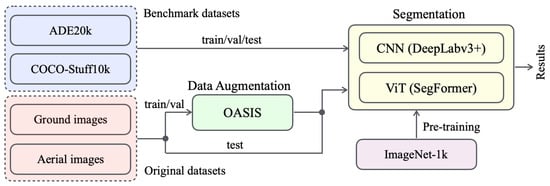
Figure 2.
Overall architecture of OutcropHyBNet.
The OutcropHyBNet architecture is designed to harness the power of CNN and ViT backbones for accurate semantic segmentation of outcrop images. The input images are processed through both backbones, allowing for efficient feature extraction and comprehensive contextual understanding. The extracted features are further processed by additional layers to perform pixel-wise classification, resulting in the generation of high-quality segmentation maps. As the baseline model for OutcropHyBNet, we integrate DeepLabv3+ and SegFormer into the architecture. Herein, SegFormer is one of the state-of-the-art semantic segmentation models that adopts a transformer-based architecture [30]. By leveraging the capabilities of SegFormer, we aim to improve the accuracy and performance of outcrop image segmentation in our proposed method. By contrast, DeepLabv3+ is a lightweight model that exhibits superiority in stuff classification. Although the ViT has gained significant attention in the field of computer vision, CNNs still demonstrate strong potential in segmentation tasks, particularly in areas involving texture and stuff [31]. For this mechanism, OutcropHyBNet can flexibly utilize both backbones based on the segmentation target.
3.1. Semantic Image Synthesis
3.1.1. Data Augmentation with GANs
Generative Adversarial Networks (GANs) [32] are a generative model based on adversarial training without extensively annotated training data [33]. GANs offer a technique for generating realistic data, such as images, from random noise. In our previous study [34], we demonstrated the power and effectiveness of image synthesis for semantic segmentation applications in agriculture.
The network architecture of GANs consists of two main components: a generator G and a discriminator D. The G is responsible for generating synthetic images, while the role of D is to distinguish between real images from a dataset and fake images generated by G. The G aims to deceive D by generating images that closely resemble real ones, while D strives to accurately classify the input images as real or fake. Both G and D networks are trained adversarially and simultaneously. The training process involves iteratively updating the networks in an attempt to achieve a dynamic equilibrium, where G becomes increasingly proficient at generating realistic images, and D becomes increasingly adept at discriminating between real and fake images. The G receives random noise as input and transforms it into synthesized images. The D, on the other hand, receives either real images from a dataset or generated images from G as input and outputs a probability score indicating the likelihood of the input being real.
By optimizing the respective objectives of G and D through backpropagation and gradient descent, GANs learn to generate high-quality synthetic data that closely resembles the real data distribution. Since their introduction, GANs have undergone significant improvements and spawned various derivative models. These improvements have expanded the capabilities of GANs and paved the way for extensive research in the realm of semantic image synthesis. In this study, we introduce OASIS [29], a novel generative model based on GANs, which harnesses the power of the adversarial training paradigm to synthesize images with desired semantic content.
3.1.2. OASIS
In recent years, research on data generation has gained significant momentum, driven by the introduction of diffusion models (DMs) [35]. Although DMs have demonstrated their efficacy in various vision tasks [36], they often require substantial computational resources and impose a heavy memory burden. In this study, prioritizing ease of implementation and computational efficiency, we have selected OASIS [29] as our model of choice, which is based on the GAN framework.
To generate high-quality images that align with the input semantic label map, G requires D, which can effectively capture semantic features at various resolutions. In the OASIS framework, the role of D is structured as a multi-class segmentation task. The architecture adopted in D is an encoder-decoder network, specifically based on the U-Net [23] with skip connections. The segmentation task for D aims to predict per-pixel class labels for real images, considering the given semantic label map as the ground truth. In addition to the N semantic classes obtained from the label map, all pixels of the synthesized images are classified as an additional class. Therefore, the formulated segmentation task involves classes, and OASIS employs a cross-entropy loss with classes for training.
As the segmentation task deals with class imbalance due to varying class frequencies, there is a possibility that the performance may be hindered. To mitigate this issue, OASIS leverages pixel-level loss calculation in D. Specifically, each class is weighted inversely proportional to the frequency of occurrence at the pixel level within a batch. This weighting scheme assigns higher weights to classes with lower frequencies, aiming to alleviate the impact of class imbalance and improve accuracy for classes with low occurrence. As a result, the contribution of each class to the loss is normalized, leading to improved accuracy for classes with low occurrence. The loss of the updated D is formulated as follows:
where x represents real images, H and W represent the image height and width, is the combination of noise and label map used by G to produce synthesized images, and D maps real or synthesized images to per-pixel -class prediction probabilities. Here, denotes a unit vector in a normed vector space. The ground truth label t is a 3D tensor, where the first two dimensions correspond to spatial positions , and the third dimension encodes the class as a one-hot vector. When designing G to align with D, the loss function for G is expressed as following.
To enable multi-modal synthesis through noise sampling, G is designed to synthesize diverse outputs from input noise. Hence, a noise tensor of size is constructed to match the spatial dimensions of the label map, where N represents the number of semantic classes, and M corresponds to the number of masks. During training, the 3D noise tensor is sampled channel-wise and fed to each pixel of the image. After sampling, the noise and label maps are concatenated along the channel dimension, forming a noise-label concatenation 3D tensor. This concatenation tensor serves as input to the first generation layer and spatially adaptive normalization layers of each generation block. The 3D noise has sensitivity at the channel and pixel levels, allowing for specific object-level image generation by sampling noise locally for each channel, label, or pixel during testing.
3.2. Semantic Segmentation
3.2.1. DeepLabv3+
For pixel-level image segmentation, DeepLabv3+ [27] represents a significant advancement within the renowned DeepLab model family [37]. This architecture has been specifically designed to excel in the task of precise and detailed segmentation, offering exceptional performance and accuracy. By leveraging advanced techniques and innovations, DeepLabv3+ pushes the boundaries of pixel-level image segmentation and stands as a testament to the ongoing progress within the DeepLab model family. DeepLabv3+ has garnered significant acclaim for their remarkable prowess in achieving precise and efficient semantic image segmentation. With its enhanced architecture and refined techniques, DeepLabv3+ builds upon the foundation established by its predecessors, pushing the boundaries of segmentation capabilities even further. Moreover, DeepLabv3+ has achieved outstanding performance on various benchmark datasets, surpassing previous state-of-the-art methods in terms of accuracy and computational efficiency. Its ability to capture contextual information at multiple scales and preserve fine details has made it particularly effective in tasks such as object recognition, scene understanding, and medical image analysis.
The architecture of DeepLabv3+ builds upon the strengths of its predecessors by incorporating an encoder-decoder structure along with atrous convolutions [38] and atrous spatial pyramid pooling (ASPP) modules [27]. The encoder network, usually based on pre-trained CNNs such as ResNet [39] or Xception [40], extracts high-level features from the input image while preserving spatial information. The atrous convolutions enable the network to capture multi-scale contextual information without significantly increasing the computational cost. The decoder network employs bilinear upsampling to restore the spatial resolution of the features obtained from the encoder. Additionally, skip connections from earlier layers are incorporated to ensure that fine-grained details are preserved in the final segmentation. The ASPP module further enhances the receptive field of the network by applying atrous convolutions at multiple dilation rates and capturing contextual information at different scales.
3.2.2. SegFormer
SegFormer [28] adopts a ViT-based methodology, leveraging its distinctive Mix Transformer (MiT) encoder. The MiT encoder consists of a hierarchical Transformer, overlapped patch merging, efficient self-attention, and Mix-FFN. These components collectively contribute to the effectiveness and efficiency of the SegFormer model for segmentation tasks. Unlike ViT, which can only generate feature maps at a single resolution, the hierarchical Transformer in SegFormer produces multi-level feature maps. These maps provide both high-resolution coarse features and low-resolution fine-grained details, contributing to improved segmentation accuracy.
ViT incorporates Positional Encoding (PE) to capture positional information. However, the resolution of PE is fixed. As a result, when the resolution differs between training and testing, the accuracy may deteriorate. To address this issue, a Mix-FFN is introduced, which applies a convolutional layer directly to the feed-forward network (FFN).
SegFormer adopts a lightweight decoder consisting solely of MLP layers, known as the All-MLP decoder. This avoids the computationally expensive configurations used in other methods. The hierarchical Transformer encoder in SegFormer enables this simple decoder by having a larger effective receptive field (ERF) compared to the encoder of traditional CNNs.
3.3. Cross-Entropy Loss
To train DeepLabv3+ and SegFormer, a large-scale dataset annotated with pixel-level labels is required. Typically, the network is trained in a supervised manner using a cross-entropy loss function given by:
where N is the number of pixels; C is the number of classes; represents the ground truth label for pixel i and class j; and is the predicted probability of pixel i belonging to class j.
3.4. Evaluation Criteria
In this study, we employ the Fréchet Inception Distance (FID) [41,42] as a formal evaluation criterion. By incorporating information about the underlying distributions and the representation of features, the FID metric provides a comprehensive assessment that captures the fidelity and resemblance of the generated samples to the real data. The FID metric utilizes a pre-trained Inception network [43] that has been trained on the ImageNet dataset [44]. The pre-training on ImageNet helps capture general visual features and enables transfer learning, where the learned representations are fine-tuned for specific tasks [45]. By leveraging the representation power of the Inception network, FID provides a quantitative measure of the quality and diversity of generated images compared to the real image distribution. FID calculates the distance between the feature vectors extracted from the real images and the generated images, quantitatively evaluating the similarity between the two. The FID is defined as follows:
where and m represent the means of the feature vectors extracted from the generated images and the real images, respectively. and C represent the covariance matrices of the feature vectors.
Subsequently, to assess the quality of segmentation, Intersection over Union (IoU) is employed as the evaluation metric in this study. IoU represents the degree of intersection between the predicted region and the ground truth region, and mIoU represents the average IoU across all classes. IoU is calculated using the following equation:
Herein, True Positive () corresponds to the instances where both the prediction and the class are true. False Positive () represents the instances where the prediction is false, but the class is true. False Negative () denotes the instances where the prediction is true, but the class is false.
4. Preliminary Performance Evaluation with Benchmark Datasets
4.1. Data Profiles and Setups
We evaluated the performance of the proposed method, OutcropHyBNet, in a general context using two benchmark datasets: COCO-Stuff10K [46] and ADE20K [47]. These datasets encompass diverse scenes and objects commonly encountered in everyday environments, facilitating a comprehensive evaluation of the proposed method’s performance in real-world scenarios.
The COCO-Stuff10K serves as an extensively utilized benchmark dataset for tasks related to scene understanding and segmentation. Comprising 10,000 high-resolution images, this dataset features pixel-wise annotations. The images within this dataset exhibit diverse resolutions, ranging from to pixels, while maintaining an aspect ratio of 3:4. The dataset provides comprehensive annotations for both objects and stuff categories. It includes 80 object categories, such as person, car, and dog, and 91 stuff categories, such as sky, grass, and road. The pixel-level annotations enable detailed semantic segmentation of scenes, facilitating the evaluation and development of advanced computer vision algorithms. Moreover, the dataset provides a wide array of visual scenes, encompassing a comprehensive spectrum of both indoor and outdoor environments. It serves as a standard benchmark for evaluating and contrasting the performance of semantic segmentation models.
The ADE20K dataset is a widely used dataset for semantic segmentation tasks. It comprises more than 20,000 high-resolution images, specifically 150 objects and 50 stuff categories. All images in the dataset have a fixed resolution of 512 × 512 pixels. The ADE20K dataset provides pixel-level annotations for both objects and stuff categories, enabling fine-grained semantic segmentation. It covers a diverse range of scenes, including indoor and outdoor environments, and captures various objects and stuff categories commonly encountered in everyday life. Moreover, the ADE20K dataset is designed to facilitate research and development in scene parsing and semantic understanding. It serves as a benchmark for evaluating the performance of semantic segmentation models and has been widely adopted in the computer vision community. The inclusion of this dataset allows for a comprehensive assessment of the generalization capability of the proposed method, OutcropHyBNet.
4.2. Experimental Setup
For this study, we utilized MMSegmentation [48], an open-source segmentation toolbox developed by OpenMMLab, as the designated implementation platform. MMSegmentation offers a comprehensive and versatile solution specifically tailored for semantic segmentation tasks. Its open-source nature and seamless integration with PyTorch provide us with a valuable resource for conducting our evaluation experiments. One of the key strengths of MMSegmentation lies in its wide array of segmentation models, catering to diverse requirements in the field. This rich collection of models establishes MMSegmentation as an invaluable asset for various developers. With its extensive toolkit, we can effectively address various segmentation tasks and explore different approaches, thereby enhancing the depth and breadth of our research and practical applications.
The computation for this study was carried out on a single NVIDIA RTX A6000 GPU. Renowned as a high-performance GPU, the A6000 is purpose-built to tackle professional workloads in various fields, including data science, deep learning, AI research, and content creation. Its exceptional capabilities make it an ideal choice for handling the intensive computational tasks. The A6000 has 10752 CUDA cores, 48 GB of GDDR6 memory, and a memory bandwidth of 768 GB/s. With its powerful architecture, it delivers exceptional performance for tasks such as deep learning training, real-time ray tracing, and high-resolution rendering. The parameters for each method were determined using the configuration file of the pretrained model that achieved the highest accuracy on the ADE20K dataset, which is provided by MMSegmentation [49].
4.3. Class Balancing for Uneven Data
To mitigate the challenge of class imbalance [50], we employed class balancing techniques [51] as a simple and practical approach for data adjustment and enhancement. Let x represent the number of pixels in a class and y represent the total number of pixels excluding unlabeled pixels. The weight w is calculated using the following equations:
where represents the median of z.
Table 1 provides a comprehensive overview of the calculated weights, which were determined considering the pixel occupancy ratio. The weights were assigned in such a way that they decrease as the pixel occupancy ratio increases, and conversely, they increase as the pixel occupancy ratio decreases. The approach aims to effectively mitigate the issue of class imbalance by assigning higher weights to underrepresented classes with lower pixel occupancy ratios. This strategy ensures that these classes receive greater attention during the training process, thereby addressing their significance in a more comprehensive manner. By incorporating these calculated weights, we aim to achieve a more balanced and accurate model performance, ultimately improving the overall effectiveness of our approach in handling imbalanced datasets.

Table 1.
Calculated weights based on pixel occupancy ratio for class balancing.
We evaluate the performance of the models using the Intersection over Union (IoU) metric for each class. Table 2 presents the comparison of class balancing results for both DeepLabv3+ and SegFormer models. From the results, we observe that class balancing has a significant impact on the performance of both models. SegFormer shows improvements in most classes, except for the Black class. The decrease in performance for the Black class in SegFormer can be attributed to a specific image (Image 10), where the IoU is significantly lower compared to other images. The IoU for the Black class in DeepLabv3+ remains relatively stable across all images.
Table 2.
Comparison of class balancing results for both models [%].
4.4. Data Augmentation
Our proposed approach, OutcropHyBNet, utilizes OASIS to generate images and augment the dataset. By leveraging OASIS-generated images, we expand the breadth and depth of our dataset, enabling a more comprehensive representation of geological features and variations. Integrating OASIS into our methodology addresses the challenge of limited real-world outcrop data and enriches the learning process of OutcropHyBNet. The combination of synthetic and real data enhances the model’s capacity to accurately analyze and interpret geological formations with improved precision and reliability.
Table 3 presents the parameters used for this purpose. In this experiment, a dataset with a sampling number of 256 images was utilized, and the same dataset was used for both training and testing. DeepLabv3+ and SegFormer were used as the comparative methods. A total of 3661 images were used for evaluation, which consisted of 333 images generated using OASIS and images from the dataset used in the full image experiment. The training and testing data were randomly allocated in a 9:1 ratio, resulting in 3294 images for training and 367 images for testing.
Table 3.
Parameters for OASIS.
Table 4 shows the results of class balancing. For the Black class, both methods improved accuracy in 4 out of 6 images. For the Red class, DeepLabv3+ improved accuracy in 10 out of 13 images, while SegFormer improved accuracy in 8 images. Similarly, for the Cyan class, DeepLabv3+ improved accuracy in 11 out of 13 images, and SegFormer improved accuracy in 8 images. Regarding the Yellow class, DeepLabv3+ improved accuracy in 6 out of 13 images, while SegFormer improved accuracy in 4 images. In terms of mIoU, DeepLabv3+ improved accuracy in 10 out of 13 images, and SegFormer improved accuracy in 6 images. It is worth noting that the Yellow class exhibited a decrease in accuracy in more than half of the images for both methods. This can be attributed to the initial weight of 0.3792, which is significantly lower compared to the absence of class balancing.
Table 4.
Comparison of class balancing results [%].
Table 5 demonstrates the improved mIoU scores achieved by incorporating OASIS-generated images. These images significantly enhance the accuracy of segmenting and classifying geological formations in our proposed approach. Both segmentation methods showed improved accuracy, denoted , for all classes compared to the dataset before augmentation. Particularly, they achieved an accuracy improvement of over 3% for the Cyan class. Therefore, it can be concluded that dataset augmentation using OASIS for data generation contributes to the improvement in accuracy. Furthermore, the consistent trend of CNNs backbones outperforming ViT backbones was observed throughout the evaluation.
Table 5.
Improved mIoU [%] for OASIS Evaluation.
4.5. Selection of Backbones
To verify the effectiveness of the proposed approach, a preliminary experiment was conducted for performance comparison using seven different network models with varying backbones. The backbones used for comparison were ResNet [39], HRNet [52], U-Net [23], Swin Transformer [53], MiT [28], ViT [10], and SVT [54]. Table 6 presents the specific parameter configurations for each backbone utilized in this experiment. The common parameters included a batch size of 8, a class count of 4, 4 sampling patterns (64, 128, 256, and 512 images), an input image size of 256 × 256 pixels, and a training epoch set to 50. Regarding the input data, a random sampling was performed on 13 images, allocating them to training and testing data in a 9:1 ratio.
Table 6.
Model configurations for semantic segmentation.
The left panel of Figure 3 illustrates the accuracy of CNN-based methods [37]. DeepLa-bv3+ [27] consistently demonstrated the highest accuracy among all sampling numbers. Additionally, across all methods, the highest accuracy was achieved when the sampling number was 256 images. Subsequently, the right panel of Figure 3 presents the accuracy of ViT and hybrid-based methods [28,57]. SegFormer consistently exhibited the highest accuracy across all sampling numbers. Moreover, excluding SEgmentation TRansformer (SETR) [57], SegFormer achieved the highest accuracy when the sampling number was 256 images.
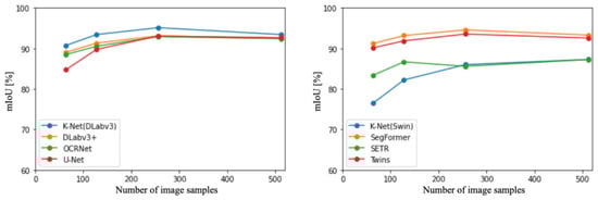
Figure 3.
Comparison of CNN-based and ViT-based methods in terms of accuracy at different sampling numbers.
Figure 4 depicts the accuracy trends and distributions for all backbones and the top two models. The red lines correspond to ViT-based backbone [10], the green lines represent hybrid backbones [57], and the blue lines represent CNN-based backbones [38]. The graph visually depicts how the accuracy of these methods varies across different experimental settings. Comparing the results, the methods can be ranked in terms of accuracy as follows: DeepLabv3+ [27], SegFormer [28], Twins [54], ResNet [39], and ViT [10]. In other words, on the original dataset, CNNs outperformed ViT in terms of accuracy for this context.
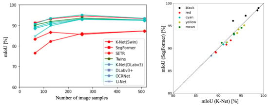
Figure 4.
Accuracy trends and distributions for all backbones and top two models.
Table 7 presents mIoU of each class [27,28]. Comparing the results, DeepLabv3+ demonstrated superiority for all classes except for the Black class at sampling numbers of 64. Additionally, in all sampling numbers except for 64 images, DeepLabv3+ outperformed SegFormer. Analyzing the mean scores, DeepLabv3+ consistently showed superior performance in all classes. Furthermore, in both methods, the classes with the highest accuracy were ranked as follows: Black, Yellow, Cyan, and Red.
Table 7.
mIoU of each class [%].
4.6. Segmentation Results
Figure 5 shows the comparison results for all classes in each dataset. In ADE20K, DeepLabv3+ achieved an mIoU of 29.36%, while SegFormer achieved an mIoU of 41.38%. SegFormer demonstrated superiority in 154 out of 171 classes (90% of the total classes). In COCO-Stuff10K, DeepLabv3+ achieved an mIoU of 38.78%, while SegFormer achieved an mIoU of 48.40%. SegFormer exhibited superiority in 138 out of 150 classes (92% of the total classes, see Appendix A).
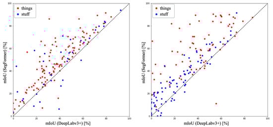
Figure 5.
Scatter plots of accuracy for DeepLabv3+ and SegFormer.
In COCO-Stuff10K, DeepLabv3+ outperformed SegFormer in terms of accuracy for certain classes. Among the things classes, DeepLabv3+ exhibited higher accuracy than SegFormer in four classes: surfboard, sports ball, car, and mouse, out of the 80 classes. In the stuff classes, DeepLabv3+ demonstrated higher accuracy in 13 classes: platform, mountain, stone, straw, bush, bridge, roof, house, cabinet, floor-other, float-wood, carpet, and wall-panel, out of the 91 classes. Conversely, SegFormer showed higher overall accuracy compared to DeepLabv3+ in both datasets. Similarly, in ADE20K, DeepLabv3+ surpassed SegFormer in accuracy for specific classes. Among the things classes, DeepLabv3+ achieved higher accuracy than SegFormer in 4 classes: railing, base, food, and monitor, out of the 115 classes. In the stuff classes, DeepLabv3+ demonstrated higher accuracy in 8 classes: house, river, skyscraper, hovel, path, tower, stairway, and pier, out of the 35 classes. Once again, SegFormer exhibited higher overall accuracy than DeepLabv3+ in ADE20K. In both datasets, the percentage of classes where DeepLabv3+ showed superiority was higher in the stuff classes compared to the things classes. This can be attributed to the fact that stuff classes lack well-defined boundaries, and the CNN-based architecture of DeepLabv3 utilized by DeepLabv3+ may have provided an advantage in texture classification, as mentioned earlier.
Table 8 presents the top score classes observed in the COCO-Stuff10K dataset, while Table 9 showcases the top score classes identified in the ADE20K dataset. These tables provide a comprehensive overview of the most prominent classes present in each dataset, shedding light on the prevalent semantic categories and objects captured in the respective datasets. The identification and analysis of these top score classes contribute to a deeper understanding of the dataset composition and can inform the development of more effective models and algorithms for semantic segmentation and scene understanding tasks.
Table 8.
Top score classes in COCO-Stuff10K [%].
Table 9.
Top score classes in ADE20K [%].
Focusing on the stuff classes, which are the classes of interest in this study, the top 10 classes combined for both methods include 3 classes (15%) in COCO-Stuff10K and 8 classes (40%) in ADE20K. On the other hand, the bottom 10 classes combined include 24 classes (75%) in COCO-Stuff10K and 9 classes (45%) in ADE20K. Therefore, it can be inferred that stuff classes have a lower representation in the top classes and a higher representation in the bottom classes.
5. Outcrop Segmentation
5.1. Custom Dataset Profile
To assess the effectiveness of the proposed method, we employed two custom benchmark datasets: stationary camera-captured ground-level images and aerial images captured by drones. The stationary images dataset consists of a collection of images captured from the perspective of a person on the ground, with meticulous attention given to their inclusion and additional insights provided by domain experts. These images were taken using a Ricoh GR III camera, an off-the-shelf device widely recognized for its high-quality imaging capabilities.
The aerial images dataset comprises images captured from drones flying at varying altitudes. These images afford a bird’s-eye view perspective, facilitating the analysis of expansive scenes and the capture of distinctive visual information. The dataset includes diverse landscapes, urban areas, and natural environments, enabling the evaluation of the proposed method’s effectiveness in aerial image analysis tasks. Both datasets were carefully curated and annotated to provide ground truth labels for evaluation. The inclusion of these custom evaluation datasets allows for a thorough assessment of the proposed method’s performance across different viewing angles and environments.
5.1.1. Stationary Ground-Level Images
Figure 6 presents the original images from our dataset, accompanied by their corresponding annotation images. The images were annotated by geological experts, who selectively cropped them to capture the regions of interest (RoI). Consequently, the image sizes exhibit variability due to the purposeful RoI extraction limited to the pertinent areas.
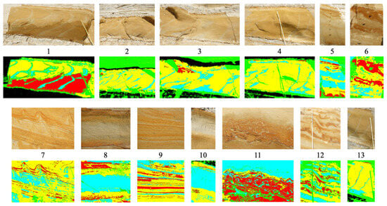
Figure 6.
Original and annotation images of our custom dataset.
Table 10 presents the relationship between geological lithology, grain size, grain sorting, and annotation colors: Yellow, Cyan, Red, and Black. Average grain size is shown on the Krumbein scale based on geological analysis. The degree of grain sorting depends on the particle size classification.
Table 10.
The relationship between geological lithology, grain size, grain sorting, and annotation colors.
Table 11 presents the resolutions in each image. Due to the burden of annotation, we clipped saliency partical images as RoIs because this is the standard way of annotation by geological experts. The burden is extremely high if the full sizes of images are set to annotation targets.
Table 11.
Image size and number.
Table 12 presents the pixel frequency for each class, providing a comprehensive overview of the distribution of pixels among different semantic classes. The presence of class imbalance within the dataset necessitates the implementation of class balancing techniques to ensure equitable representation and promote accurate model performance.
Table 12.
Pixel frequency for each class.
Our custom dataset comprises outcrop images captured using a stationary camera. These images were manually annotated by domain experts specializing in geological analysis, using four labels. For the sake of convenience, unlabeled regions were assigned None, represented by the Green label. This labeling approach facilitates the handling of regions without specific semantic attributes. The semantic classes were allocated using a color scheme, with the unlabeled pixels represented by the color green, and the labeled pixels distributed among Black, Red, Cyan, and Yellow, resulting in a total of four labels used for classification. The green pixels were excluded from the calculations, and thus the classification was performed using the remaining 4 labels across a total of 13 images, as shown in Figure 6.
5.1.2. Aerial Images
We have utilized various types of drones for sensing the vertical distributions of CO [58], horizontal distributions of particulate matter [59], and crops in rice paddy fields [60]. For this study, aerial images were obtained using the DJI Mavic 2 Pro, which is a compact drone manufactured by DJI. The process of capturing the images is depicted in Figure 7. The scale of the outcrop can be visually compared with the size of the two individuals captured in the photograph.

Figure 7.
Process of capturing aerial images with the involvement of geological experts and a drone.
Among the collected images, one specific image was chosen for evaluation, as depicted in Figure 8a. We divided this image into 64 equal-sized rectangles to make it suitable for segmentation. To facilitate the evaluation process, geological experts provided annotations for five specific labels on the image, as illustrated in Figure 8b.
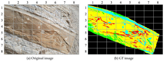
Figure 8.
Selected aerial image for evaluation.
The image used for evaluation had a resolution of pixels. The annotation data applied to this image followed the same criteria as the original dataset, performed by domain experts. The trained models used for inference were trained using the OASIS extended dataset for DeepLabv3+ and SegFormer. During inference, the aerial image was divided into an 8 × 8 grid and each sub-image was used as input. Consequently, the input size for each sub-image was pixels. The dataset consisted of a total of 64 sub-images resulting from the division.
Table 13 presents the class-wise Intersection over Union (IoU) of each image. The scores are arranged in descending order of mIoU. Although there are 13 images, there is a 2-fold difference in accuracy. Additionally, “–” indicates images that do not contain the Black label. While the individual class-wise IoU for Black is high, it represents the average value across four images. The Red class has the lowest IoU.
Table 13.
Class-wise IoU of each image [%].
Table 14 shows the correlation coefficients between the pixel occupancy ratio and ranking of each image. Note that “green” is not included as it does not affect the accuracy. The ranking of mIoU is based on the accuracy order of the average mIoU for both methods. The correlation coefficient represents the correlation between the ranking of the class’s pixel occupancy ratio and the ranking of mIoU. Negative correlation was observed for “red”. This can be attributed to the low overall pixel occupancy ratio of the Red dataset, which is 13.12%. As the pixel occupancy ratio of Red in the test data increases, the pixel occupancy ratio of Red in the training data decreases, leading to a decrease in accuracy due to insufficient data.
Table 14.
Correlation between the pixel occupancy ratio and ranking of each image [%].
Negative correlation was also observed for “Cyan”, which is believed to be for the same reasons as red. On the other hand, strong positive correlation was observed for “Yellow”. This is because the overall pixel occupancy ratio of the Yellow dataset is high at 45.22%, and the training data is sufficient. Therefore, as the pixel occupancy ratio of Yellow in the test data increases, the accuracy improves. No correlation was found for “Black”. Hence, it can be inferred that the imbalance in pixel occupancy ratio affects the accuracy. This is likely due to data insufficiency, indicating the need for techniques such as data augmentation to balance the pixel occupancy ratios.
Figure 9 illustrates the segmentation results. Table 15 presents the compared mIoU for each class. In terms of IoU, SegFormer demonstrates superiority across all classes. The overall IoU shows a difference of 8.18%. The largest accuracy difference is observed for the Black class, while the smallest difference is observed for the Yellow class.
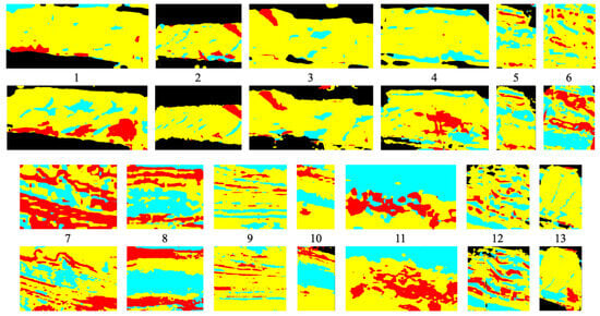
Figure 9.
Segmentation results with DeepLabv3+ (first and third rows) and SegFormer (second and fourth rows).
Table 15.
Compared mIoU for each class [%].
Confusion matrices are widely used in deep learning for evaluating the performance of classification models [61]. Due to significant variations in accuracy across images, we present the confusion matrices for image 13, which has the highest accuracy, and image 8, which has the lowest accuracy, in Figure 10, as depicted in Table 14. The Confusion Matrix reveals that the accuracy of SegFormer, compared to DeepLabv3+, is 40% higher for the Black class and 16% higher for the Cyan class. This difference in accuracy contributes to the discrepancy in mIoU.
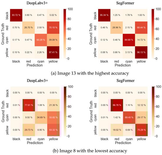
Figure 10.
Confusion matrices of the highest and lowest accuracies.
These results unequivocally demonstrate the superior performance of SegFormer in semantic segmentation compared to DeepLabv3+. The higher IoU scores obtained by SegFormer indicate its capability to better capture object boundaries and classify pixels accurately. This can be attributed to the architecture of SegFormer, which incorporates Transformer-based models, allowing for more effective feature extraction and contextual understanding. The significant accuracy difference observed for the Black class suggests that SegFormer excels in segmenting objects with complex shapes and intricate details. The Black class objects may possess fine textures or indistinct boundaries, and SegFormer’s capability to capture such nuances contributes to its superior performance. On the other hand, the minimal difference in accuracy for the Yellow class implies that both models perform similarly in segmenting objects of this class, which may have more distinguishable features or simpler shapes.
5.2. Segmentation Results of Aerial Images
In order to broaden the scope of validation and explore new possibilities, we applied OutcropHyBNet to aerial images for segmentation, expanding the range of applications in CCS. The segmentation results are evaluated using the mIoU metric, which assesses the accuracy and consistency of the predicted segmentation masks with respect to the ground truth masks. We applied our model, OutcropHyBNet, which had been trained using ground-level stationary images, to the aerial images in the dataset and obtain segmentation results. The model assigned a semantic label to each pixel, effectively distinguishing and categorizing different objects and regions within the image. The resulting segmented images provide a visual representation of the distinct entities present in the aerial scenes. By presenting the segmentation results obtained using OutcropHyBNet, we aim to demonstrate its effectiveness in segmenting aerial images.
Figure 11 presents the segmentation results obtained by applying DeepLabv3+ and SegFormer to the input image depicted in Figure 8a. The comparison reveals that SegFormer surpasses DeepLabv3+ in effectively capturing fine details and accurately delineating object boundaries. Specifically, a notable distinction can be observed in the segmentation results of the Black class, where SegFormer exhibits significantly improved performance compared to DeepLabv3+.
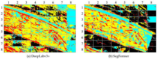
Figure 11.
Segmentation results obtained from both backbone networks for aerial images.
A comparison of the confusion matrices shown in Figure 12 reveals notable differences in accuracy between the two methods. Specifically, SegFormer achieves a 40% higher accuracy for the Black class and a 16% higher accuracy for the Cyan class compared to DeepLabv3+. These differences in accuracy directly contribute to the observed discrepancy in mean IoU (mIoU) between the two methods. The segmentation results produced by SegFormer exhibit clearer and more accurate delineation of the object classes, particularly for the Black and Cyan classes. On the other hand, DeepLabv3+ tends to produce more fragmented and less precise segmentation outputs. Overall, these figures visually demonstrate the superior performance of SegFormer in terms of accurate and detailed semantic segmentation compared to DeepLabv3+.
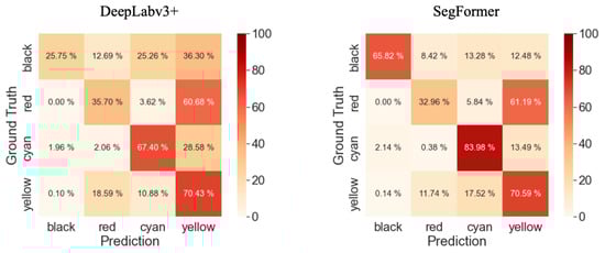
Figure 12.
Confusion matrices for both segmentation results.
Table 16 presents the average IoU for each class. It is noteworthy that SegFormer exhibits superior performance in terms of IoU for all classes when compared to DeepLabv3+. Particularly, there is a significant 40% difference in the Black class, which results in a notable 16% difference in mIoU between the two methods. Nevertheless, the mIoU scores for both methods are below 50%, highlighting the need for further improvements to enhance the segmentation accuracy for this aerial image dataset. Examining the results in Table 16, SegFormer consistently outperforms DeepLabv3+ in capturing the fine details and boundaries of the objects, leading to higher IoU scores. The Black class exhibits the largest disparity, highlighting the difficulty of accurately segmenting this class with DeepLabv3+. On the other hand, SegFormer achieves significantly better results for the Black class, indicating its effectiveness in handling such challenging scenarios. Overall, the results demonstrate that SegFormer provides improved performance in semantic segmentation tasks, especially in capturing detailed structures and enhancing the accuracy of challenging classes.
Table 16.
Comparison of mIoU for each class [%].
Figure 13 illustrates the segmentation results for the top three images based on the average mIoU scores of both backbone networks on OutcropHyBNet. These images predominantly capture the central regions of the scene. This suggests that the models have successfully captured the patterns and can generalize well to unknown images. On the other hand, the bottom images predominantly contain only the outer regions with the Black class. This indicates a potential deviation in the characteristics of the Black class compared to the original dataset. To address this issue, some of the images underwent re-annotation by experts.
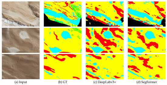
Figure 13.
Segmentation results of the top three images.
Table 17 presents the mIoU results after re-annotation. The fourth and sixth columns denote the differences in comparison to the results obtained from the initial annotation, illustrating the changes resulting from the re-annotation process. In all conditions except for SegFormer in the 1st row and 7th column, clear improvements in accuracy are observed after re-annotation. For SegFormer in the 1st row and 7th column, the model predicted the regions that turned from Cyan to Black after re-annotation as Black, resulting in a slight improvement of less than 1% in accuracy. It can be concluded that the performance improvement was limited in this case. These results suggest the potential of deep learning models to suggest re-evaluation of annotations by humans, as they can contribute to the improvement of accuracy in semantic segmentation tasks.
Table 17.
mIoU after re-annotation [%].
Figure 14 presents the segmentation results of three images from Table 17 after the re-annotation process. In comparison to the results depicted in Figure 11, the colored labels in Figure 14 have been mapped according to the texture in respective stratums.
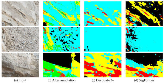
Figure 14.
Segmentation results of three images after re-annotation.
6. Conclusions
The objective of this study was to analyze the distribution of geological strata through the application of segmentation techniques on geological outcrop images, facilitating a comprehensive understanding of their spatial arrangement. We proposed OutcropHyBNet, which leverage DeepLabv3+ and SegFormer for semantic segmentation, along with OASIS for data augmentation. We conducted evaluations and comparisons of the classification performance and accuracy of both models across different classes using two publicly available benchmark datasets. In our preliminary experiments, we presented compelling evidence of the enhanced performance of DeepLabv3+ in classes heavily reliant on textures, particularly in the context of stuff classes. The superiority of DeepLabv3+ in accurately classifying textures within the dataset was observed to a significant extent, substantiating its effectiveness in such scenarios. In the evaluation experiments using our original datasets, we revealed that for non-standard objects with ambiguous shapes resembling geological strata, where classification depended on texture, CNNs exhibited superiority. Our study revealed that SegFormer outperformed other models in scenarios with limited data availability. Additionally, we identified that imbalanced class distributions had a notable impact on the accuracy of the models. Notably, we found that employing class balancing techniques resulted in enhanced accuracy for DeepLabv3+ compared to SegFormer. Moreover, our findings revealed that the utilization of OASIS for data augmentation significantly contributed to enhanced accuracy. By incorporating OASIS into the training process, we observed improved precision and performance in the classification task, highlighting the effectiveness of data augmentation techniques in enhancing the overall accuracy of the models. In the evaluation experiments conducted on ground-level images obtained using a stationary camera and aerial images obtained using a drone, we successfully demonstrated the superior performance of SegFormer across all classes. The comprehensive analysis revealed that SegFormer consistently outperformed other models in accurately classifying various objects and features present in the aerial images, highlighting its effectiveness and superiority in this specific context.
Our future endeavors encompass several challenges, including the augmentation of diversity through the collection of aerial images from various sources and types. By expanding our dataset to include a broader range of aerial images, we aim to improve the robustness and generalization capabilities of our models. Additionally, we plan to further explore and enhance data augmentation techniques to augment the diversity within the existing dataset, thereby fostering more comprehensive and representative training samples. Moreover, we will explore methods to improve the reproducibility of texture and color in image generation using GANs and DMs. We will also propose annotation modifications based on the inference results to further improve accuracy.
Author Contributions
Conceptualization, S.C.; methodology, H.M.; software, K.S. (Kodai Sato); validation, K.S. (Kodai Sato); formal analysis, K.S. (Kazuhito Sato); investigation, S.C.; resources, S.N.; data curation, T.N.; writing—original draft preparation, H.M.; writing—review and editing, H.M.; visualization, S.N.; supervision, K.S. (Kazuhito Sato); project administration, H.M.; funding acquisition, S.C. All authors have read and agreed to the published version of the manuscript.
Funding
This research received funding from the Mazda Foundation and the Japan Society for the Promotion of Science (JSPS) KAKENHI Grant Number 20K05396. More information about the grant can be found at the following links: https://mzaidan.mazda.co.jp/results/science_serach/2021.html and https://kaken.nii.ac.jp/en/grant/KAKENHI-PROJECT-20K05396/ (accessed on 1 August 2023).
Institutional Review Board Statement
Not applicable.
Informed Consent Statement
Not applicable.
Data Availability Statement
Datasets described as a result of this study are available on request to the corresponding author.
Acknowledgments
We would like to express our appreciation to Takanori Noguchi at Graduate School of International Resource Sciences, Akita University, for his great cooperation with experiments.
Conflicts of Interest
The authors declare that they have no conflict of interest. The funders had no role in the design of the study, in the collection, analyses, or in interpretation of data, in the writing of the manuscript, or in the decision to publish the results.
Abbreviations
The following abbreviations are used in this manuscript:
| ASSP | Atrous Spatial Pyramid Pooling |
| CCS | Carbon Capture and Storage |
| CNN | Convolutional Neural Network |
| CO | Carbon Dioxide |
| COCO | Common Objects in Context |
| CUDA | Compute Unified Device Architecture |
| DM | Diffusion Model |
| ERF | Effective Receptive Field |
| FCN | Fully Convolutional Networks |
| FFN | Feed-Forward Network |
| GANs | Generative Adversarial Networks |
| GPU | Graphics Processing Unit |
| IPCC | Intergovernmental Panel on Climate Change |
| IoU | Intersection over Union |
| MLP | Multi-Layer Perceptron |
| MiT | Mix Transformer |
| OASIS | Only Adversarial Supervision for Semantic Image Synthesis |
| PE | Positional Encoding |
| RoI | Regions of Interest |
| SETR | SEgmentation TRansformer |
| SGD | Stochastic Gradient Descent |
| ViT | Vision Transformer |
Appendix A
Below are the IoU scores for all classes belonging to things and stuff in the COCO-Stuff 10K and ADE20K datasets. These scores indicate the detailed accuracy of both models, DeepLabv3+ and SegFormer, in correctly segmenting the classes. The bolded numbers highlight higher scores obtained when comparing both models.
Table A1.
Class-wise IoU for things in COCO-Stuff10K [%].
Table A1.
Class-wise IoU for things in COCO-Stuff10K [%].
| Class | DeepLabv3 | SegFormer | Class | DeepLabv3 | SegFormer |
|---|---|---|---|---|---|
| tennis racket | 15.76 | surfboard | 70.94 | ||
| skateboard | 26.65 | baseball bat | 13.37 | ||
| baseball glove | 0.00 | 0.00 | kite | 45.88 | |
| sports ball | 11.14 | snowboard | 21.28 | ||
| skis | 2.78 | frisbee | 11.60 | ||
| suitcase | 25.18 | tie | 0.00 | ||
| handbag | 4.05 | umbrella | 62.33 | ||
| backpack | 5.93 | giraffe | 52.74 | ||
| zebra | 86.91 | bear | 37.99 | ||
| elephant | 59.93 | cow | 53.15 | ||
| sheep | 40.97 | horse | 71.81 | ||
| cat | 55.29 | dog | 24.11 | ||
| bird | 38.15 | bench | 29.19 | ||
| parking meter | 59.48 | traffic light | 36.82 | ||
| fire hydrant | 70.29 | stop sign | 73.00 | ||
| bicycle | 33.22 | car | 44.54 | ||
| motorcycle | 66.16 | airplane | 68.95 | ||
| bus | 70.55 | train | 60.39 | ||
| truck | 35.67 | boat | 52.48 | ||
| person | 78.55 | book | 45.09 | ||
| clock | 35.16 | vase | 46.74 | ||
| scissors | 26.62 | teddy bear | 33.03 | ||
| hair drier | 0.00 | 0.00 | toothbrush | 0.00 | |
| microwave | 34.35 | oven | 50.00 | ||
| toaster | 0.00 | sink | 42.76 | ||
| refrigerator | 50.54 | tv | 42.25 | ||
| laptop | 36.15 | mouse | 42.46 | ||
| remote | 0.84 | keyboard | 17.29 | ||
| cell phone | 24.06 | chair | 33.54 | ||
| couch | 59.02 | potted plant | 35.47 | ||
| bed | 53.02 | dining table | 48.94 | ||
| toilet | 59.77 | banana | 38.59 | ||
| apple | 1.10 | sandwich | 61.63 | ||
| orange | 25.74 | broccoli | 67.00 | ||
| carrot | 7.92 | hot dog | 41.91 | ||
| pizza | 67.11 | donut | 22.61 | ||
| cake | 17.93 | bottle | 42.24 | ||
| wine glass | 49.48 | cup | 32.78 | ||
| fork | 0.65 | knife | 3.51 | ||
| spoon | 2.49 | bowl | 42.07 |
Table A2.
Class-wise IoU for stuff in COCO-Stuff10K [%].
Table A2.
Class-wise IoU for stuff in COCO-Stuff10K [%].
| Class | DeepLabv3 | SegFormer | Class | DeepLabv3 | SegFormer |
|---|---|---|---|---|---|
| water-other | 19.24 | waterdrops | 0.00 | 0.00 | |
| sea | 65.57 | river | 11.40 | ||
| fog | 0.00 | 0.00 | ground-other | 3.14 | |
| platform | 20.55 | playingfield | 63.24 | ||
| railroad | 43.87 | road | 51.84 | ||
| pavement | 42.58 | gravel | 2.19 | ||
| mud | 0.00 | dirt | 31.02 | ||
| snow | 73.16 | sand | 50.21 | ||
| solid-other | 0.00 | 0.00 | hill | 27.78 | |
| mountain | 27.21 | stone | 0.17 | ||
| rock | 28.32 | wood | 2.88 | ||
| sky-other | 55.20 | clouds | 40.09 | ||
| plant-other | 12.16 | straw | 14.40 | ||
| moss | 0.00 | 0.00 | branch | 0.00 | |
| flower | 4.71 | bush | 15.57 | ||
| leaves | 4.00 | tree | 68.23 | ||
| grass | 68.18 | structural-other | 12.52 | ||
| railing | 8.90 | net | 28.41 | ||
| cage | 0.00 | fence | 36.62 | ||
| building-other | 51.70 | bridge | 0.62 | ||
| roof | 2.91 | tent | 38.95 | ||
| skyscraper | 9.06 | house | 28.10 | ||
| food-other | 8.13 | fruit | 9.43 | ||
| vegetable | 19.34 | salad | 0.00 | 0.00 | |
| textile-other | 2.07 | banner | 32.09 | ||
| blanket | 0.00 | 0.00 | pillow | 0.00 | 0.00 |
| cloth | 0.00 | clothes | 2.17 | ||
| curtain | 47.46 | towel | 16.01 | ||
| mat | 0.00 | rug | 38.87 | ||
| napkin | 0.00 | furniture-other | 8.68 | ||
| shelf | 5.40 | stairs | 15.86 | ||
| light | 22.23 | counter | 18.30 | ||
| cupboard | 43.17 | cabinet | 13.55 | ||
| desk-stuff | 28.84 | door-stuff | 27.93 | ||
| table | 2.51 | mirror-stuff | 25.12 | ||
| window-blind | 29.20 | window-other | 33.33 | ||
| floor-marble | 0.00 | floor-other | 21.44 | ||
| floor-stone | 0.00 | floor-tile | 33.41 | ||
| floor-wood | 46.96 | carpet | 46.40 | ||
| ceiling-other | 59.20 | ceiling-tile | 0.00 | ||
| wall-brick | 33.96 | wall-concrete | 16.80 | ||
| wall-other | 50.18 | wall-panel | 4.82 | ||
| wall-stone | 15.68 | wall-tile | 32.40 | ||
| wall-wood | 21.83 | cardboard | 0.20 | ||
| metal | 4.25 | paper | 5.53 | ||
| plastic | 0.00 |
Table A3.
Class-wise IoU for things in ADE20K [%].
Table A3.
Class-wise IoU for things in ADE20K [%].
| Class | DeepLabv3 | SegFormer | Class | DeepLabv3 | SegFormer |
|---|---|---|---|---|---|
| tree | 69.39 | bed | 84.09 | ||
| windowpane | 56.51 | cabinet | 52.60 | ||
| person | 71.29 | door | 37.36 | ||
| table | 51.40 | plant | 48.27 | ||
| curtain | 66.07 | chair | 48.92 | ||
| car | 78.68 | painting | 59.54 | ||
| sofa | 59.97 | shelf | 34.34 | ||
| mirror | 57.72 | armchair | 35.21 | ||
| seat | 51.01 | fence | 39.88 | ||
| desk | 42.37 | rock | 31.84 | ||
| wardrobe | 38.05 | lamp | 57.51 | ||
| bathtub | 60.63 | railing | 31.87 | ||
| cushion | 50.82 | base | 27.04 | ||
| box | 15.89 | column | 36.92 | ||
| signboard | 32.91 | chest of drawers | 41.70 | ||
| counter | 20.46 | sink | 62.19 | ||
| fireplace | 63.16 | refrigerator | 57.58 | ||
| stairs | 27.06 | case | 42.07 | ||
| pool table | 79.52 | pillow | 51.72 | ||
| screen door | 53.31 | bookcase | 24.73 | ||
| blind | 34.86 | coffee table | 53.47 | ||
| toilet | 77.77 | flower | 24.44 | ||
| book | 41.04 | bench | 40.14 | ||
| countertop | 52.14 | stove | 68.52 | ||
| palm | 39.55 | kitchen island | 27.19 | ||
| computer | 36.40 | swivel chair | 34.71 | ||
| boat | 25.24 | bar | 28.48 | ||
| arcade machine | 36.14 | bus | 56.52 | ||
| towel | 48.11 | light | 43.41 | ||
| truck | 25.04 | chandelier | 60.90 | ||
| awning | 13.61 | streetlight | 21.71 | ||
| booth | 22.90 | television receiver | 64.69 | ||
| airplane | 24.01 | apparel | 24.74 | ||
| pole | 17.60 | bannister | 9.32 | ||
| ottoman | 44.25 | bottle | 10.61 | ||
| buffet | 27.79 | poster | 25.29 | ||
| van | 26.74 | ship | 33.57 | ||
| fountain | 11.22 | canopy | 11.63 | ||
| washer | 51.52 | plaything | 17.54 | ||
| stool | 26.82 | barrel | 11.91 | ||
| basket | 23.40 | tent | 72.27 | ||
| bag | 4.96 | minibike | 63.70 | ||
| cradle | 72.71 | oven | 32.33 | ||
| ball | 25.58 | food | 15.93 | ||
| step | 2.08 | tank | 31.03 | ||
| trade name | 18.61 | microwave | 30.98 | ||
| pot | 35.62 | animal | 48.20 | ||
| bicycle | 47.71 | dishwasher | 59.88 | ||
| screen | 37.17 | blanket | 5.96 | ||
| sculpture | 31.79 | hood | 47.06 | ||
| sconce | 34.15 | vase | 29.11 | ||
| traffic light | 21.66 | tray | 1.21 | ||
| ashcan | 26.08 | fan | 47.26 | ||
| crt screen | 0.00 | plate | 31.14 | ||
| monitor | 7.29 | bulletin board | 22.62 | ||
| shower | 0.19 | radiator | 45.10 | ||
| glass | 8.70 | clock | 20.38 | ||
| flag | 27.18 |
Table A4.
Class-wise IoU for stuff in ADE20K [%].
Table A4.
Class-wise IoU for stuff in ADE20K [%].
| Class | DeepLabv3 | SegFormer | Class | DeepLabv3 | SegFormer |
|---|---|---|---|---|---|
| wall | 70.78 | building | 77.96 | ||
| sky | 92.35 | floor | 73.83 | ||
| ceiling | 78.69 | road | 79.11 | ||
| grass | 65.56 | sidewalk | 60.75 | ||
| earth | 31.13 | mountain | 51.07 | ||
| water | 46.40 | house | 31.97 | ||
| sea | 41.07 | rug | 48.01 | ||
| field | 26.18 | sand | 25.95 | ||
| skyscraper | 49.58 | grandstand | 32.72 | ||
| path | 19.70 | runway | 58.27 | ||
| stairway | 31.64 | river | 12.57 | ||
| bridge | 49.25 | hill | 8.62 | ||
| hovel | 8.90 | tower | 6.38 | ||
| dirt track | 3.54 | land | 0.02 | ||
| escalator | 2.68 | stage | 7.84 | ||
| conveyor belt | 42.59 | swimming pool | 26.95 | ||
| waterfall | 46.91 | lake | 18.20 | ||
| pier | 26.90 |
References
- Intergovernmental Panel on Climate Change (IPCC). Climate Change 2021: Impacts, Adaptation, and Vulnerability; IPCC: Geneva, Switzerland, 2022; Available online: https://www.ipcc.ch/report/ar6/wg2/ (accessed on 10 June 2023).
- Kang, N.; Jang, C.J.; Elsner, J.B. More than unfamiliar environmental connection to super typhoon climatology. Sci. Rep. 2023, 13, 6372. [Google Scholar] [CrossRef] [PubMed]
- Bui, M.; Adjiman, C.S.; Bardow, A.; Anthony, E.J.; Boston, A.; Brown, S.; Fennell, P.S.; Fuss, S.; Galindo, A.; Hackett, L.A.; et al. Carbon capture and storage (CCS): The way forward. Energy Environ. Sci. 2018, 11, 1062. [Google Scholar] [CrossRef]
- Wang, F.; Harindintwali, J.; Yuan, Z.; Wang, M.; Wang, F.; Li, S.; Yin, Z.; Huang, L.; Fu, Y.; Li, L.; et al. Technologies and Perspectives for Achieving Carbon Neutrality. Innovation 2021, 2, 100180. [Google Scholar] [CrossRef] [PubMed]
- Shreyash, N.; Sonker, M.; Bajpai, S.; Tiwary, S.K.; Khan, M.A.; Raj, S.; Sharma, T.; Biswas, S. The Review of Carbon Capture-Storage Technologies and Developing Fuel Cells for Enhancing Utilization. Energies 2021, 14, 4978. [Google Scholar] [CrossRef]
- Noguchi, T.; Chiyonobu, S.; Arato, H.; Satou, K.; Madokoro, H.; Nagayoshi, T. Relationship between Sorting and Porosity of Sandstones in the Pleistocene Kitaura Formation at the Oibanazaki Outcrop, Akita Prefecture, Japan. In Proceedings of the Annual Meeting of the Geological Society of Japan, Tokyo, Japan, 4–11 September 2022. (In Japanese). [Google Scholar] [CrossRef]
- Minaee, S.; Boykov, Y.; Porikli, F.; Plaza, A.; Kehtarnavaz, N.; Terzopoulos, D. Image Segmentation Using Deep Learning: A Survey. IEEE Trans. Pattern Anal. Mach. Intell. 2022, 44, 3523–3542. [Google Scholar] [CrossRef] [PubMed]
- LeCun, Y.; Bengio, Y.; Hinton, G. Deep learning. Nature 2015, 521, 436–444. [Google Scholar] [CrossRef] [PubMed]
- Long, J.; Shelhamer, E.; Darrell, T. Fully convolutional networks for semantic segmentation. IEEE Trans. Pattern Anal. Mach. Intell. 2016, 39, 640–651. [Google Scholar]
- Dosovitskiy, A.; Beyer, L.; Kolesnikov, A.; Weissenborn, D.; Zhai, X.; Unterthiner, T.; Dehghani, M.; Minderer, M.; Heigold, G.; Gelly, S.; et al. An Image is Worth 16x16 Words: Transformers for Image Recognition at Scale. arXiv 2020, arXiv:2010.11929. [Google Scholar]
- Vaswani, A.; Shazeer, N.; Parmar, N.; Uszkoreit, J.; Jones, L.; Gomez, A.N.; Kaiser, Ł.; Polosukhin, I. Attention is All You Need. In Proceedings of the 31st Conference on Neural Information Processing Systems (NeurIPS), Long Beach, CA, USA, 4–9 December 2017; pp. 5998–6008. [Google Scholar]
- Kolesnikov, A.; Beyer, L.; Zhai, X.; Puigcerver, J.; Yung, J.; Gelly, S.; Houlsby, N. Big Transfer (BiT): General Visual Representation Learning. In Lecture Notes in Computer Science; Springer: Cham, Switzerland, 2020; Volume 12350. [Google Scholar]
- Geirhos, R.; Rubisch, P.; Michaelis, C.; Bethge, M.; Wichmann, F.A.; Brendel, W. ImageNet-trained CNNs are biased towards texture; increasing shape bias improves accuracy and robustness. arXiv 2018, arXiv:1811.12231. [Google Scholar]
- Tuli, S.; Dasgupta, I.; Grant, E.; Griffiths, T.L. Are Convolutional Neural Networks or Transformers more like human vision? arXiv 2021, arXiv:2105.07197. [Google Scholar]
- Tolstikhin, I.; Houlsby, N.; Kolesnikov, A.; Beyer, L.; Zhai, X.; Unterthiner, T.; Yung, J.; Steiner, A.; Keysers, D.; Uszkoreit, J.; et al. MLP-Mixer: An all-MLP Architecture for Vision. Adv. Neural Inf. Process. Syst. 2021, 34, 24261–24272. [Google Scholar]
- Richet, R.; Borgomano, J.; Adams, E.W.; Masse, J.-P.; Viseur, S. Numerical Outcrop Geology Applied to Stratigraphical Modeling of Ancient Carbonate Platforms: The Lower Cretaceous Vercors Carbonate Platform (Se France). In SEPM Concepts in Sedimentology and Paleontology; SEPM Society for Sedimentary Geology: Tulsa, OK, USA, 2011; pp. 195–210. [Google Scholar]
- Corradetti, A.; Tavani, S.; Parente, M.; Iannace, A.; Vinci, F.; Pirmez, C.; Torrieri, S.; Giorgioni, M.; Pignalosa, A.; Mazzoli, S. Distribution and arrest of vertical through-going joints in a seismicscale carbonate platform exposure (Sorrento peninsula, Italy): Insights from integrating field survey and digital outcrop model. J. Struct. Geol. 2018, 108, 121–136. [Google Scholar] [CrossRef]
- Gupta, S.K.; Shukla, D.P. 3D Reconstruction of a Landslide by Application of UAV & Structurefrom Motion. In Proceedings of the 20th AGILE conference on Geographic Information Science, Wageningen, The Netherlands, 9–12 May 2017; pp. 9–12. [Google Scholar]
- Fernández-Lozano, J.; Gutiérrez-Alonso, G. Improving archaeological prospection using localized UAVs assisted photogrammetry: An example from the Roman Gold District of the Eria River Valley (NW Spain). J. Archaeol. Sci. Rep. 2016, 5, 509–520. [Google Scholar] [CrossRef]
- Mirkes, E.; Gorban, A.; Levesley, J.; Elkington, P.; Whetton, J. Pseudo-outcrop Visualization Of Borehole Images and Core Scans. Math. Geosci. 2017, 8, 947–964. [Google Scholar] [CrossRef]
- Zhang, Y.; Ding, W.; Xu, R.; Hu, X. CATrans: Context and Affinity Transformer For Few-shot Segmentation. In Proceedings of the Thirty-First International Joint Conference on Artificial Intelligence, Main Track, Vienna, Austria, 23–29 July 2022; pp. 1658–1664. [Google Scholar]
- Malik, O.; Puasa, I.; Lai, D. Segmentation For Multi-rock Types On Digital Outcrop Photographs Using Deep Learning Techniques. Sensors 2022, 21, 8086. [Google Scholar] [CrossRef] [PubMed]
- Ronneberger, O.; Fischer, P.; Brox, T. U-Net: Convolutional Networks for Biomedical Image Segmentation. In Proceedings of the International Conference on Medical Image Computing and Computer-Assisted Intervention, Munich, Germany, 5–10 October 2015; pp. 234–241. [Google Scholar]
- Chaurasia, A.; Culurciello, E. LinkNet: Exploiting Encoder Representations for Efficient Semantic Segmentation. In Proceedings of the 2017 IEEE Visual Communications and Image Processing (VCIP), St. Petersburg, FL, USA, 10–13 December 2017; pp. 1–4. [Google Scholar]
- Vasuki, Y.; Holden, E.-J.; Kovesi, P. An Interactive Image Segmentation Method for Lithological Boundary Detection: A Rapid Mapping Tool for Geologists. Comput. Geosci. 2017, 100, 27–40. [Google Scholar] [CrossRef]
- Tapete, D. Earth Observation, Remote Sensing, and Geoscientific Ground Investigations for Archaeological and Heritage Research. Geosciences 2019, 9, 161. [Google Scholar] [CrossRef]
- Chen, L.C.; Zhu, Y.; Papandreou, G.; Schroff, F.; Adam, H. Encoder-decoder with atrous separable convolution for semantic image segmentation. In Proceedings of the European Conference on Computer Vision (ECCV), Munich, Germany, 8–14 September 2018; pp. 801–818. [Google Scholar]
- Xie, E.; Wang, W.; Yu, Z.; Anandkumar, A.; Alvarez, J.M.; Luo, P. SegFormer: Simple and Efficient Design for Semantic Segmentation with Transformers. In Proceedings of the 35th Conference on Neural Information Processing Systems (NeurIPS 2021), Online, 6–14 December 2021. [Google Scholar]
- Sushko, V.; Schönfeld, E.; Zhang, D.; Gall, J.; Schiele, B.; Khoreva, A. OASIS: Only Adversarial Supervision for Semantic Image Synthesis. Int. J. Comput. Vis. 2022, 130, 2903–2923. [Google Scholar] [CrossRef]
- Khan, S.; Naseer, M.; Hayat, M.; Zamir, S.W.; Khan, F.S.; Shah, M. Transformers in Vision: A Survey. ACM Comput. Surv. 2022, 54, 200. [Google Scholar] [CrossRef]
- Liu, Z.; Mao, H.; Wu, C.-Y.; Feichtenhofer, C.; Darrell, T.; Xie, S. A ConvNet for the 2020s. In Proceedings of the IEEE Conference on Computer Vision and Pattern Recognition (CVPR), New Orleans, LA, USA, 18–24 June 2022; pp. 11976–11986. [Google Scholar]
- Goodfellow, I.J.; Pouget-Abadie, J.; Mirza, M.; Xu, B.; Warde-Farley, D.; Ozair, S.; Courville, A.; Bengio, Y. Generative Adversarial Networks. In Proceedings of the Advances in Neural Information Processing Systems (NeurIPS), Montreal, QC, Canada, 8–13 December 2014. [Google Scholar]
- Creswell, A.; White, T.; Dumoulin, V.; Arulkumaran, K.; Sengupta, B.; Bharath, A.A. Generative Adversarial Networks: An Overview. IEEE Signal Process. Mag. 2018, 35, 53–65. [Google Scholar] [CrossRef]
- Madokoro, H.; Takahashi, K.; Yamamoto, S.; Nix, S.; Chiyonobu, S.; Saruta, K.; Saito, T.K.; Nishimura, Y.; Sato, K. Semantic Segmentation of Agricultural Images Based on Style Transfer Using Conditional and Unconditional Generative Adversarial Networks. Appl. Sci. 2022, 12, 7785. [Google Scholar] [CrossRef]
- Sohl-Dickstein, J.; Weiss, E.; Maheswaranathan, N.; Ganguli, S. Deep unsupervised learning using non-equilibrium thermodynamics. In Proceedings of the International Conference on Machine Learning (ICML), Lille, France, 7–9 July 2015; pp. 2256–2265. [Google Scholar]
- Croitoru, F.-A.; Hondru, V.; Ionescu, R.T.; Shah, M. Diffusion Models in Vision: A Survey. IEEE Trans. Pattern Anal. Mach. Intell. 2023, 45, 10850–10869. [Google Scholar] [CrossRef] [PubMed]
- Chen, L.C.; Papandreou, G.; Kokkinos, I.; Murphy, K.; Yuille, A.L. DeepLab: Semantic Image Segmentation with Deep Convolutional Nets, Atrous Convolution, and Fully Connected CRFs. IEEE Trans. Pattern Anal. Mach. Intell. 2018, 40, 834–848. [Google Scholar] [CrossRef] [PubMed]
- Chen, L.-C.; Papandreou, G.; Schroff, F.; Adam, H. Rethinking Atrous Convolution for Semantic Image Segmentation. In Proceedings of the IEEE Conference on Computer Vision and Pattern Recognition (CVPR), Honolulu, HI, USA, 21–26 July 2017. [Google Scholar]
- He, K.; Zhang, X.; Ren, S.; Sun, J. Deep Residual Learning for Image Recognition. In Proceedings of the IEEE Conference on Computer Vision and Pattern Recognition (CVPR), Las Vegas, NV, USA, 26 June–1 July 2016; pp. 770–778. [Google Scholar]
- Chollet, F. Xception: Deep Learning with Depthwise Separable Convolutions. In Proceedings of the IEEE Conference on Computer Vision and Pattern Recognition (CVPR), Honolulu, HI, USA, 21–26 July 2017; pp. 1251–1258. [Google Scholar]
- Heusel, M.; Ramsauer, H.; Unterthiner, T.; Nessler, B.; Hochreiter, S. GANs Trained by a Two Time-Scale Update Rule Converge to a Local Nash Equilibrium. In Proceedings of the Advances in Neural Information Processing Systems (NeurIPS), Long Beach, CA, USA, 4–9 December 2017. [Google Scholar]
- Fréchet, M. Sur la distance de deux lois de probabilité. Comptes Rendus l’Acad. Sci. 1957, 244, 689–692. [Google Scholar]
- Szegedy, C.; Liu, W.; Jia, Y.; Sermanet, P.; Reed, S.; Anguelov, D.; Erhan, D.; Vanhoucke, V.; Rabinovich, A. Going Deeper with Convolutions. In Proceedings of the IEEE Conference on Computer Vision and Pattern Recognition (CVPR), Boston, MA, USA, 7–12 June 2015; pp. 1–9. [Google Scholar]
- Deng, J.; Dong, W.; Socher, R.; Li, L.-J.; Li, K.; Fei-Fei, L. ImageNet: A large-scale hierarchical image database. In Proceedings of the IEEE Conference on Computer Vision and Pattern Recognition (CVPR), Miami, FL, USA, 20–25 June 2009. [Google Scholar]
- Kornblith, S.; Shlens, J.; Le, Q.V. Do Better ImageNet Models Transfer Better? In Proceedings of the IEEE/CVF Conference on Computer Vision and Pattern Recognition (CVPR), Long Beach, CA, USA, 15–20 June 2019; pp. 2661–2671. [Google Scholar]
- Caesar, H.; Uijlings, J.; Ferrari, V. COCO-Stuff: Thing and Stuff Classes in Context. In Proceedings of the IEEE Conference on Computer Vision and Pattern Recognition (CVPR), Salt Lake City, UT, USA, 18–23 June 2018. [Google Scholar]
- Zhou, B.; Zhao, H.; Puig, X.; Fidler, S.; Barriuso, A.; Torralba, A. Scene parsing through ADE20K dataset. In Proceedings of the IEEE Conference on Computer Vision and Pattern Recognition (CVPR), Honolulu, HI, USA, 21–26 July 2017; pp. 633–641. [Google Scholar]
- MMSegmentation: OpenMMLab Semantic Segmentation Toolbox Based on PyTorch. GitHub Repository. Available online: https://github.com/open-mmlab/MMSegmentation (accessed on 10 June 2023).
- Zhou, B.; Zhao, H.; Puig, X.; Xiao, T.; Fidler, S.; Barriuso, A.; Torralba, A. Semantic understanding of scenes through the ADE20K dataset. Int. J. Comput. Vis. 2019, 127, 302–321. [Google Scholar] [CrossRef]
- Ghosh, K.; Bellinger, C.; Corizzo, R.; Branco, P.; Krawczyk, B.; Japkowicz, N. The class imbalance problem in deep learning. Mach. Learn. 2022. [Google Scholar] [CrossRef]
- Johnson, J.M.; Khoshgoftaar, T.M. Survey on deep learning with class imbalance. J. Big Data 2019, 6, 27. [Google Scholar] [CrossRef]
- Sun, K.; Zhao, Y.; Jiang, B.; Cheng, T.; Xiao, B.; Liu, D.; Mu, Y.; Wang, X.; Liu, W.; Wang, J. High-Resolution Representations for Labeling Pixels and Regions. arXiv 2019, arXiv:1904.04514. [Google Scholar]
- Liu, Z.; Lin, Y.; Cao, Y.; Hu, H.; Wei, Y.; Zhang, Z.; Lin, S.; Guo, B. Swin Transformer: Hierarchical Vision Transformer using Shifted Windows. In Proceedings of the IEEE/CVF International Conference on Computer Vision (ICCV), Virtual, 11–17 October 2021; pp. 10012–10022. [Google Scholar]
- Chu, X.; Tian, Z.; Wang, Y.; Zhang, B.; Ren, H.; Wei, X.; Xia, H.; Shen, C. Twins: Revisiting the Design of Spatial Attention in Vision Transformers. In Proceedings of the Advances in Neural Information Processing Systems 34, Online, 6–14 December 2021. [Google Scholar]
- Yuan, Y.; Chen, X.; Wang, J. Object-Contextual Representations for Semantic Segmentation. In Proceedings of the European Conference on Computer Vision (ECCV), Glasgow, UK, 23–28 August 2020. [Google Scholar]
- Zhang, W.; Pang, J.; Chen, K.; Loy, C.C. K-Net: Towards Unified Image Segmentation. In Proceedings of the Advances in Neural Information Processing Systems (NeurIPS), Online, 6–14 December 2021. [Google Scholar]
- Zheng, S.; Lu, J.; Zhao, H.; Zhu, X.; Luo, Z.; Wang, Y.; Fu, Y.; Feng, J.; Xiang, T.; Torr, P.H.S.; et al. Rethinking Semantic Segmentation From a Sequence-to-Sequence Perspective with Transformers. In Proceedings of the IEEE Conference on Computer Vision and Pattern Recognition (CVPR), Nashville, TN, USA, 20–25 June 2021; pp. 6881–6890. [Google Scholar]
- Chiba, T.; Haga, Y.; Inoue, M.; Kiguchi, O.; Nagayoshi, T.; Madokoro, H.; Morino, I. Measuring Regional Atmospheric CO2 Concentrations in the Lower Troposphere with a Non-Dispersive Infrared Analyzer Mounted on a UAV, Ogata Village, Akita, Japan. Atmosphere 2019, 10, 487. [Google Scholar] [CrossRef]
- Madokoro, H.; Kiguchi, O.; Nagayoshi, T.; Chiba, T.; Inoue, M.; Chiyonobu, S.; Nix, S.; Woo, H.; Sato, K. Development of Drone-Mounted Multiple Sensing System with Advanced Mobility for In Situ Atmospheric Measurement: A Case Study Focusing on PM2.5 Local Distribution. Sensors 2021, 21, 4881. [Google Scholar] [CrossRef]
- Madokoro, H.; Yamamoto, S.; Watanabe, K.; Nishiguchi, M.; Nix, S.; Woo, H.; Sato, K. Prototype Development of Cross-Shaped Microphone Array System for Drone Localization Based on Delay-and-Sum Beamforming in GNSS-Denied Areas. Drones 2021, 5, 123. [Google Scholar] [CrossRef]
- Marques, H.; Ferreira, J.F.; Martins, R. Confusion Matrices in Machine Learning. In Handbook of Research on Machine Learning Applications and Trends: Algorithms, Methods, and Techniques; Khoshgoftaar, M.M., Brodley, L.S., Li, C.A., Eds.; IGI Global: Hershey, PA, USA, 2020; pp. 422–443. [Google Scholar]
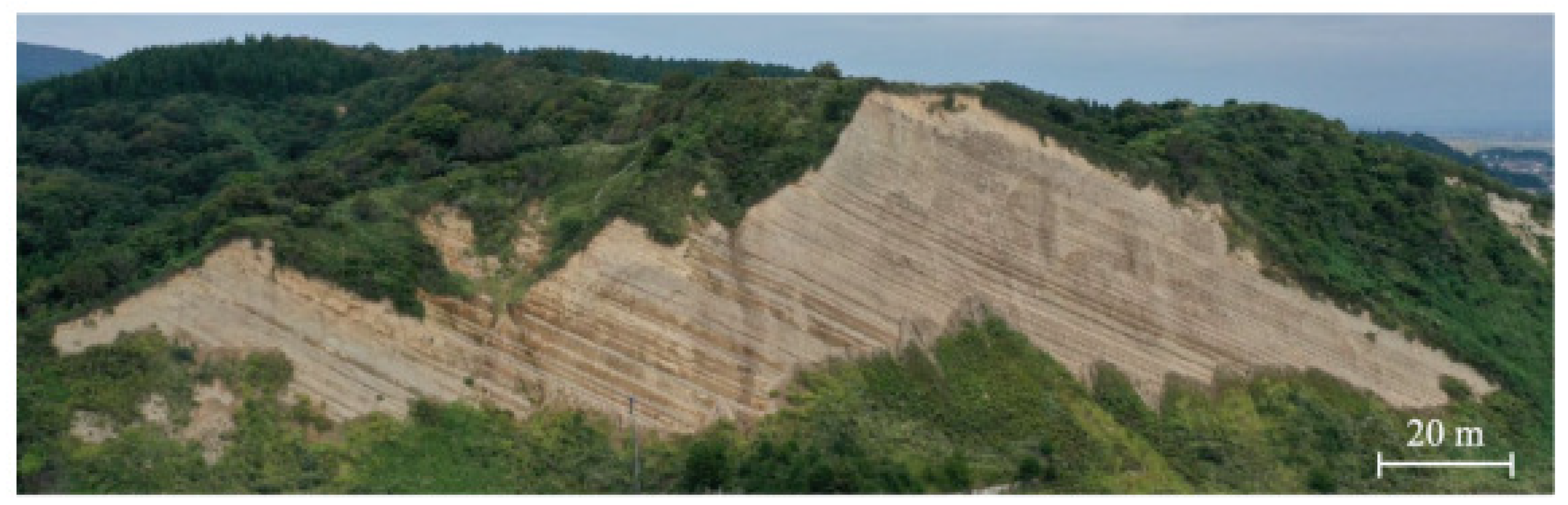
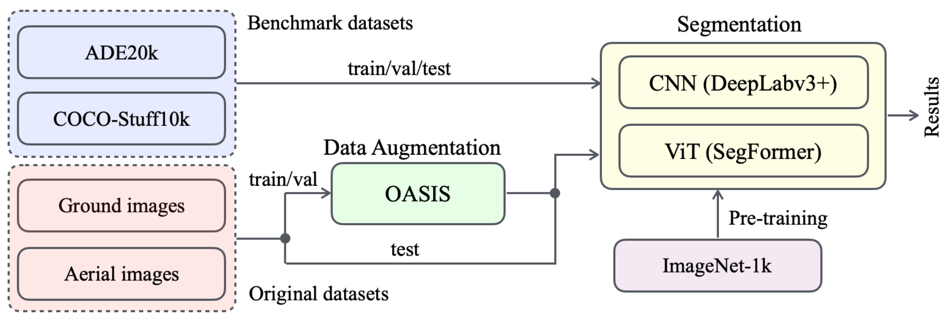
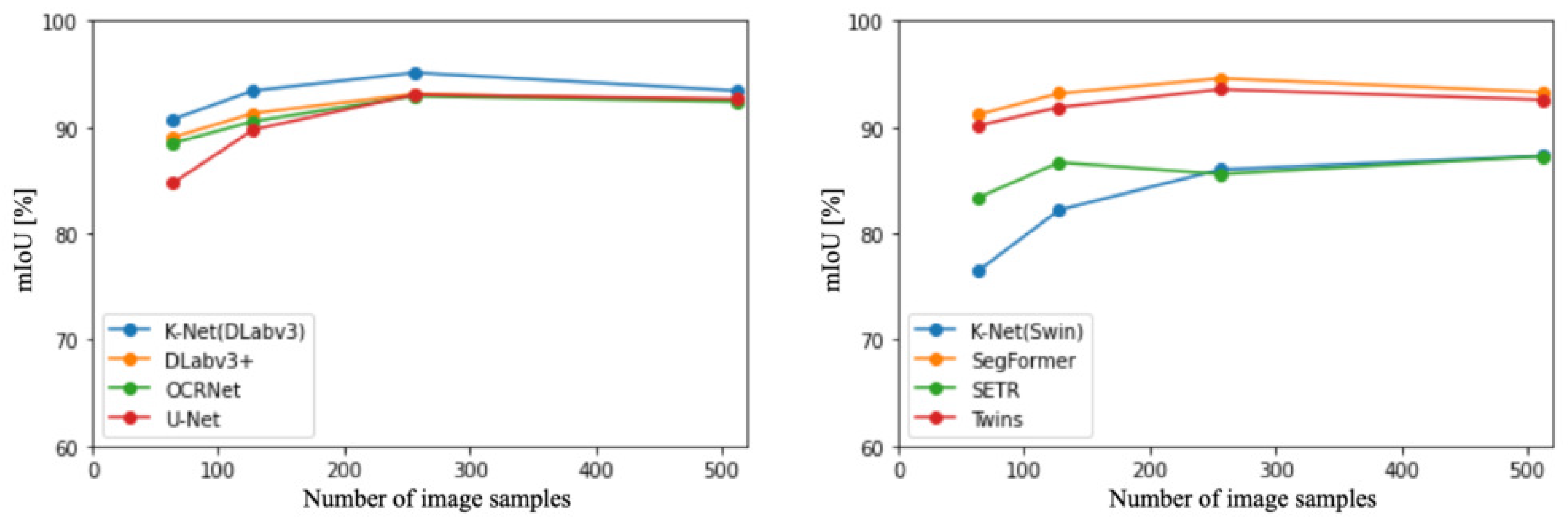
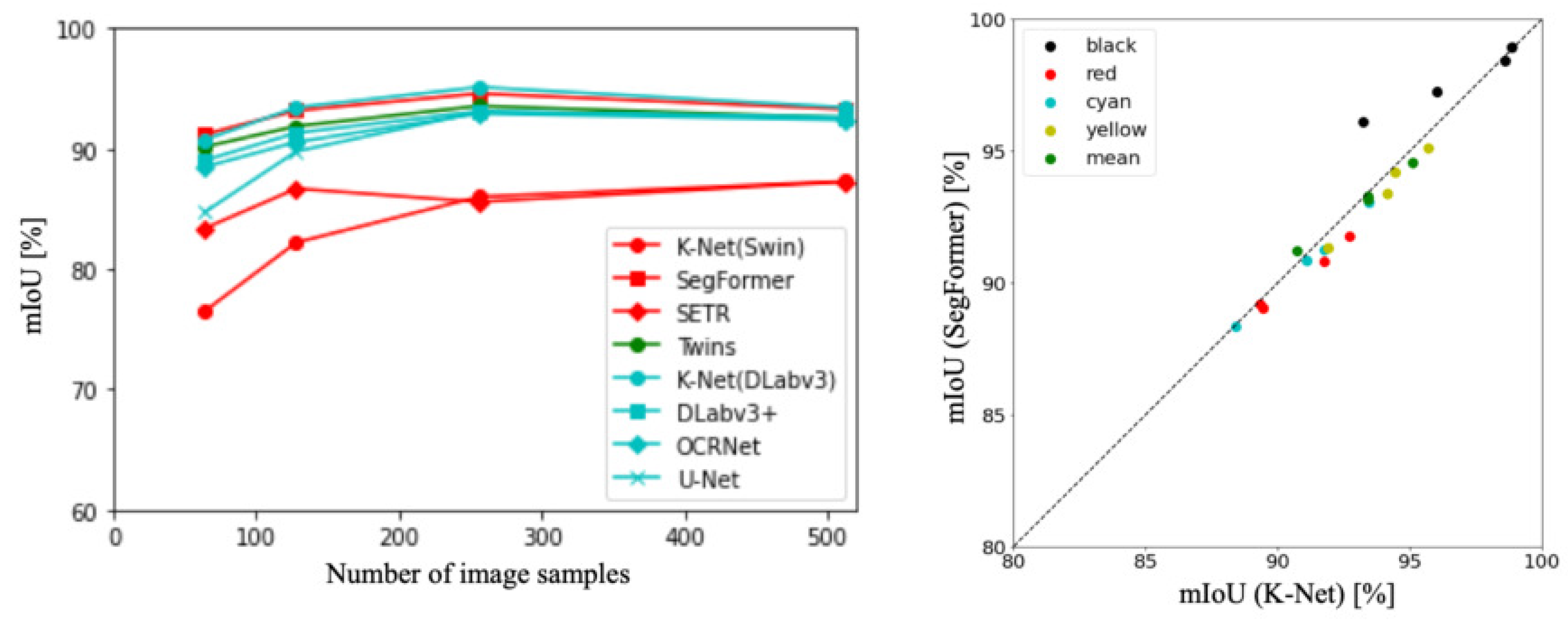
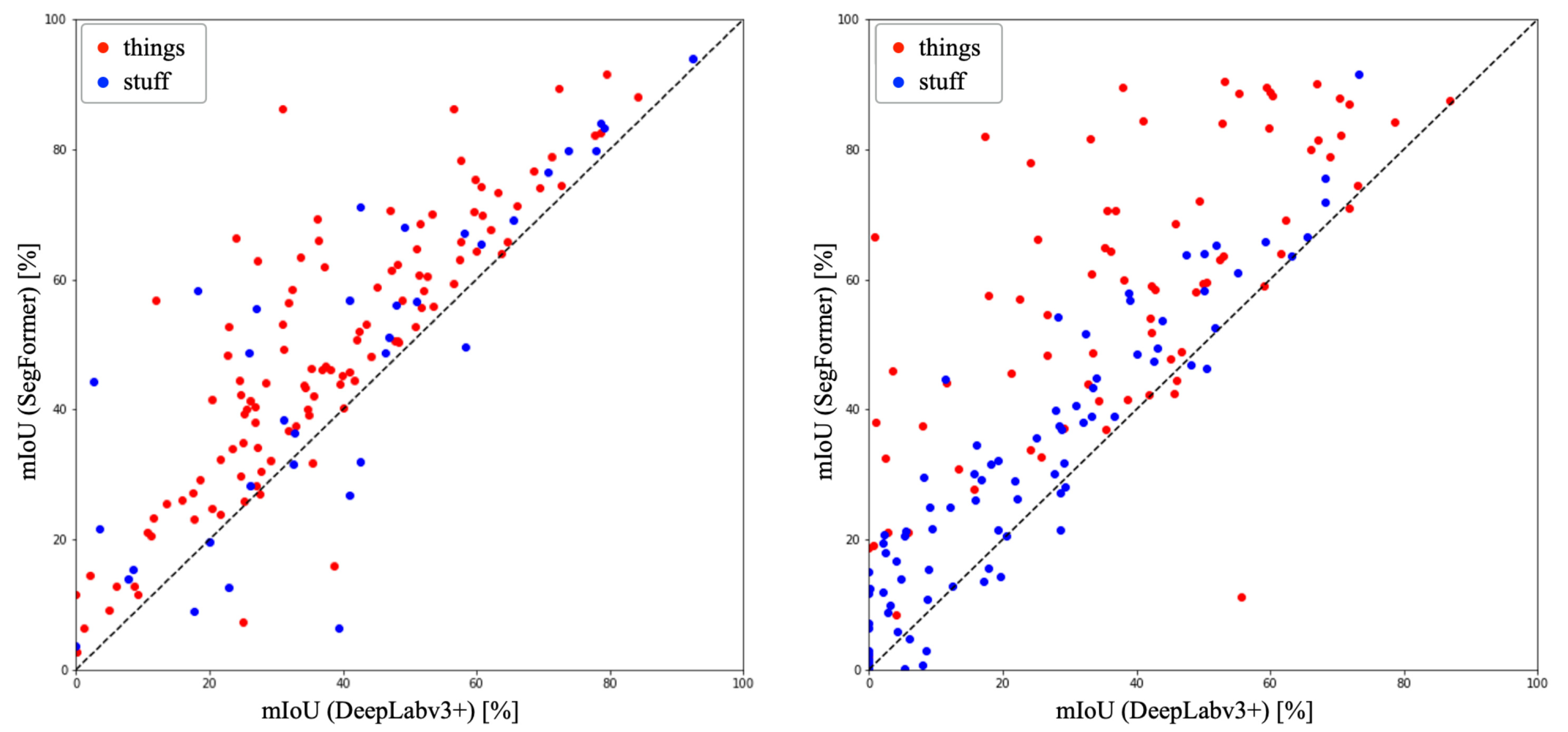
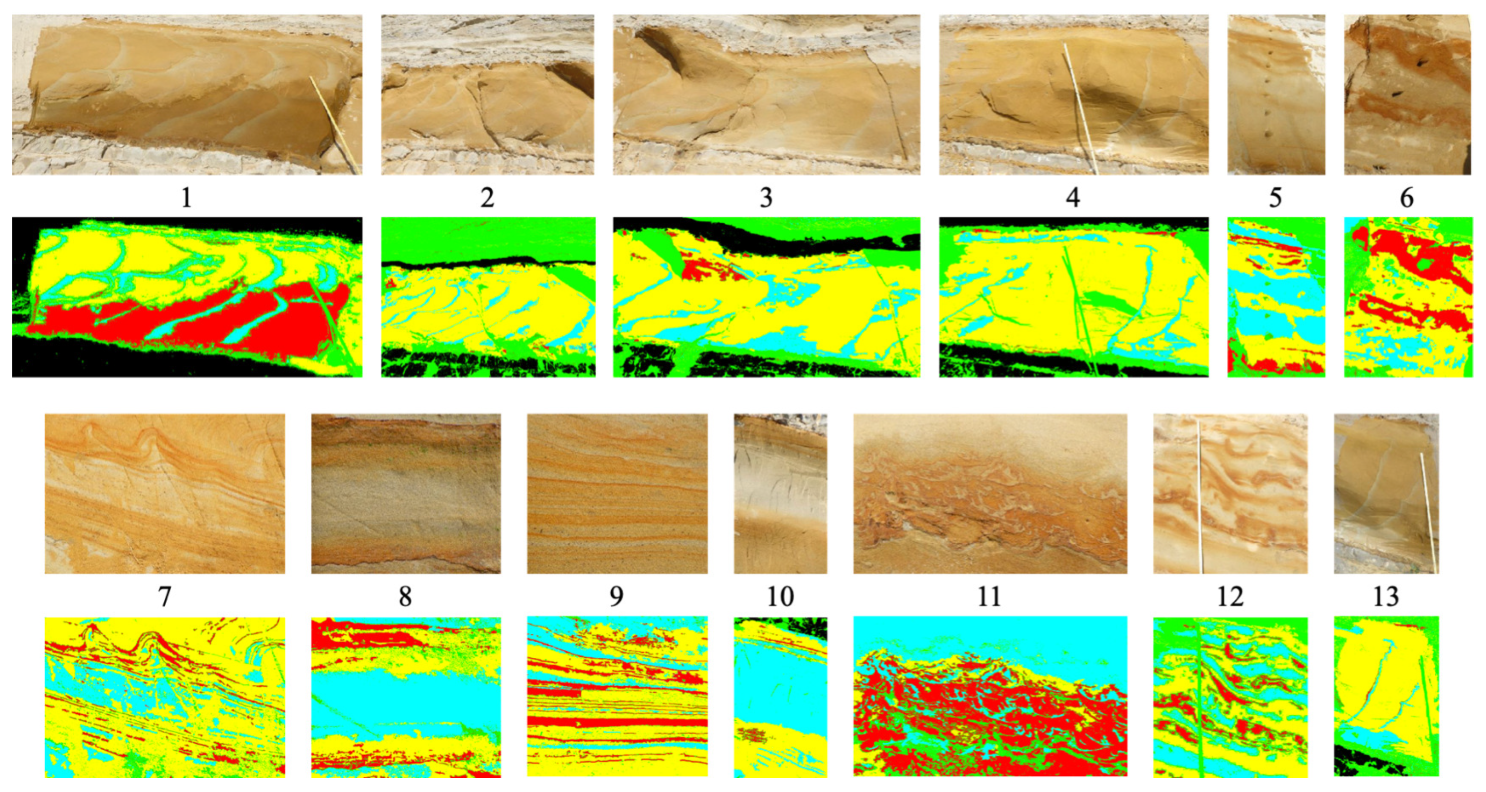
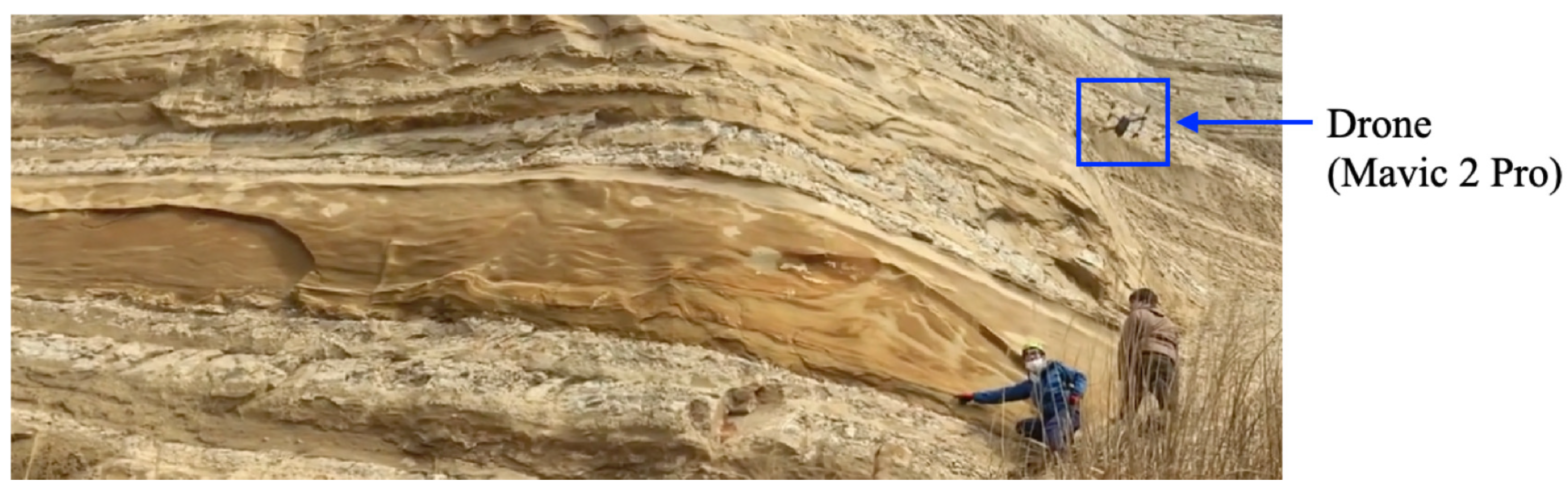

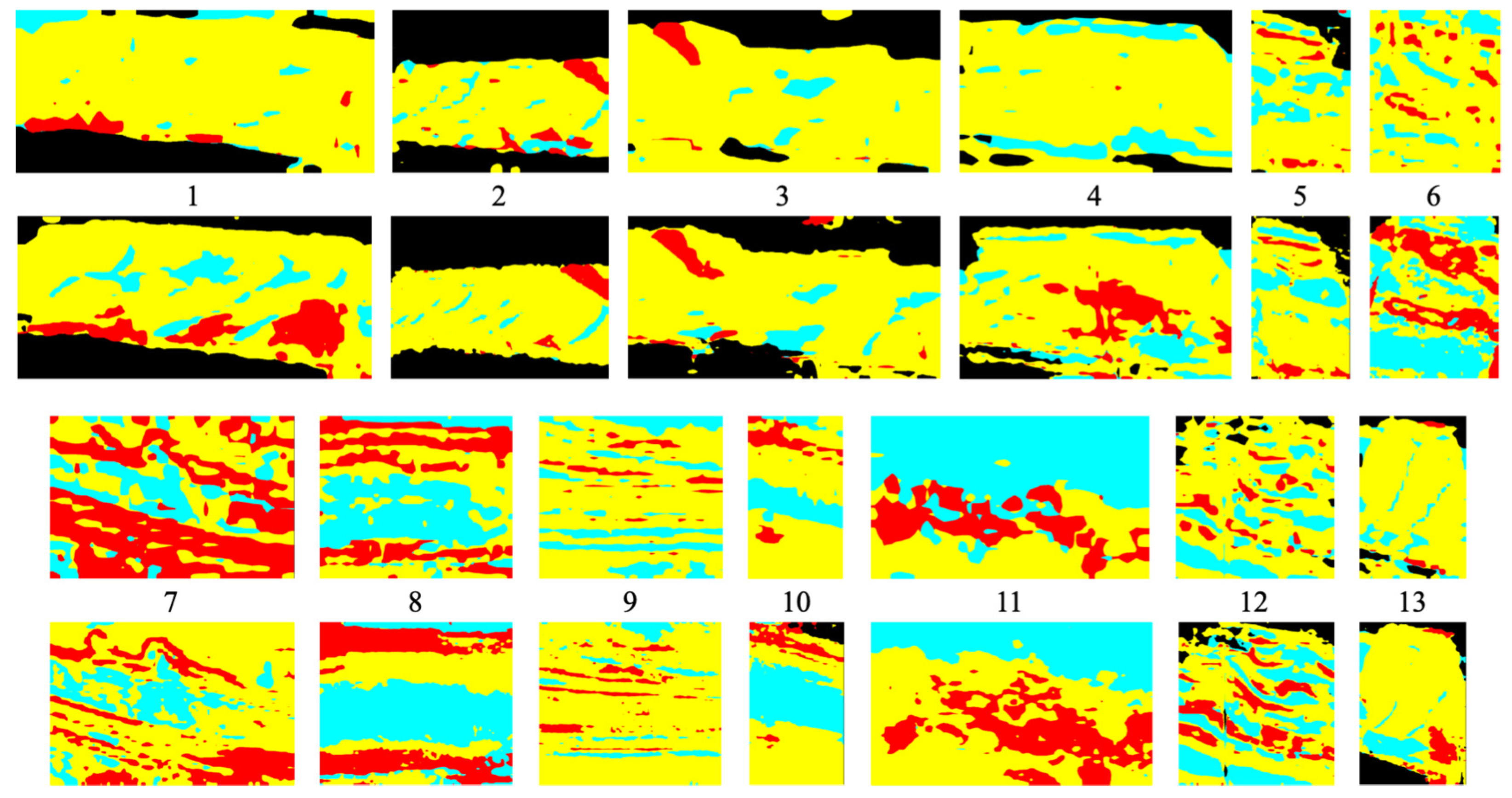


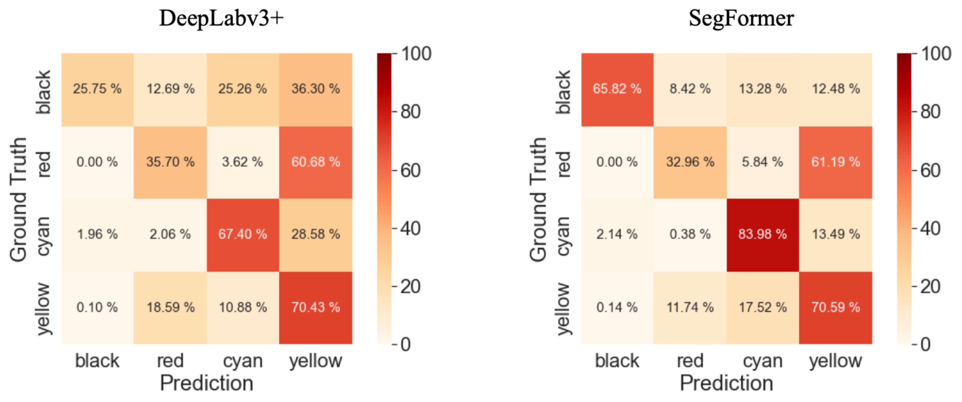
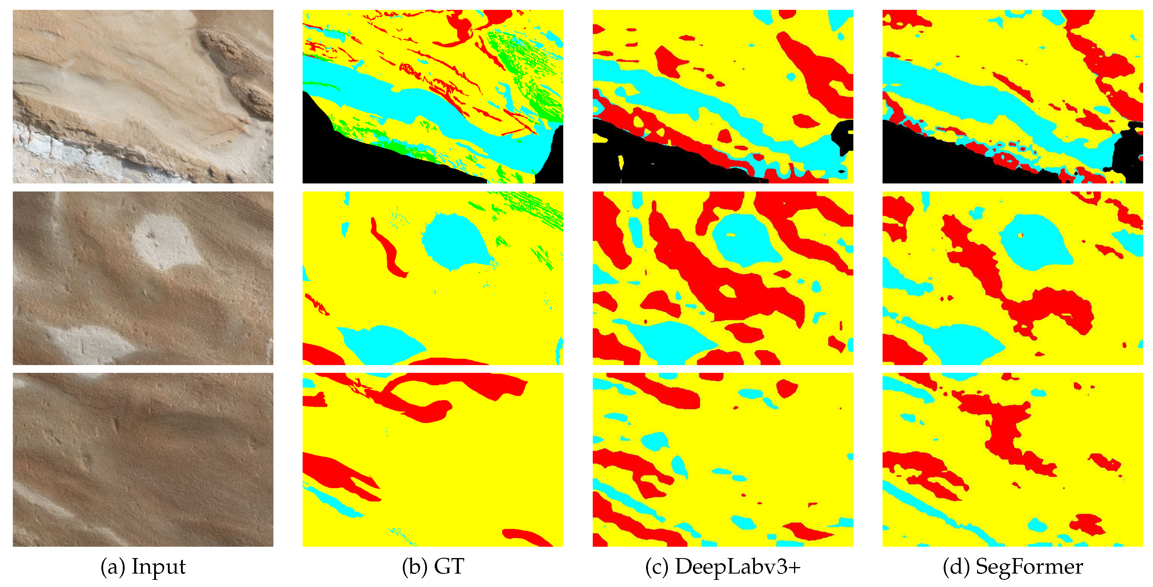

Disclaimer/Publisher’s Note: The statements, opinions and data contained in all publications are solely those of the individual author(s) and contributor(s) and not of MDPI and/or the editor(s). MDPI and/or the editor(s) disclaim responsibility for any injury to people or property resulting from any ideas, methods, instructions or products referred to in the content. |
© 2023 by the authors. Licensee MDPI, Basel, Switzerland. This article is an open access article distributed under the terms and conditions of the Creative Commons Attribution (CC BY) license (https://creativecommons.org/licenses/by/4.0/).