
A Multi-Agent Prediction Method for Data Sampling and Transmission Reduction in Internet of Things Sensor Networks


Abstract
:1. Introduction
2. Motivation and Objectives of Research
- The prediction has to be made for multiple steps ahead.
- The intervals of possible values need to be predicted.
- The high coverage of prediction intervals is required.
- The width of prediction intervals should be minimized.
3. Related Works
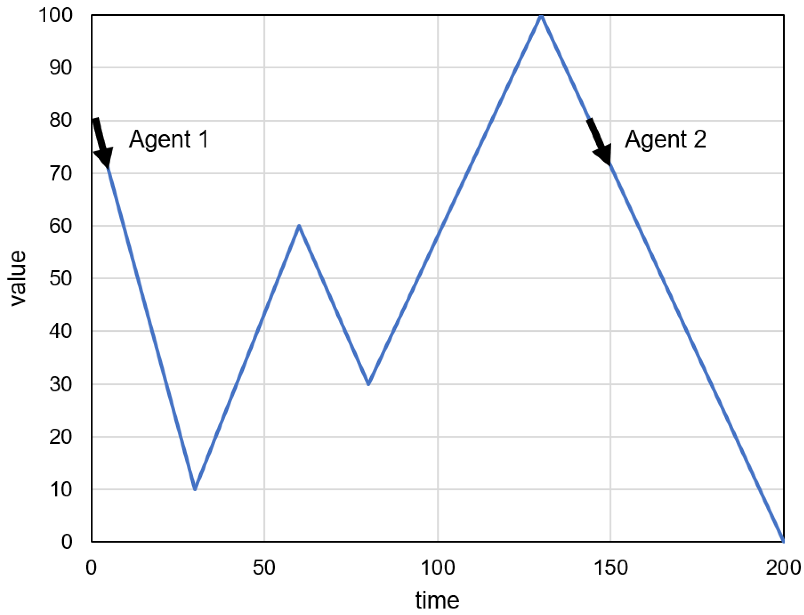
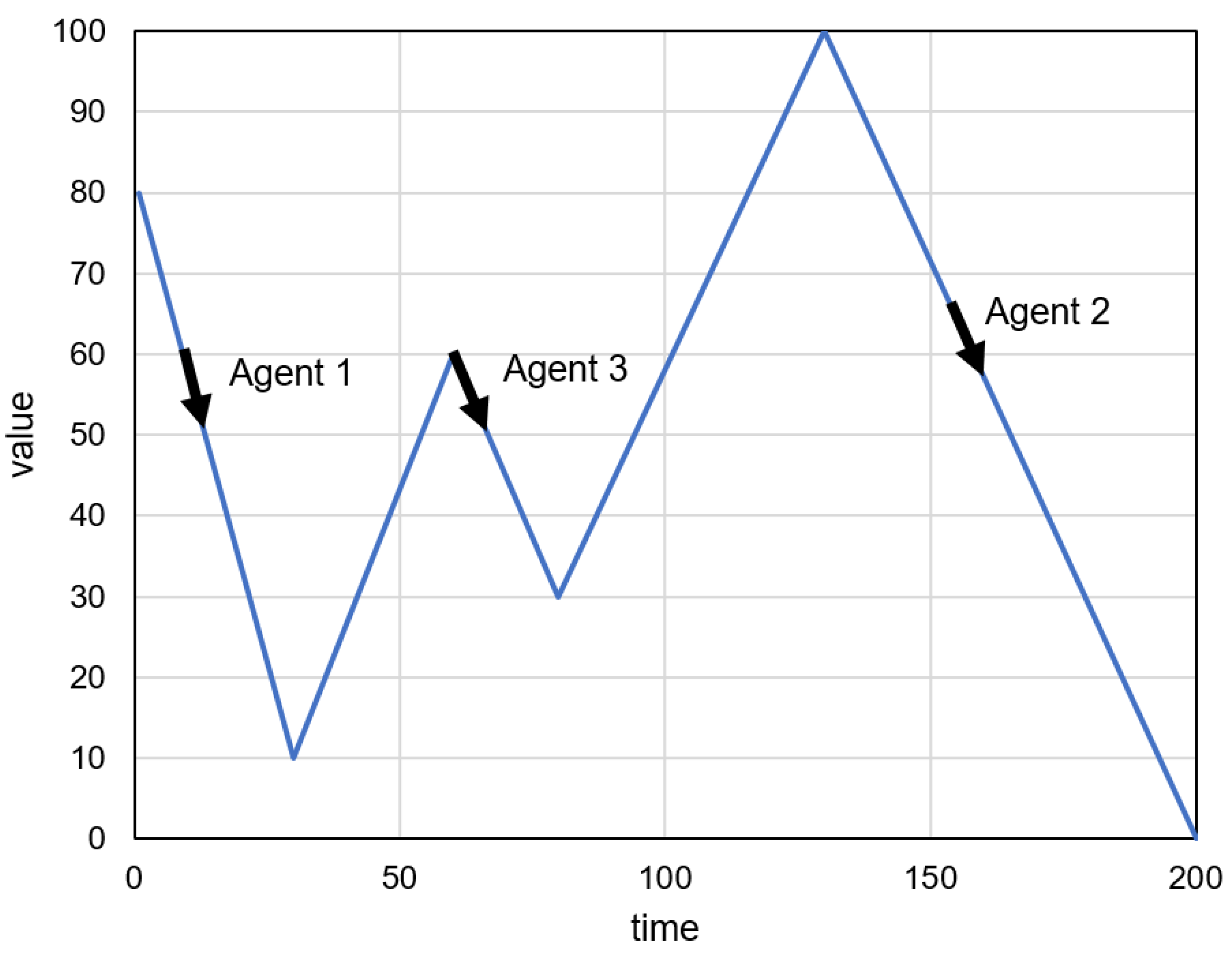
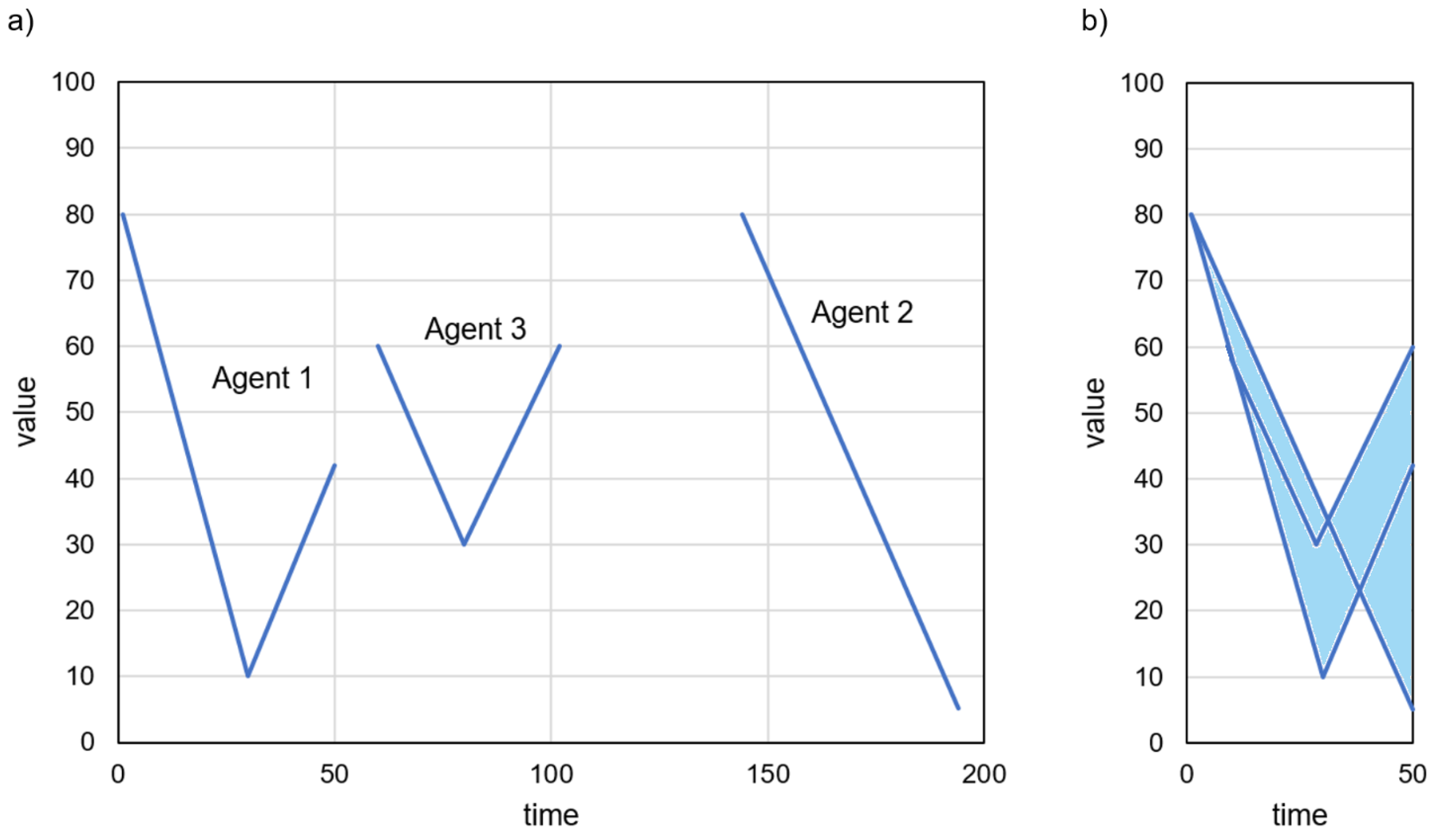
4. Proposed Method
| Algorithm 1 Multi-agent prediction |
|
| Algorithm 2 Create agents |
|
| Algorithm 3 Reproduce |
|
5. Experiments and Discussion
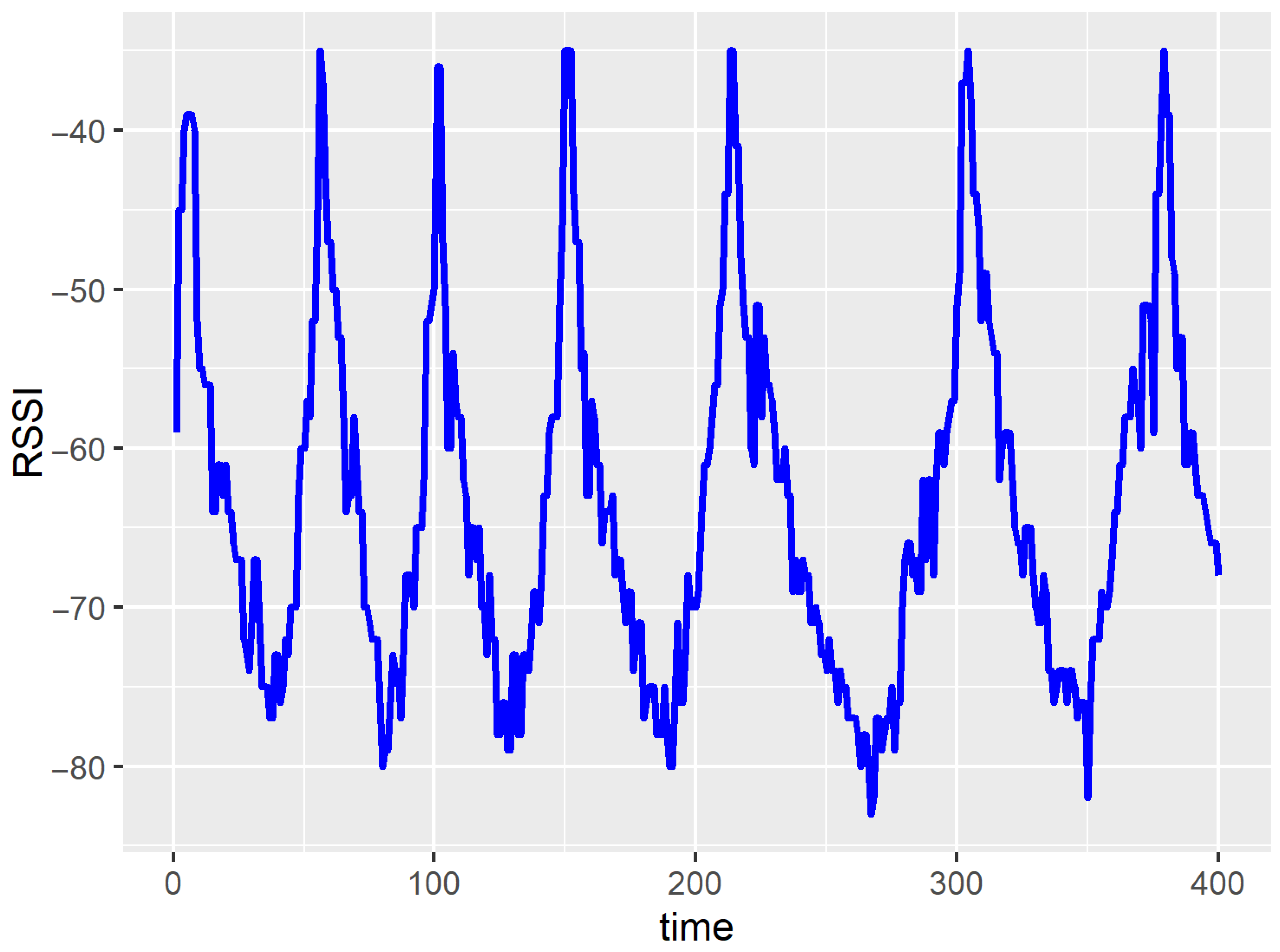
5.1. Dataset and Evaluation Criteria
5.2. Compared Methods
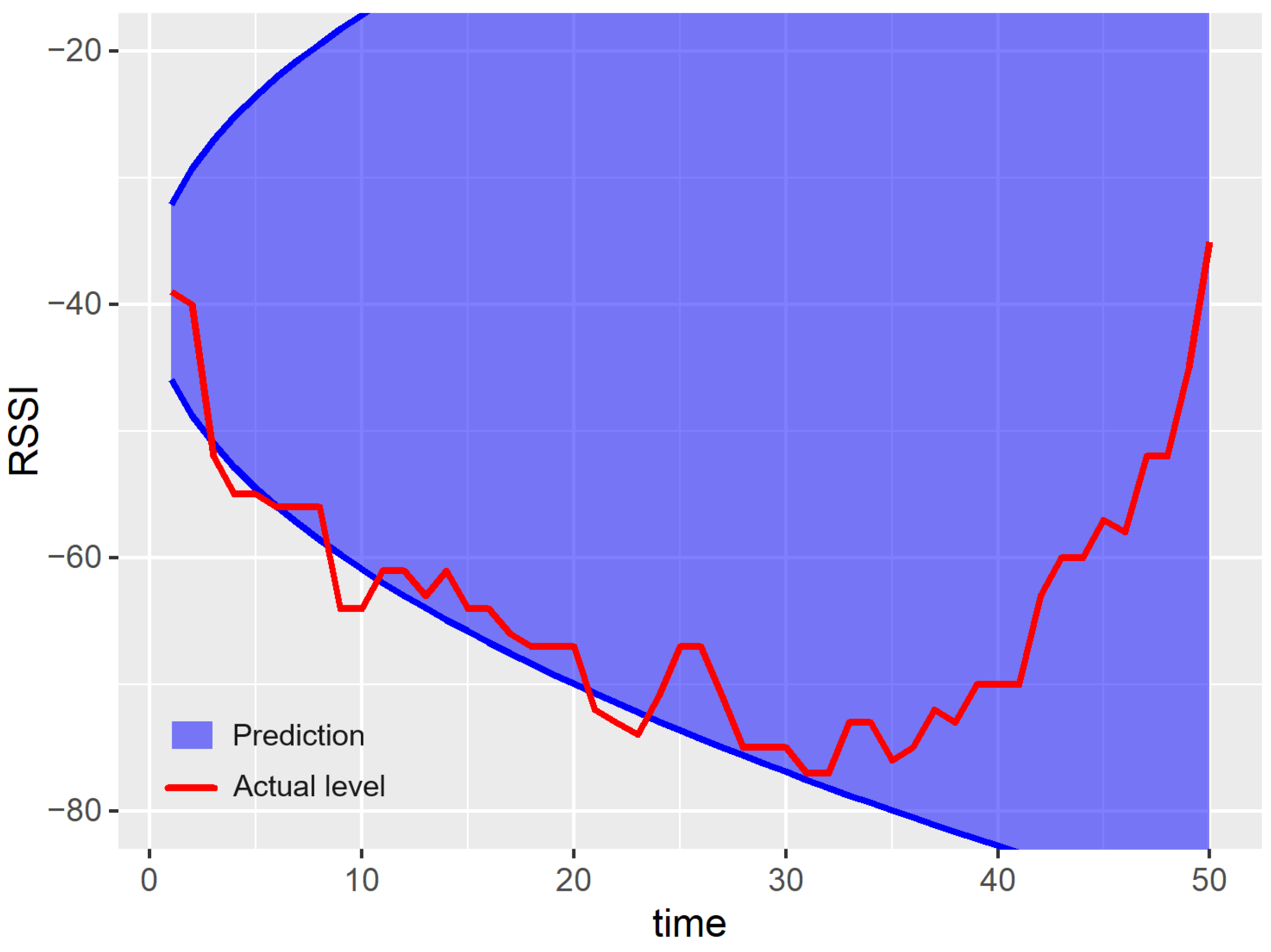
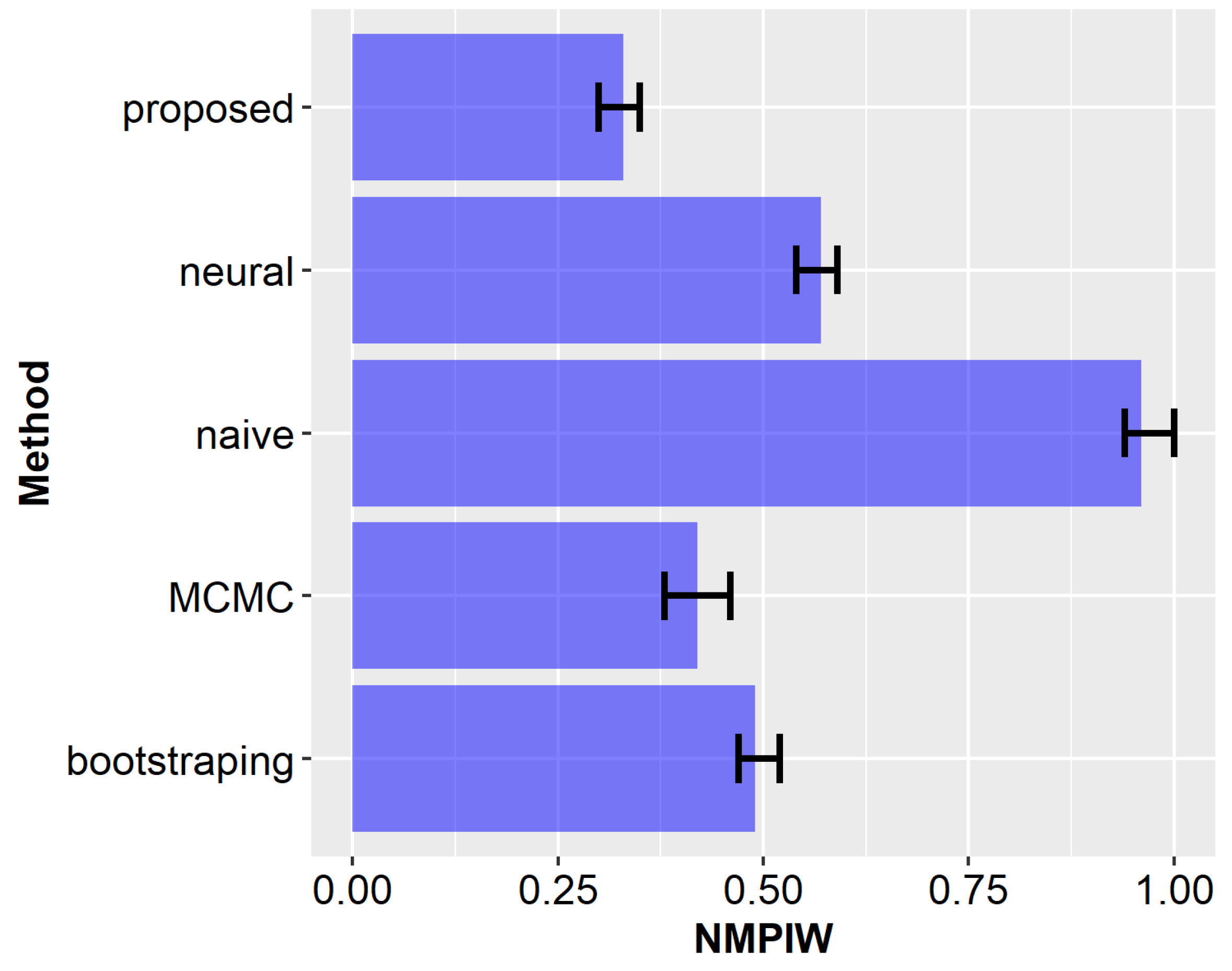
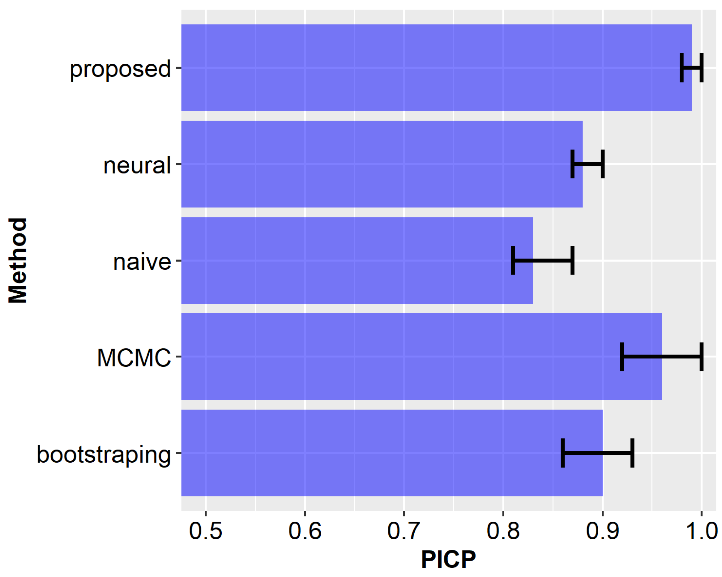
5.3. Experimental Results
6. Conclusions
Funding
Institutional Review Board Statement
Informed Consent Statement
Data Availability Statement
Conflicts of Interest
References
- Cui, Y.; Liu, F.; Jing, X.; Mu, J. Integrating sensing and communications for ubiquitous IoT: Applications, trends, and challenges. IEEE Netw. 2021, 35, 158–167. [Google Scholar] [CrossRef]
- Khanna, A.; Kaur, S. Internet of things (IoT), applications and challenges: A comprehensive review. Wirel. Pers. Commun. 2020, 114, 1687–1762. [Google Scholar] [CrossRef]
- Gulati, K.; Boddu, R.S.K.; Kapila, D.; Bangare, S.L.; Chandnani, N.; Saravanan, G. A review paper on wireless sensor network techniques in Internet of Things (IoT). Mater. Today Proc. 2022, 51, 161–165. [Google Scholar] [CrossRef]
- Sharma, S.; Verma, V.K. An integrated exploration on internet of things and wireless sensor networks. Wirel. Pers. Commun. 2022, 124, 2735–2770. [Google Scholar] [CrossRef]
- Al-Qurabat, A.K.M.; Abou Jaoude, C.; Idrees, A.K. Two tier data reduction technique for reducing data transmission in IoT sensors. In Proceedings of the 2019 15th International Wireless Communications & Mobile Computing Conference (IWCMC), Tangier, Morocco, 24–28 June 2019; IEEE: Piscataway, NJ, USA, 2019; pp. 168–173. [Google Scholar]
- Pioli, L.; Dorneles, C.F.; de Macedo, D.D.; Dantas, M.A. An overview of data reduction solutions at the edge of IoT systems: A systematic mapping of the literature. Computing 2022, 104, 1867–1889. [Google Scholar] [CrossRef]
- Lewandowski, M.; Płaczek, B. Data transmission reduction in wireless sensor network for spatial event detection. Sensors 2021, 21, 7256. [Google Scholar] [CrossRef]
- Lewandowski, M.; Płaczek, B.; Bernas, M. Classifier-based data transmission reduction in wearable sensor network for human activity monitoring. Sensors 2020, 21, 85. [Google Scholar] [CrossRef]
- Liazid, H.; Lehsaini, M.; Liazid, A. Data transmission reduction using prediction and aggregation techniques in IoT-based wireless sensor networks. J. Netw. Comput. Appl. 2023, 211, 103556. [Google Scholar] [CrossRef]
- Nedham, W.B.; Al-Qurabat, A.K.M. A review of current prediction techniques for extending the lifetime of wireless sensor networks. Int. J. Comput. Appl. Technol. 2023, 71, 352–362. [Google Scholar] [CrossRef]
- Dias, G.M.; Bellalta, B.; Oechsner, S. A survey about prediction-based data reduction in wireless sensor networks. ACM Comput. Surv. (CSUR) 2016, 49, 1–35. [Google Scholar] [CrossRef]
- Płaczek, B. Selective data collection in vehicular networks for traffic control applications. Transp. Res. Part C Emerg. Technol. 2012, 23, 14–28. [Google Scholar] [CrossRef]
- Liazid, H.; Lehsaini, M.; Liazid, A. An improved adaptive dual prediction scheme for reducing data transmission in wireless sensor networks. Wirel. Netw. 2019, 25, 3545–3555. [Google Scholar] [CrossRef]
- Malik, H.; Malik, A.S.; Roy, C.K. A methodology to optimize query in wireless sensor networks using historical data. J. Ambient. Intell. Humaniz. Comput. 2011, 2, 227–238. [Google Scholar] [CrossRef]
- Tayeh, G.B.; Makhoul, A.; Perera, C.; Demerjian, J. A spatial-temporal correlation approach for data reduction in cluster-based sensor networks. IEEE Access 2019, 7, 50669–50680. [Google Scholar] [CrossRef]
- Putra, M.A.P.; Hermawan, A.P.; Kim, D.S.; Lee, J.M. Energy efficient-based sensor data prediction using deep concatenate mlp. In Proceedings of the 2021 26th IEEE International Conference on Emerging Technologies and Factory Automation (ETFA), Vasteras, Sweden, 7–10 September 2021; IEEE: Piscataway, NJ, USA, 2021; pp. 1–4. [Google Scholar]
- Putra, M.A.P.; Hermawan, A.P.; Kim, D.S.; Lee, J.M. Data Prediction-Based Energy-Efficient Architecture for Industrial IoT. IEEE Sens. J. 2023, 23, 15856–15866. [Google Scholar] [CrossRef]
- Hussein, A.M.; Idrees, A.K.; Couturier, R. Distributed energy-efficient data reduction approach based on prediction and compression to reduce data transmission in IoT networks. Int. J. Commun. Syst. 2022, 35, e5282. [Google Scholar] [CrossRef]
- Håkansson, V.W.; Venkategowda, N.K.; Kraemer, F.A.; Werner, S. Cost-aware dual prediction scheme for reducing transmissions at IoT sensor nodes. In Proceedings of the 2019 27th European Signal Processing Conference (EUSIPCO), A Coruna, Spain, NJ, USA, 2–6 September 2019; IEEE: Piscataway, NJ, USA, 2019; pp. 1–5. [Google Scholar]
- Morales, C.R.; Rangel de Sousa, F.; Brusamarello, V.; Fernandes, N.C. Evaluation of deep learning methods in a dual prediction scheme to reduce transmission data in a WSN. Sensors 2021, 21, 7375. [Google Scholar] [CrossRef]
- Almalki, F.A.; Ben Othman, S.A.; Almalki, F.; Sakli, H. EERP-DPM: Energy efficient routing protocol using dual prediction model for healthcare using IoT. J. Healthc. Eng. 2021, 2021, 9988038. [Google Scholar] [CrossRef]
- Jarwan, A.; Sabbah, A.; Ibnkahla, M. Data transmission reduction schemes in WSNs for efficient IoT systems. IEEE J. Sel. Areas Commun. 2019, 37, 1307–1324. [Google Scholar] [CrossRef]
- Wu, F.; Chen, Y.; Chen, X.; Fan, W.; Liu, Y. An adaptive dual prediction scheme based on edge intelligence. IEEE Internet Things J. 2020, 7, 9481–9493. [Google Scholar] [CrossRef]
- Wang, H.; Yemeni, Z.; Ismael, W.M.; Hawbani, A.; Alsamhi, S.H. A reliable and energy efficient dual prediction data reduction approach for WSNs based on Kalman filter. IET Commun. 2021, 15, 2285–2299. [Google Scholar] [CrossRef]
- Fathalla, A.; Li, K.; Salah, A.; Mohamed, M.F. An LSTM-based distributed scheme for data transmission reduction of IoT systems. Neurocomputing 2022, 485, 166–180. [Google Scholar] [CrossRef]
- Lu, J.; Ding, J.; Dai, X.; Chai, T. Ensemble stochastic configuration networks for estimating prediction intervals: A simultaneous robust training algorithm and its application. IEEE Trans. Neural Netw. Learn. Syst. 2020, 31, 5426–5440. [Google Scholar] [CrossRef]
- Tian, Q.; Nordman, D.J.; Meeker, W.Q. Methods to compute prediction intervals: A review and new results. Stat. Sci. 2022, 37, 580–597. [Google Scholar] [CrossRef]
- Nourani, V.; Paknezhad, N.J.; Tanaka, H. Prediction Interval Estimation Methods for Artificial Neural Network (ANN)-based modeling of the hydro-climatic processes, a review. Sustainability 2021, 13, 1633. [Google Scholar] [CrossRef]
- Hyndman, R.J.; Athanasopoulos, G. Forecasting: Principles and Practice; OTexts: Melbourne, Australia, 2018. [Google Scholar]
- Hyndman, R.; Athanasopoulos, G.; Bergmeir, C.; Caceres, G.; Chhay, L.; O’Hara-Wild, M.; Petropoulos, F.; Razbash, S.; Wang, E.; Yasmeen, F. Forecast: Forecasting Functions for Time Series and Linear Models; R package version 8.21.1.9000. Available online: https://pkg.robjhyndman.com/forecast/ (accessed on 3 July 2023).
- Kreiss, J.P.; Lahiri, S.N. Bootstrap methods for time series. In Handbook of Statistics; Elsevier: Amsterdam, The Netherlands, 2012; Volume 30, pp. 3–26. [Google Scholar]
- Petropoulos, F.; Spiliotis, E. The wisdom of the data: Getting the most out of univariate time series forecasting. Forecasting 2021, 3, 478–497. [Google Scholar] [CrossRef]
- Martínez, F.; Frías, M.P.; Charte, F.; Rivera, A.J. Time Series Forecasting with KNN in R: The tsfknn Package. R J. 2019, 11, 229. [Google Scholar] [CrossRef]
- Lee, D. A tutorial on spatio-temporal disease risk modelling in R using Markov chain Monte Carlo simulation and the CARBayesST package. Spat.-Spatio-Temporal Epidemiol. 2020, 34, 100353. [Google Scholar] [CrossRef]
- Wu, T.; Ai, X.; Lin, W.; Wen, J.; Weihua, L. Markov chain Monte Carlo method for the modeling of wind power time series. In Proceedings of the IEEE PES Innovative Smart Grid Technologies, Washington, DC, USA, 16–20 January 2012; IEEE: Piscataway, NJ, USA, 2012; pp. 1–6. [Google Scholar]
- Shamshad, A.; Bawadi, M.; Hussin, W.W.; Majid, T.A.; Sanusi, S. First and second order Markov chain models for synthetic generation of wind speed time series. Energy 2005, 30, 693–708. [Google Scholar] [CrossRef]
- R Core Team. R: A Language and Environment for Statistical Computing; R Foundation for Statistical Computing: Vienna, Austria, 2021. [Google Scholar]
- Mader, M.; Mader, W.; Sommerlade, L.; Timmer, J.; Schelter, B. Block-bootstrapping for noisy data. J. Neurosci. Methods 2013, 219, 285–291. [Google Scholar] [CrossRef]


Disclaimer/Publisher’s Note: The statements, opinions and data contained in all publications are solely those of the individual author(s) and contributor(s) and not of MDPI and/or the editor(s). MDPI and/or the editor(s) disclaim responsibility for any injury to people or property resulting from any ideas, methods, instructions or products referred to in the content. |
© 2023 by the author. Licensee MDPI, Basel, Switzerland. This article is an open access article distributed under the terms and conditions of the Creative Commons Attribution (CC BY) license (https://creativecommons.org/licenses/by/4.0/).
Share and Cite
Płaczek, B. A Multi-Agent Prediction Method for Data Sampling and Transmission Reduction in Internet of Things Sensor Networks. Sensors 2023, 23, 8478. https://doi.org/10.3390/s23208478
Płaczek B. A Multi-Agent Prediction Method for Data Sampling and Transmission Reduction in Internet of Things Sensor Networks. Sensors. 2023; 23(20):8478. https://doi.org/10.3390/s23208478
Chicago/Turabian StylePłaczek, Bartłomiej. 2023. "A Multi-Agent Prediction Method for Data Sampling and Transmission Reduction in Internet of Things Sensor Networks" Sensors 23, no. 20: 8478. https://doi.org/10.3390/s23208478
APA StylePłaczek, B. (2023). A Multi-Agent Prediction Method for Data Sampling and Transmission Reduction in Internet of Things Sensor Networks. Sensors, 23(20), 8478. https://doi.org/10.3390/s23208478