
RBF-Based Camera Model Based on a Ray Constraint to Compensate for Refraction Error


Abstract
:1. Introduction
- We introduce an RBF-based camera model designed to counteract the refraction error engendered by diverse types of transparent shields.
- Through optimizing the RBF kernel utilizing the outcomes of GPR and ray constraint, the model attains robust performance, even amidst 3D data sparsity and measurement noise present in the calibration data.
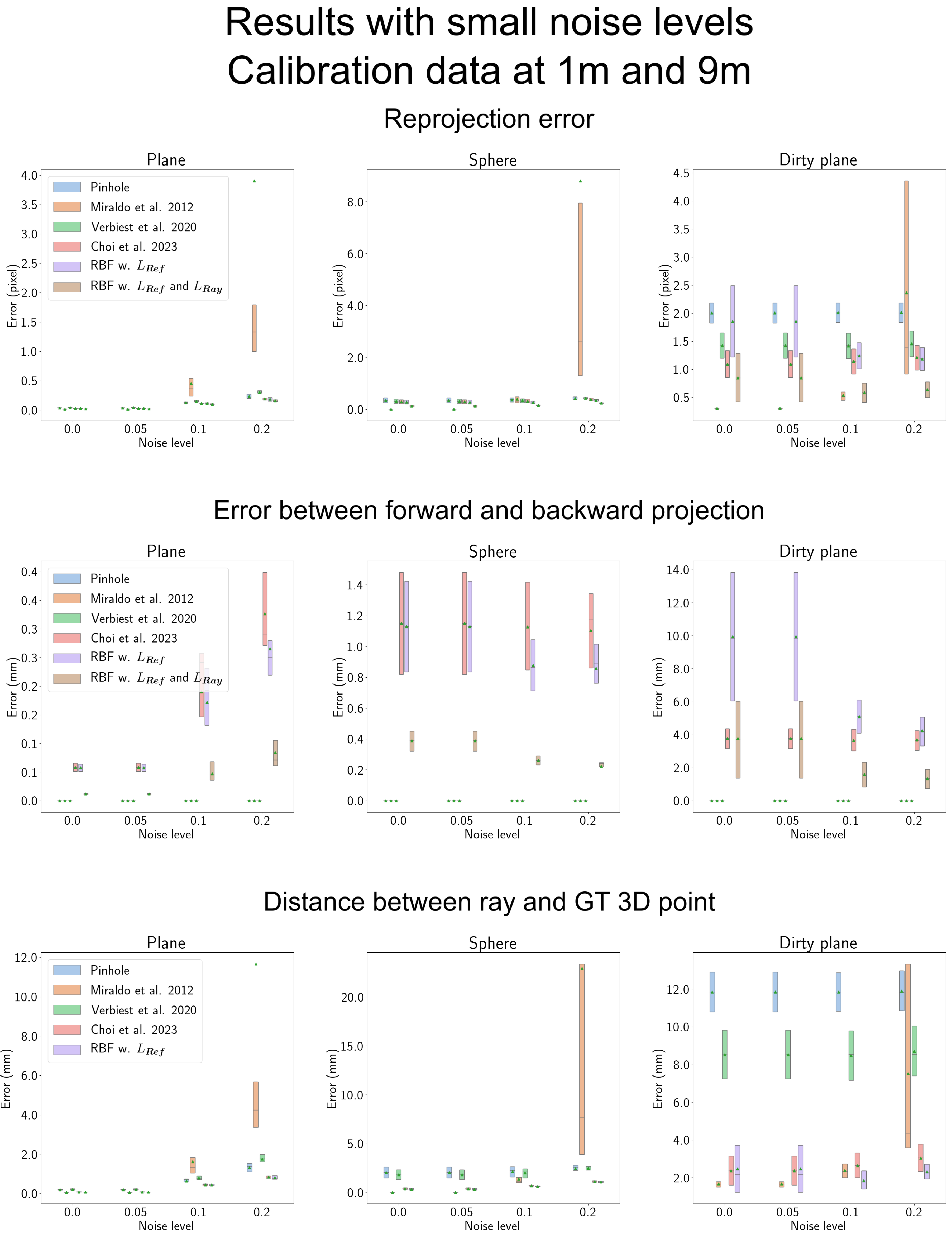
- The efficacy of the proposed method is evidenced by a reduction in the distance between the estimated ray and ground truth 3D point and a decrease in reprojection error by approximately 6% and 26%, respectively.
2. Related Work
2.1. Simple Camera Models
2.2. Camera Model Explicitly Models the Ray Path

| Method | Explanation | |
|---|---|---|
| Camera model that explicitly models the path of the camera ray | Cassidy et al. [5] | Propose a multi-view stereo system for reconstructing objects in a transparent medium. |
| Pros: Effective 3D reconstruction of objects in the transparent medium. | ||
| Cons: Requires precise information about the transparent medium. | ||
| Pavel et al. [4] | Model the surface of the transparent shield using RBF kernel. | |
| Pros: Can handle the slightly deformed surface of the transparent shield. | ||
| Cons: Requires information about the transparent shield. | ||
| Yoon et al. [6] | Propose model and the calibration method for the partially known curved-shape transparent shield. | |
| Pros: Applicable to partially known transparent shields. | ||
| Cons: Requires additional observation points inside the shield. | ||
| Generalized camera model | Grossberg et al. [8] | Firstly propose a concept of generalized camera model. |
| Pros: Applicable to any camera system. | ||
| Cons: Requires an active 2D calibration pattern. | ||
| Ramalingam et al. [10] | Propose a calibration method that relies on a minimum of three 2D calibration patterns. | |
| Pros: Requires only 2D calibration patterns. | ||
| Cons: Exhibits lower performance due to the use of 2D calibration data. | ||
| RoseBrock et al. [15,23] | Employ splines for interpolating the 2D calibration pattern. | |
| Pros: Effectively interpolates the sparse 2D calibration data. | ||
| Cons: Exhibits lower performance due to the use of 2D calibration data. | ||
| Beck et al. [12] | Use spline to model the refracted ray. | |
| Pros: Efficiently models refracted rays caused by transparent shields. | ||
| Cons: Assumes the refracted rays converge on one point, which is not valid. | ||
| Miraldo et al. [11] | Directly estimate the ray from RBF using 3D calibration data. | |
| Pros: Estimates the ray accurately under low-noise conditions. | ||
| Cons: Exhibits reduced performance as noise levels increase. | ||
| Verbiest et al. [13] | Estimate the windshield refraction using 2D residual error vectors. | |
| Pros: Effectively models the refraction in the windshield. | ||
| Cons: Uses the strong assumption that the refraction is inversely proportional to the depth. | ||
| Choi et al. [14] | Estimate the error of simple camera model using 3D error vectors. | |
| Pros: Demonstrates high performance and robustness against data noise in various types of camera systems. | ||
| Cons: Requires dense 3D calibration data and can have mismatches between forward and backward projection models. | ||
2.3. Generalized Camera Model
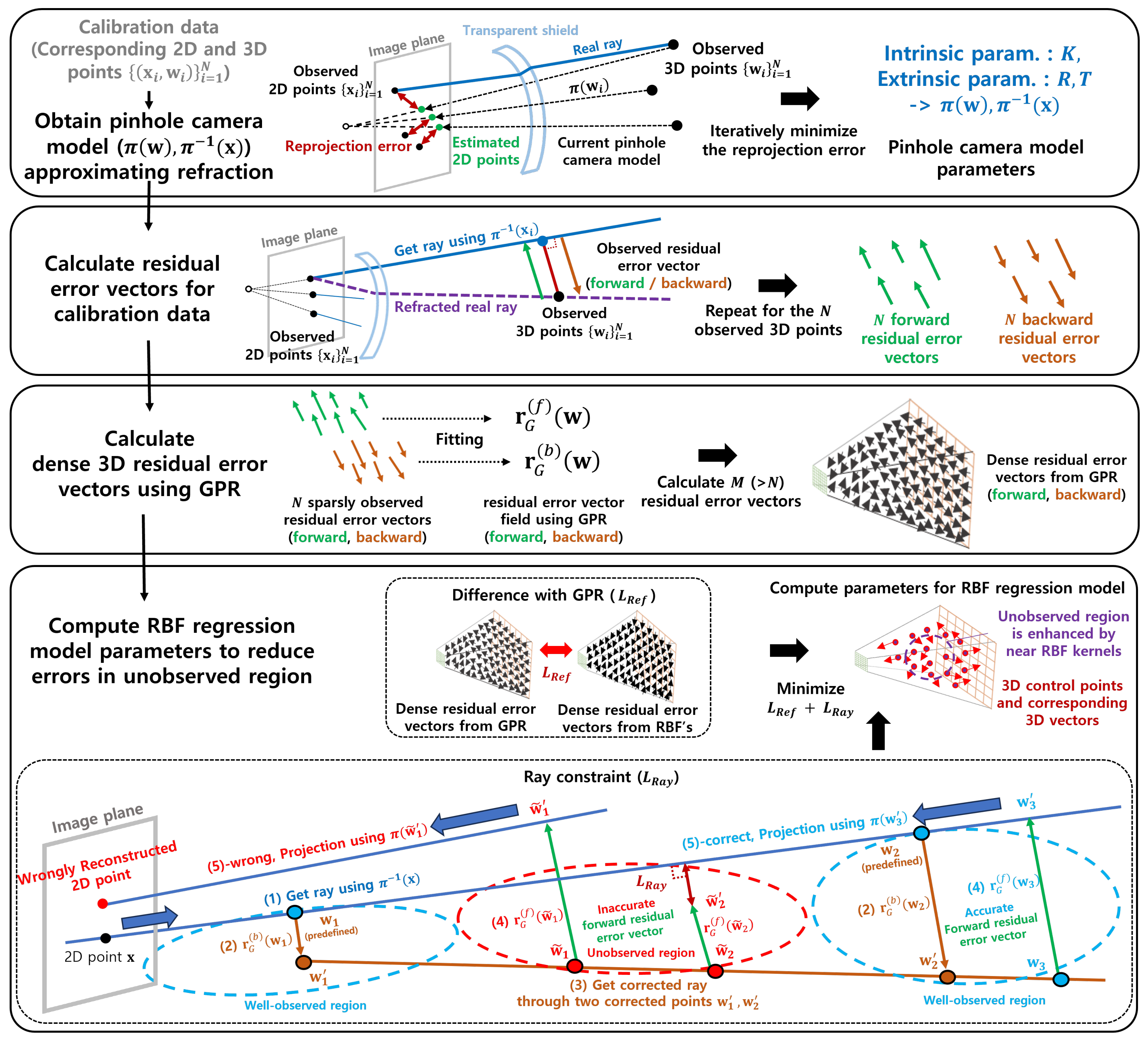
3. Methods
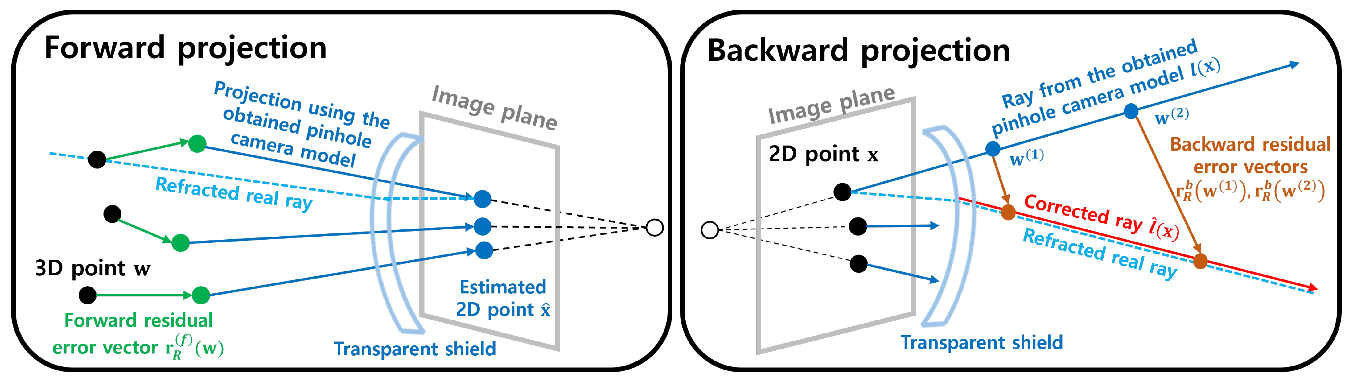
3.1. Residual Camera Model
3.2. Residual Error Vector Regression
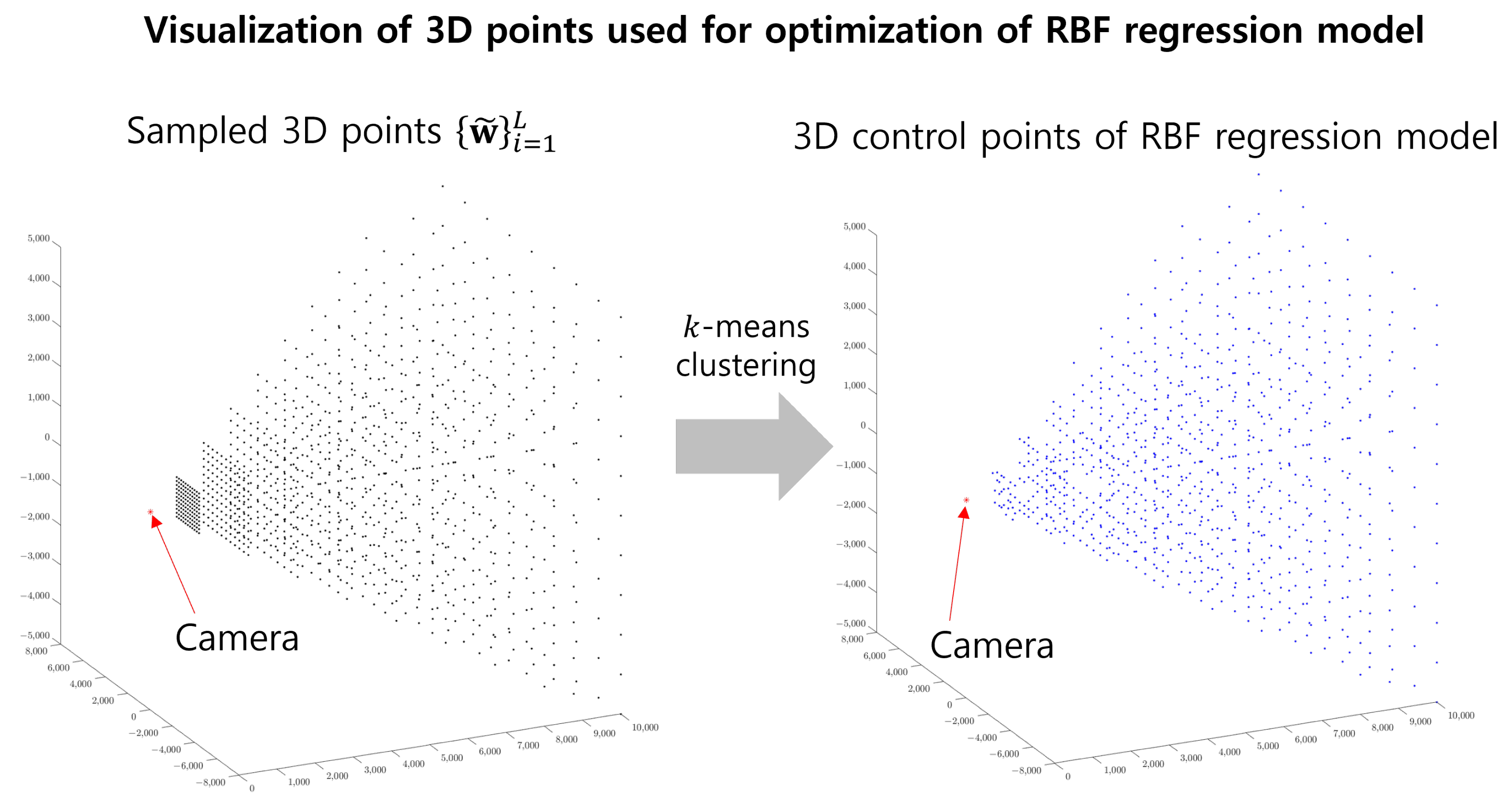
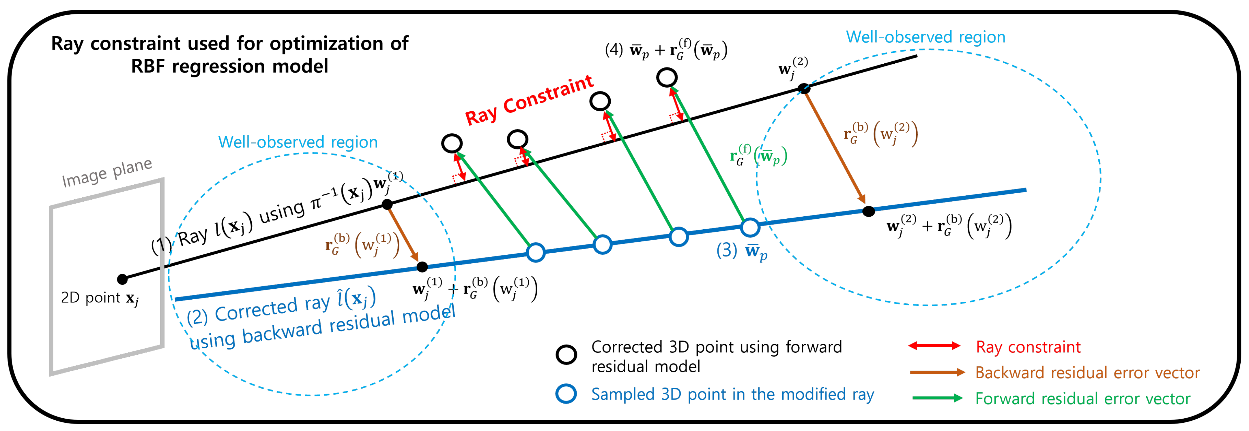
3.3. Optimization of the RBF Regression Model
3.3.1. Reference Objective
3.3.2. Ray Constraint
3.3.3. Combined Objective
4. Experiments
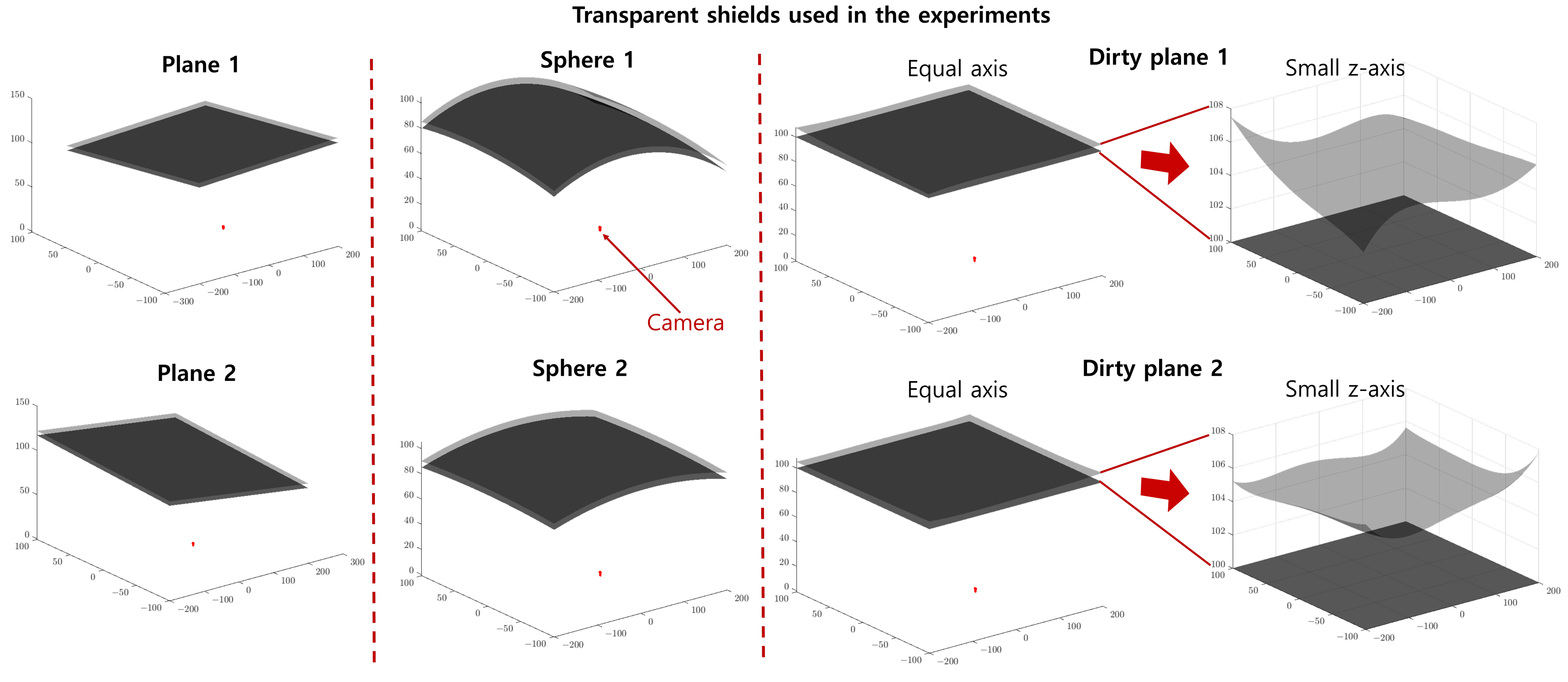
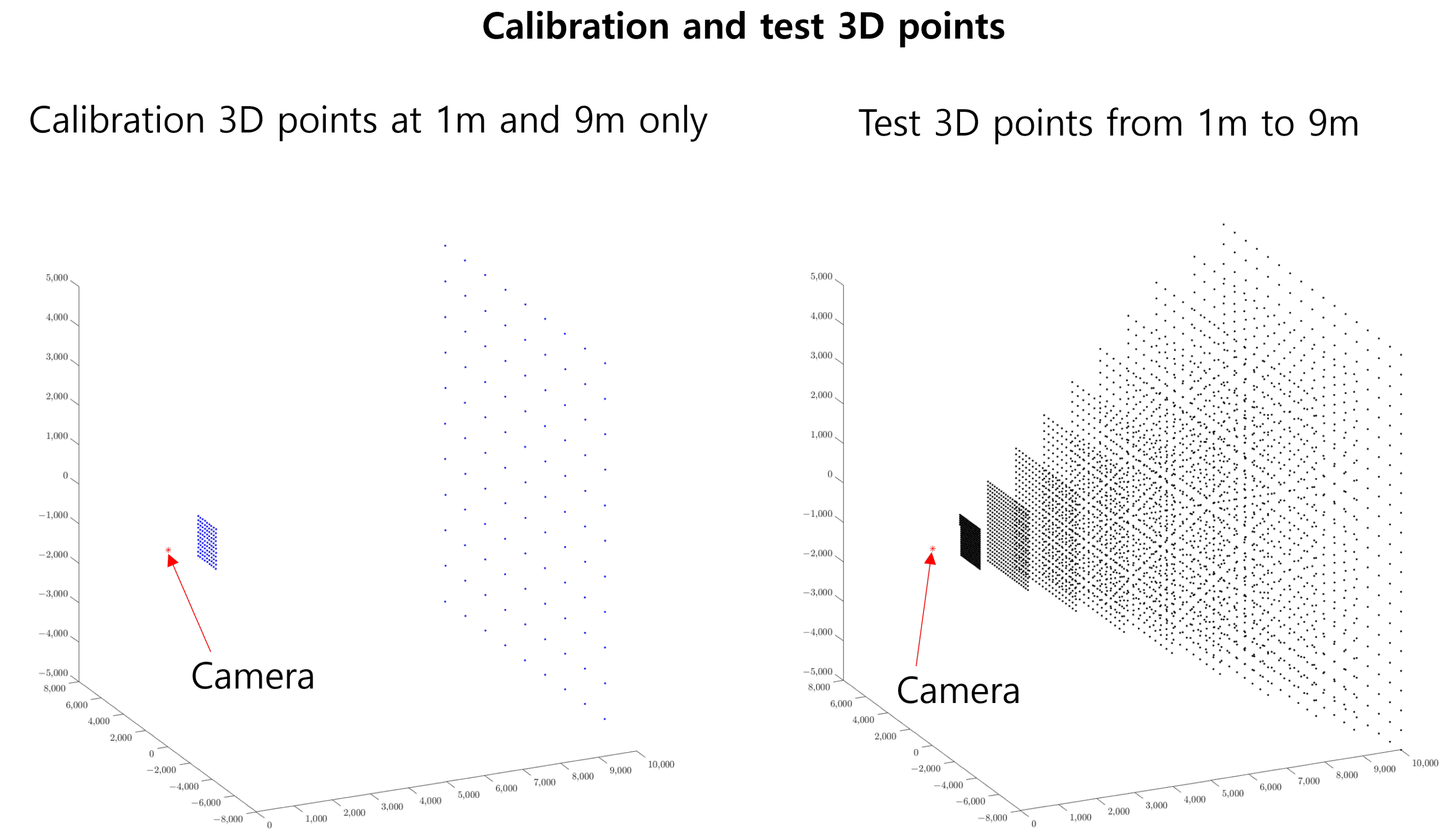
4.1. Dataset
4.2. Implementation Details
4.3. Evaluation Metric
4.4. Results along the Noise Levels
4.5. Results with Low Noise Levels
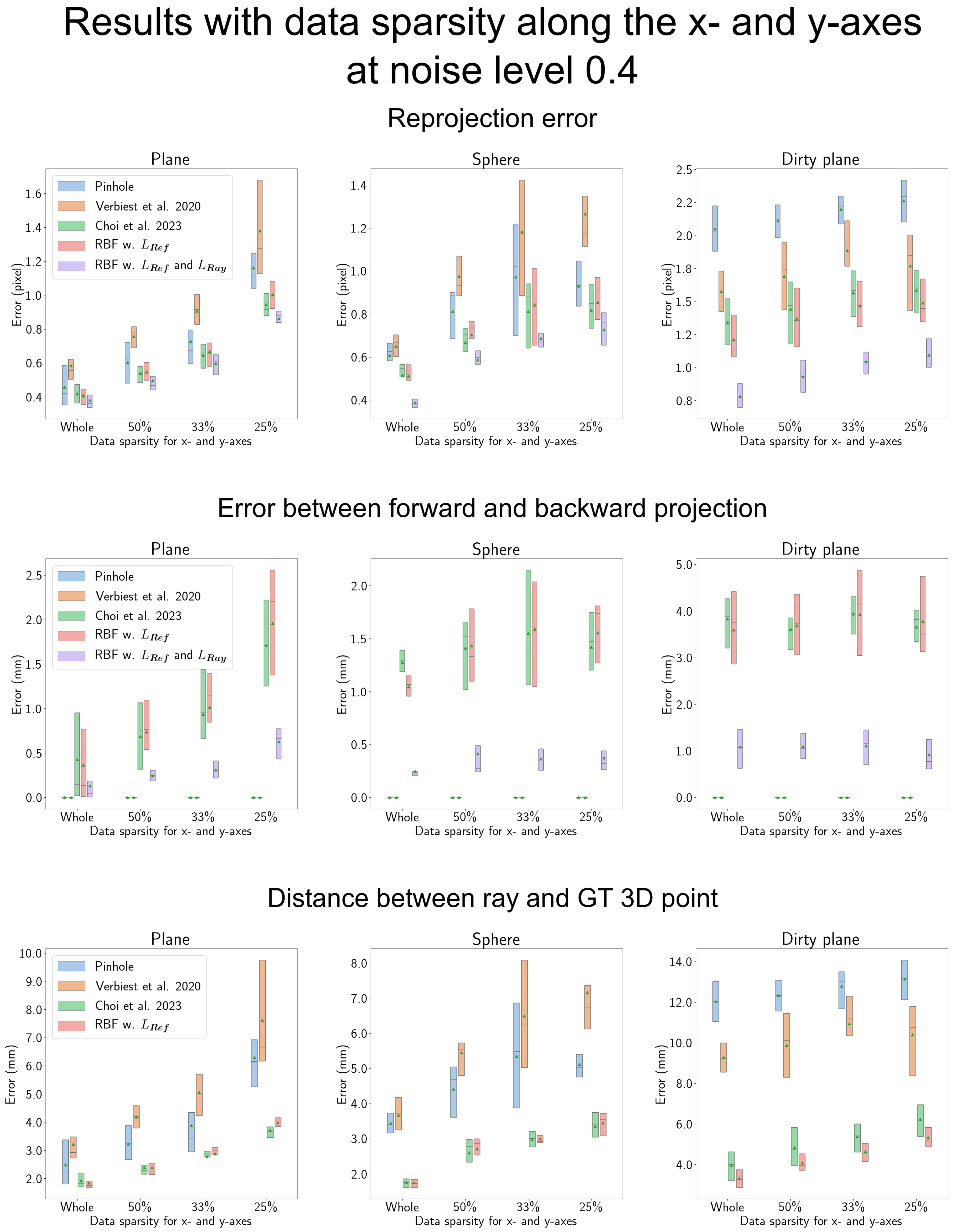
4.6. Results When the Data Are More Sparse along the x-, y-Axis
4.7. Ablation Study
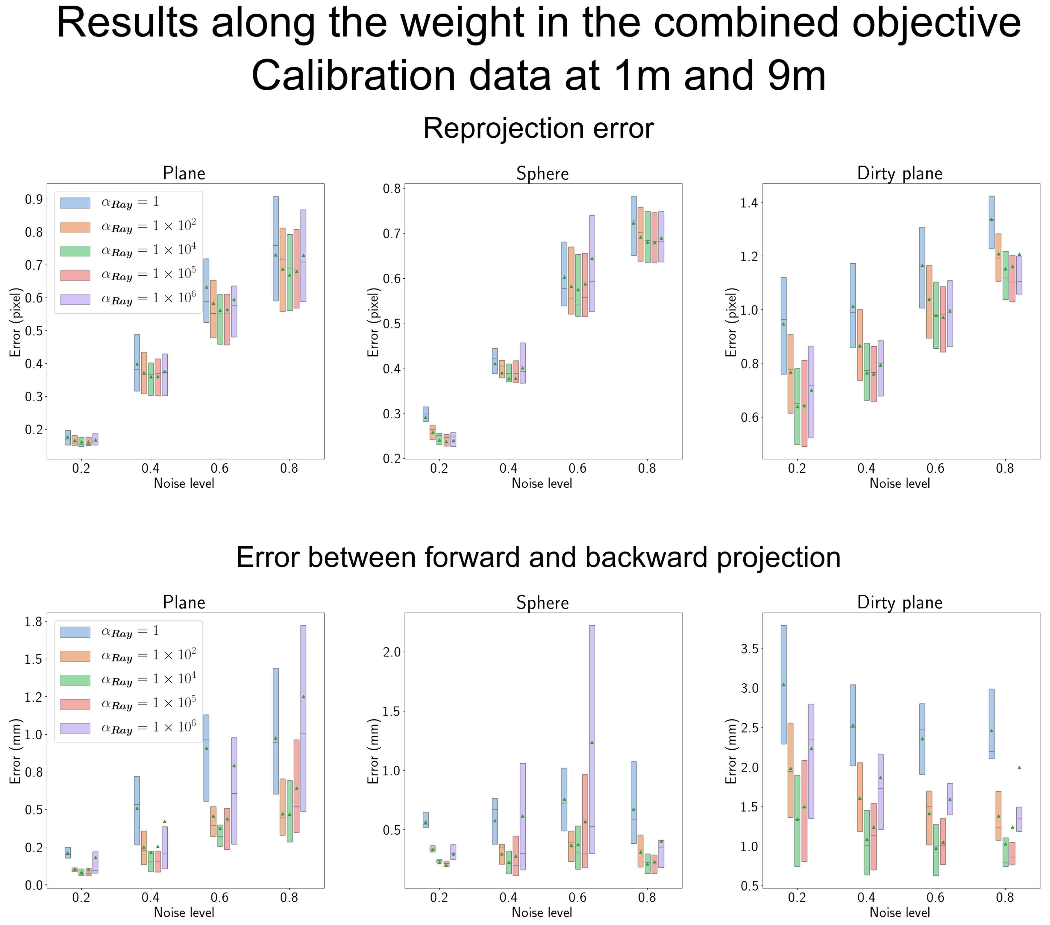
4.7.1. Results According to the Weight for the Ray Constraint in Section 3.3.3
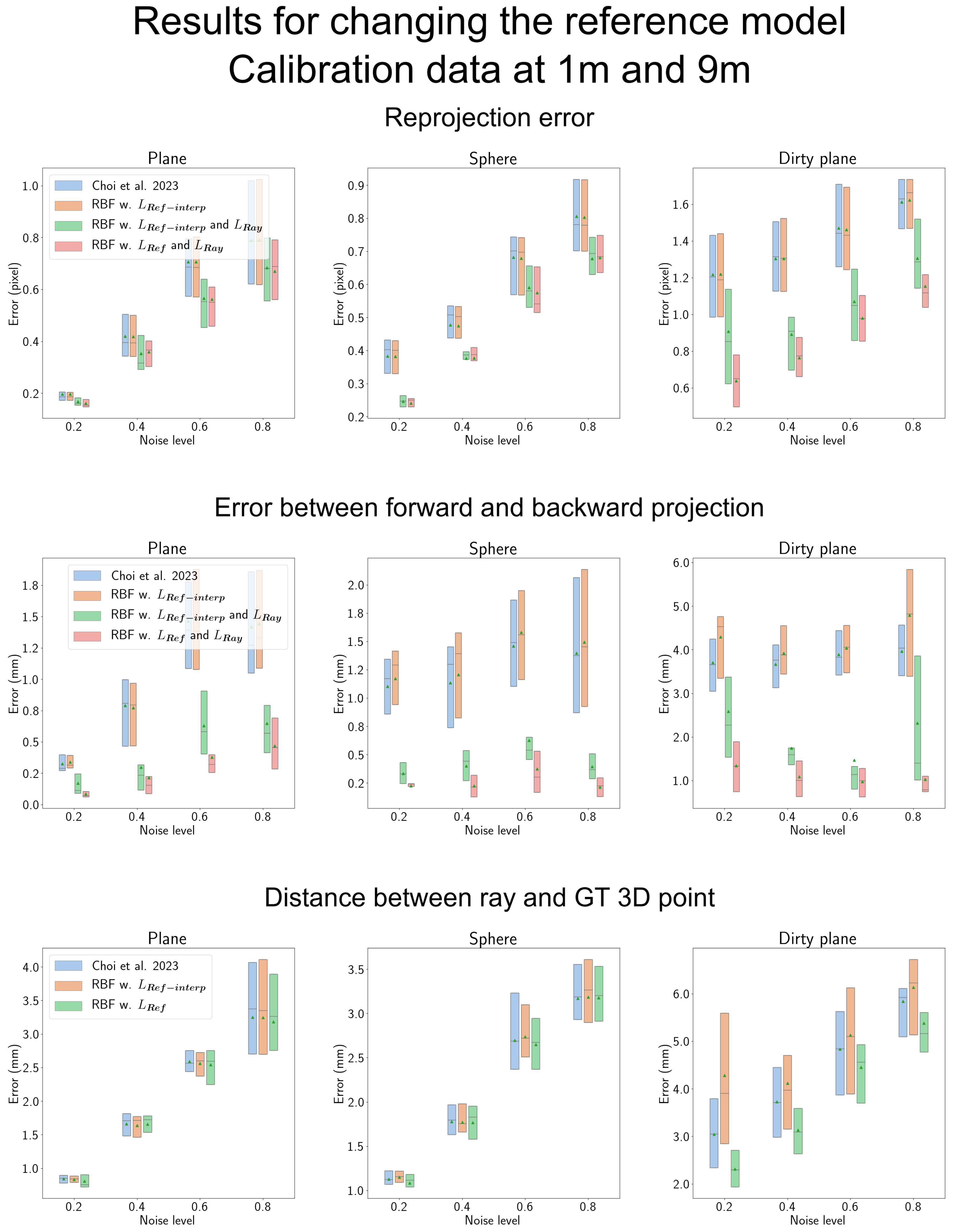
4.7.2. Results of Changing the Reference Model
4.7.3. Results According to the Data Sparsity along the z-Axis
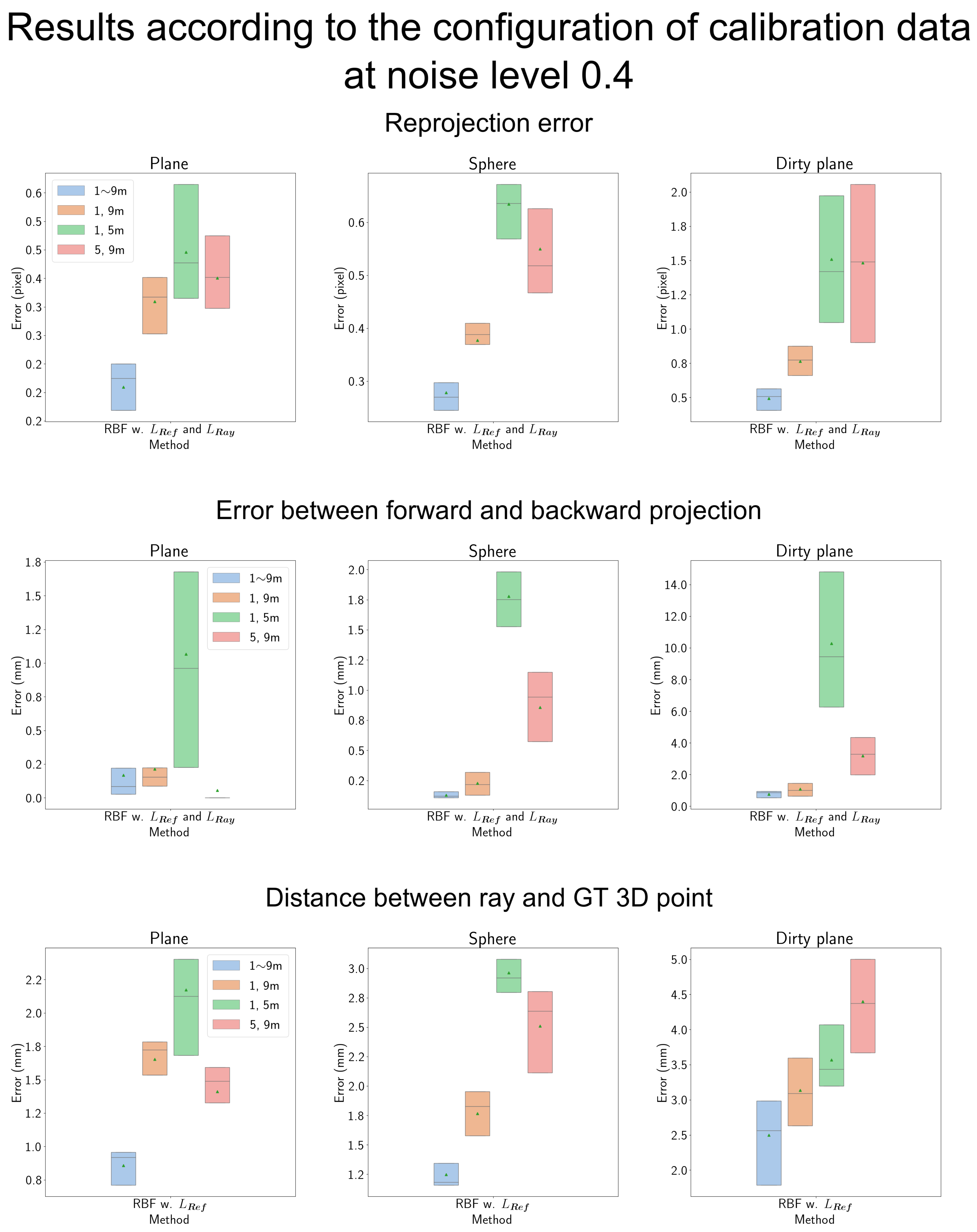
4.7.4. Results According to the Configuration of Calibration Data
4.7.5. Computational Load of the Proposed RBF-Based Camera Model
5. Limitations and Future Work
6. Conclusions
Author Contributions
Funding
Institutional Review Board Statement
Informed Consent Statement
Data Availability Statement
Conflicts of Interest
References
- Tourani, A.; Bavle, H.; Sanchez-Lopez, J.L.; Voos, H. Visual SLAM: What Are the Current Trends and What to Expect? Sensors 2022, 22, 9297. [Google Scholar] [CrossRef] [PubMed]
- Liu, H.; Liu, T.; Chen, Y.; Zhang, Z.; Li, Y.F. EHPE: Skeleton cues-based gaussian coordinate encoding for efficient human pose estimation. In IEEE Transactions on Multimedia; IEEE: Piscataway Township, NJ, USA, 2022. [Google Scholar]
- Kang, L.; Wu, L.; Yang, Y.H. Experimental study of the influence of refraction on underwater three-dimensional reconstruction using the svp camera model. Appl. Opt. 2012, 51, 7591–7603. [Google Scholar] [CrossRef] [PubMed]
- Pável, S.; Sándor, C.; Csató, L. Distortion estimation through explicit modeling of the refractive surface. In Proceedings of the Artificial Neural Networks and Machine Learning–ICANN 2019: Image Processing: 28th International Conference on Artificial Neural Networks, Munich, Germany, 17–19 September 2019; Springer: Berlin/Heidelberg, Germany, 2019; pp. 17–28. [Google Scholar]
- Cassidy, M.; Mélou, J.; Quéau, Y.; Lauze, F.; Durou, J.D. Refractive multi-view stereo. In Proceedings of the 2020 International Conference on 3D Vision (3DV), Fukuoka, Japan, 25–28 November 2020; IEEE: Piscataway Township, NJ, USA, 2020; pp. 384–393. [Google Scholar]
- Yoon, S.; Choi, T.; Sull, S. Depth estimation from stereo cameras through a curved transparent medium. Pattern Recognit. Lett. 2020, 129, 101–107. [Google Scholar] [CrossRef]
- Born, M.; Wolf, E. Principles of Optics: Electromagnetic Theory of Propagation, Interference and Diffraction of Light; Elsevier: Amsterdam, The Netherlands, 2013. [Google Scholar]
- Grossberg, M.D.; Nayar, S.K. A general imaging model and a method for finding its parameters. In Proceedings of the Eighth IEEE International Conference on Computer Vision. ICCV 2001, Vancouver, BC, Canada, 7–14 July 2001; IEEE: Piscataway Township, NJ, USA, 2001; Volume 2, pp. 108–115. [Google Scholar]
- Pless, R. Using many cameras as one. In Proceedings of the 2003 IEEE Computer Society Conference on Computer Vision and Pattern Recognition, Madison, WI, USA, 18–20 June 2003; IEEE: Piscataway Township, NJ, USA, 2003; Volume 2, p. II–587. [Google Scholar]
- Ramalingam, S.; Sturm, P. A unifying model for camera calibration. IEEE Trans. Pattern Anal. Mach. Intell. 2016, 39, 1309–1319. [Google Scholar] [CrossRef] [PubMed]
- Miraldo, P.; Araujo, H. Calibration of smooth camera models. IEEE Trans. Pattern Anal. Mach. Intell. 2012, 35, 2091–2103. [Google Scholar] [CrossRef] [PubMed]
- Beck, J.; Stiller, C. Generalized B-spline camera model. In Proceedings of the 2018 IEEE Intelligent Vehicles Symposium (IV), Changshu, China, 26–30 June 2018; IEEE: Piscataway Township, NJ, USA, 2018; pp. 2137–2142. [Google Scholar]
- Verbiest, F.; Proesmans, M.; Van Gool, L. Modeling the effects of windshield refraction for camera calibration. In Proceedings of the Computer Vision–ECCV 2020: 16th European Conference, Glasgow, UK, 23–28 August 2020; Springer: Berlin/Heidelberg, Germany, 2020; pp. 397–412. [Google Scholar]
- Choi, T.; Yoon, S.; Kim, J.; Sull, S. Noniterative Generalized Camera Model for Near-Central Camera System. Sensors 2023, 23, 5294. [Google Scholar] [CrossRef] [PubMed]
- Rosebrock, D.; Wahl, F.M. Generic camera calibration and modeling using spline surfaces. In Proceedings of the 2012 IEEE Intelligent Vehicles Symposium, Madrid, Spain, 3–7 June 2012; IEEE: Piscataway Township, NJ, USA, 2012; pp. 51–56. [Google Scholar]
- Zhang, Z. A flexible new technique for camera calibration. IEEE Trans. Pattern Anal. Mach. Intell. 2000, 22, 1330–1334. [Google Scholar] [CrossRef]
- Scaramuzza, D.; Martinelli, A.; Siegwart, R. A toolbox for easily calibrating omnidirectional cameras. In Proceedings of the 2006 IEEE/RSJ International Conference on Intelligent Robots and Systems (IROS), Beijing, China, 9–15 October 2006; pp. 5695–5701. [Google Scholar]
- Olson, E. AprilTag: A robust and flexible visual fiducial system. In Proceedings of the 2011 IEEE international conference on robotics and automation, Shanghai, China, 9–13 May 2011; IEEE: Piscataway Township, NJ, USA, 2011; pp. 3400–3407. [Google Scholar]
- Zhang, Z. Camera calibration with one-dimensional objects. IEEE Trans. Pattern Anal. Mach. Intell. 2004, 26, 892–899. [Google Scholar] [CrossRef]
- Bukhari, F.; Dailey, M.N. Automatic radial distortion estimation from a single image. J. Math. Imaging Vis. 2013, 45, 31–45. [Google Scholar] [CrossRef]
- Kakani, V.; Kim, H.; Lee, J.; Ryu, C.; Kumbham, M. Automatic distortion rectification of wide-angle images using outlier refinement for streamlining vision tasks. Sensors 2020, 20, 894. [Google Scholar] [CrossRef] [PubMed]
- Geyer, C.; Daniilidis, K. A unifying theory for central panoramic systems and practical implications. In Proceedings of the Computer Vision—ECCV 2000: 6th European Conference on Computer Vision, Dublin, Ireland, 26 June–1 July 2000; Springer: Berlin/Heidelberg, Germany, 2000; pp. 445–461. [Google Scholar]
- Rosebrock, D.; Wahl, F.M. Complete generic camera calibration and modeling using spline surfaces. In Proceedings of the Asian Conference on Computer Vision, Daejeon, Republic of Korea, 5–9 November 2012; Springer: Berlin/Heidelberg, Germany, 2012; pp. 487–498. [Google Scholar]
- Schops, T.; Larsson, V.; Pollefeys, M.; Sattler, T. Why having 10,000 parameters in your camera model is better than twelve. In Proceedings of the IEEE/CVF Conference on Computer Vision and Pattern Recognition, Seattle, WA, USA, 13–19 June 2020; pp. 2535–2544. [Google Scholar]
- Miraldo, P.; Araujo, H.; Queiro, J. Point-based calibration using a parametric representation of the general imaging model. In Proceedings of the 2011 International Conference on Computer Vision, Barcelona, Spain, 6–13 November 2011; IEEE: Piscataway Township, NJ, USA, 2011; pp. 2304–2311. [Google Scholar]
- Majdisova, Z.; Skala, V. Radial basis function approximations: Comparison and applications. Appl. Math. Model. 2017, 51, 728–743. [Google Scholar] [CrossRef]
- MATLAB. Version: 9.14.0.2286388 (R2023a) Update 3; The MathWorks Inc.: Natick, MA, USA, 2023. [Google Scholar]


| Abbreviation | Full Version of the Phrase |
|---|---|
| RBF | Radial Basis Function |
| GPR | Gaussian Process Regression |
| GT | Ground Truth |
| 3D | Three-dimensional |
| 2D | Two-dimensional |
| Method | Computation Time (ms) | |
|---|---|---|
| Forward Projection | Backward Projection | |
| Miraldo et al. [11] | 20,887.9 ± 471.1 | 96.4 ± 2.0 |
| Verbiest et al. [13] | 32.9 ± 4.0 | 44,355.7 ± 1060.6 |
| Choi et al. [14] | 32.3 ± 0.5 | 63.9 ± 0.8 |
| Proposed | 60.6 ± 2.4 | 120.4 ± 1.6 |
Disclaimer/Publisher’s Note: The statements, opinions and data contained in all publications are solely those of the individual author(s) and contributor(s) and not of MDPI and/or the editor(s). MDPI and/or the editor(s) disclaim responsibility for any injury to people or property resulting from any ideas, methods, instructions or products referred to in the content. |
© 2023 by the authors. Licensee MDPI, Basel, Switzerland. This article is an open access article distributed under the terms and conditions of the Creative Commons Attribution (CC BY) license (https://creativecommons.org/licenses/by/4.0/).
Share and Cite
Kim, J.; Kim, C.; Yoon, S.; Choi, T.; Sull, S. RBF-Based Camera Model Based on a Ray Constraint to Compensate for Refraction Error. Sensors 2023, 23, 8430. https://doi.org/10.3390/s23208430
Kim J, Kim C, Yoon S, Choi T, Sull S. RBF-Based Camera Model Based on a Ray Constraint to Compensate for Refraction Error. Sensors. 2023; 23(20):8430. https://doi.org/10.3390/s23208430
Chicago/Turabian StyleKim, Jaehyun, Chanyoung Kim, Seongwook Yoon, Taehyeon Choi, and Sanghoon Sull. 2023. "RBF-Based Camera Model Based on a Ray Constraint to Compensate for Refraction Error" Sensors 23, no. 20: 8430. https://doi.org/10.3390/s23208430
APA StyleKim, J., Kim, C., Yoon, S., Choi, T., & Sull, S. (2023). RBF-Based Camera Model Based on a Ray Constraint to Compensate for Refraction Error. Sensors, 23(20), 8430. https://doi.org/10.3390/s23208430