Abstract
This paper presents the design, optimization, and calibration of multivariable resonators for microwave dielectric sensors. An optimization technique for the circular complementary split ring resonator (CC-SRR) and square complementary split ring resonator (SC-SRR) is presented to achieve the required transmission response in a precise manner. The optimized resonators are manufactured using a standard photolithographic technique and measured for fabrication tolerance. The fabricated sensor is presented for the high-resolution characterization of dielectric substrates and oil samples. A three-dimensional dielectric container is attached to the sensor and acts as a pool for the sample under test (SUT). In the presented technique, the dielectric substrates and oil samples can interact directly with the electromagnetic (EM) field emitted from the resonator. For the sake of sensor calibration, a relation between the relative permittivity of the dielectric samples and the resonant frequency of the sensor is established in the form of an inverse regression model. Comparisons with state-of-the-art sensors indicate the superiority of the presented design in terms of oil characterization reliability. The significant technical contributions of this work include the employment of the rigorous optimization of geometry parameters of the sensor, leading to its superior performance, and the development and application of the inverse-model-based calibration procedure.
1. Introduction
Metamaterials (MTMs) play a vital role in the development of microwave sensors. MTMs are artificially engineered electromagnetic materials in which metallic elements are arranged periodically to achieve extraordinary properties unavailable in conventional materials [1]. MTMs are classified into two categories: non-resonant and resonant. The non-resonant MTM technique, which is based on the transmission lines, was initially proposed by Iyer et al. [2], A. Oliner [3], and C. Caloz et al. [4] to achieve a negative refractive index medium and artificial left-handed materials. The resonant MTM technique is based on sub-wavelength resonant components such as split ring resonators (SRR) [5] and complementary split ring resonators (CSRR) [6]. The SRR was proposed by John Pendry et al. [7] as a resonant magnetic particle capable of achieving effective negative permeability. The CSRR is a dual counterpart of SRR and was proposed by F. Falcone et al. [8] as an effective negative permittivity resonator in 2004. In the following year, J.D. Baena et al. [9] introduced the equivalent circuit for the CSRR, which was based on lumped elements, that has since gained widespread acceptance. It has been demonstrated that CSRR can be excited by external electric and magnetic fields to exhibit a cross-polarization effect. This concept has been utilized to design a metasheet for transmission polarization [10], miniature antennas [11], waveguide passband filters [12], and microstrip stopband filters [13]. Later on, these filtering characteristics were used for microwave sensing applications [14].
Recently, CSRR-based microwave sensors have begun to attract renewed interest in the real-time characterization of microfluidic and solid materials [15,16,17,18,19,20,21,22,23,24]. This analysis is based on the alteration of the transmission response of the CSRR, more specifically, changing the operating parameters (resonant frequency, notch depth, and quality factor) due to its interaction with the sample under test (SUT). In [15], a CSRR was used to characterize high-energy materials with a resonant frequency (fr) of 4.48 GHz and a minimum frequency shift (Δfmin) of 20 MHz. The CSRR was applied in [16] to analyze a water-ethanol mixture with a fr of 2.35 GHz and a Δfmin of 50 MHz. In another study [17], a quasi-static CSRR was used for the nondestructive thickness measurement of Teflon films, with a fr of 2.3 GHz and a Δfmin of 151 MHz. In [18], an ethanol chemical sensor was proposed that employs a CSRR-loaded patch with a fr of 4.16 GHz and a Δfmin of 300 MHz. In another study [19], a square-shaped CSRR was utilized to measure the thickness of multilayer dielectric substrates with a fr of 3.83 GHz and a Δfmin of 348 MHz. In [20], a CSRR connected to a microstrip line was employed for microfluidic dielectric characterization with a fr of 2 GHz and a Δfmin of 400 MHz. In another study [21], a dual-band sensor was designed using a single compound CSRR to evaluate the thickness of dielectric substrates with an average error of 6.26 percent. In [22], two CSRRs were used for the noninvasive measurement of glucose levels with a concentration of 0 to 400 mg/dL, featuring a sensitivity of 0.03 dB per mg/mL. In another study [23], a multiple-squares CSRR-loaded flared patch was introduced to evaluate the oils, with a fr of 8.49 GHz and a Δfmin of 885 MHz. In [24], a square CSRR-loaded microstrip patch was presented to evaluate edible oils, with a fr of 9.80 GHz and a Δfmin of 1133 MHz. The aforementioned microwave sensors were designed to operate at frequencies lower than 10 GHz to avoid fabrication and measurement challenges. Notwithstanding, the sensor’s resonant frequency, sensitivity, and range of applicability are highly dependent on the appropriate sizing of the circuit dimensions. Typically, the sensitivity of microwave sensors based on CSRR is determined by the resonant frequency, the material properties of the SUT, and the interaction of the SUT with the CSRR’s electromagnetic field. When designing a high-sensitivity sensor, these three parameters are to be considered while staying within the fabrication and measurement limits. Interactive methods such as parameter sweeping are used in practice to realize the tuning of parameters [25,26]. In [25], the parametric sweep method was used to study the effects of resonator dimensions on the resonance frequency and notch depth of a filter by varying one parameter while holding the others constant. In [26], four geometric parameters were utilized to tune the resonant frequency of the CSRR, utilizing the parametric sweep technique. This method is computationally inefficient since it requires a full electromagnetic (EM) wave simulation for each geometrical parameter combination, which is a time-consuming process. This method involves the designer’s direct participation to produce the desired outcomes, resulting in suboptimal results. Therefore, an optimization approach is required to simultaneously manage numerous geometric factors and to fulfill several objectives (such as frequency allocation and depth control).
In this paper, a technique is proposed for optimizing a circular complementary split ring resonator (CC-SRR) and square complementary split ring resonator (SC-SRR) linked to microstrip transmission lines. The optimization method is developed to precisely assign the operating frequency of the device while enhancing the resonator’s quality factor. In addition to being generic, the approach is distinguished by its computational efficiency. The CC-SRR and SC-SRR are tuned to resonate at 15 GHz to detect changes in the sample’s permittivity, permeability, dielectric, and magnetic loss tangents. The application case study is the prime motivation for choosing 15 GHz as the operating frequency. In the design of microwave sensors, the relative permittivity of the test sample is crucial. For instance, microwave sensors have been built to operate between frequencies of 1 GHz and 6 GHz for measuring samples with high relative permittivity values (εr = 20 to 82) [27,28,29]. Microwave sensors are commonly built for frequencies between 7 GHz and 14 GHz for the characterization of samples with medium relative permittivity values (εr = 4 to 20) [30,31] and between 14 GHz and 30 GHz for the measurement of low permittivity materials (εr = 1 to 4) [32,33]. These examples demonstrate that, depending on the anticipated material qualities of the samples being tested, the required resonant frequency of the sensor may vary significantly. To reliably evaluate oils with a relative permittivity between 2.20 and 3.08, a resonator with a high degree of sensitivity is required. Despite the fact that the challenge of fabrication tolerance is amplified by this high sensitivity. We calibrated our sensor after fabrication to prevent fabrication tolerance from affecting the relative permittivity measurement of oils in order to solve this problem. Both sensors are manufactured using a standard photolithographic procedure and measured using a Rohde & Schwarz ZNB20 vector network analyzer. To establish the fabrication tolerance of the CC-SRR and SC-SRR, the simulated and measured transmission coefficients of the unloaded sensors are compared. According to the comparison, the SC-SRR has a low fabrication sensitivity and outstanding accuracy, making it suitable for the high-resolution characterization of dielectric substrates and oil samples. A polylactide acid (PLA) container is placed over the SC-SRR in the ground plane to confine the oil under test (OUT) and to enable its interaction with the electromagnetic (EM) field emitted from the SC-SRR. Furthermore, upon calibration, a closed-form analytical expression is derived which allows for direct extraction of the OUT’s relative permittivity by measuring the sensor’s real-time transmission response due to interaction with the OUT.
The main contribution of this paper is a rapid design optimization technique based on surrogate modeling of geometric parameters that outperforms the parameter sweep method, the latter being commonly used in practice to achieve parameter tuning. In fact, identifying an optimal design using parameter sweeping is impossible given a few parameters and various objectives (for example, frequency allocation of the resonance and managing its depth). In contrast, the method provided in this paper can control both objectives, handle several geometry parameters at the same time, and is provably convergent. Furthermore, it has demonstrated the ability to produce sensors with high sensitivity and less measurement error comparable to state-of-the-art circuits.
2. Design and Optimization
Two microwave sensors are designed using a circular complementary split ring resonator (CC-SRR) and a square complementary split ring resonator (SC-SRR) connected to a microstrip transmission line (MTL). As illustrated in Figure 1, each sensor is implemented on a RO4003C substrate with a relative permittivity εr = 3.38 ± 0.05, length sl = 30 mm, width sw = 25 mm, and height sh = 0.813 mm. The MTL is printed on the top layer of the RO4003C substrate, whereas the CC-SRR and SC-SRR are etched into the bottom layer of each sensor. The following equations are used to optimize the size of the MTL in order to create a 50-ohm sensor impedance that matches the impedance of the vector network analyzer [34].
where εre = 2.67 is the effective dielectric constant of the MTL, η = 120π Ω is the impedance of the wave in free space, and the optimized width of the MTL is mw = 1.88 mm. Figure 1b depicts the electromagnetic field generated by the MTL as a result of waveguide port excitation. Five independent variables explain the geometry of CC-SRR, as illustrated in Figure 1c: a1 (outer diameter of the outer circle), b1 (inner diameter of the outer circle), c1 (outer diameter of the inner circle), d1 (inner diameter of the inner circle), and e1 (size of the splits in each circle). As shown in Figure 1d, the geometry of the SC-SRR is described by five parameters: a2 (outer length of the outer square), b2 (inner length of the outer square), c2 (inner length of the inner square), d2 (outer length of the inner square), and e2 (size of the splits in each square).
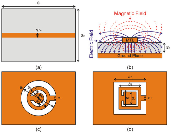
Figure 1.
(a) Top view of the sensor based on the RO4003C substrate and microstrip transmission line (MTL), (b) Electromagnetic fields created by the MTL, (c) Geometry of the optimized CC-SRR, and (d) Geometry of the optimized SC-SRR.
The initial (prior to optimization) geometric values for the CC-SRR and SC-SRR are a1 = a2 = 2 mm, b1 = b2 = 1.6 mm, c1 = c2 = 1.2 mm, d1 = d1 = 0.8 mm, and e1 = e2 = 0.2 mm. In CST Microwave Studio, each sensor is simulated using the hexahedral finite integration technique (FIT) solver, and the simulated transmission coefficients (S21) are shown in Figure 2. According to the simulation results, the CC-SRR has a resonance frequency of 16.72 GHz and a notch depth of −23.19 dB, whereas the SC-SRR has a resonance frequency of 13.77 GHz and a notch depth of −24.58 dB.
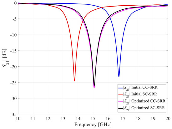
Figure 2.
Simulated transmission coefficients for the initial and optimized CC-SRR and SC-SRR.
For parametric studies, one parameter is changed at one time while keeping other parameters at their reference values. For this purpose, the CC-SRR is described by variables w1, w2, w3, and w4, whereas the SC-SRR is specified by w5, w6, w7, and w8. Where w1 = e1 = 0.2 mm is the width of the splits for CC-SRR, w2 = c1 − d1/2 = 0.2 mm is the width of the inner ring for CC-SRR, w3 = b1 − c1/2 = 0.2 mm is the width of copper metal between the inner ring and outer ring for CC-SRR, w4 = a1 − b1/2 = 0.2 mm is the width of the outer ring for CC-SRR, w5 = e2 = 0.2 mm is the width of the splits for SC-SRR, w6 = c2 − d2/2 = 0.2 mm is the width of the inner ring for SC-SRR, w7 = b2 − c2/2 = 0.2 mm is the width of copper metal between the inner ring and outer ring for SC-SRR, and w8 = a2 − b2/2 = 0.2 mm is the width of the outer ring for CC-SRR. The resonant frequency and the notch depth of the CC-SRR and SC-SRR sensors as a result of design parameter variations are shown in Figure 3 and Figure 4, respectively. In these figures, as mentioned earlier, one parameter of each structure is changed at one time while keeping other parameters at their reference values. For example, when the parameter w1 is changed from 0.2 mm to 1 mm with the step of 0.1 mm, other parameters are kept at their reference values, w2 = w3 = w4 = 0.2 mm.
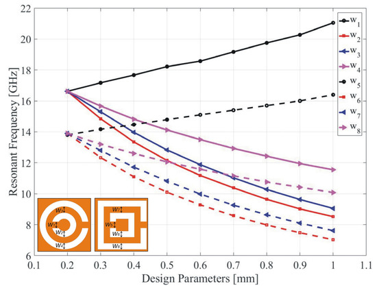
Figure 3.
Variation in resonant frequency due to changes in the design parameters of CC-SRR (w1, w2, w3, and w4) and SC-SRR (w5, w6, w7, and w8).
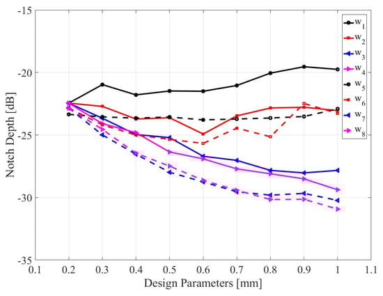
Figure 4.
Variation in notch depth due to changes in the design parameters of CC-SRR (w1, w2, w3, and w4) and SC-SRR (w5, w6, w7, and w8).
It can be observed that due to a relatively large number of variables and their joint effects on both the frequency location and the depth of the notch, identifying the optimum solution with respect to the assumed requirements (here, the precise allocation of the notch at the target frequency and maximization of the depth at the same time) is virtually impossible. Further, repetitive sweeps entail considerable computational expenditures due to the massive EM simulations necessary for each tested combination of the parameters. Parameter interdependence, the need for controlling more than one objective at a time, makes simultaneous parameter adjustment imperative, which can only be achieved by means of rigorous numerical optimization techniques.
For the purpose of optimization, the geometric parameters are aggregated into a vector x = [an bn cn dn en]T, where n = 1 for the CC-SRR and n = 2 for the SC-SRR. We are concerned with the resonance frequency of the first notch, denoted as f0. We also denote as L0 the level of transmission |S21| at f0.
The design optimization task is formulated as:
where x* is the optimum design to be identified and ft is the target notch frequency.
The objective function is defined as:
Its first term is the primary objective (increasing the depth of the resonance), whereas the second term is a penalty function used to enforce and allocate the resonant frequency near the target ft. Here, we set ft = 15 GHz. The optimization process is carried out using a trust-region gradient-based algorithm with numerical derivatives [35], which is accelerated using the rank-one Broyden update [36] to reduce the computational cost of the process. Owing to this arrangement, the parameter tuning process is low cost and corresponds to less than thirty EM analyses of the circuit under design. More importantly, the particular formulation problem and the associated definition of the objective function (4) allow for the simultaneous adjustment of all relevant geometry parameters and control over the operating frequency of the structure and the notch depth. Neither of these would be possible using the traditional method, e.g., based on experience-driven parametric studies. Further, the process is fully automated, whereas its computational efficiency cannot be matched by hands-on methods.
The optimization process of CC-SRR leads to a1 = 2.467 mm, b1 = 1.726 mm, c1 = 1.191 mm, d1 = 0.810 mm, and e1 = 0.359 mm. The obtained notch depth is –26.67 dB, with the resonant frequency being 15.08 GHz. The SC-SRR optimization results in a2 = 2.073 mm, b2 = 1.412 mm, c2 = 1.052 mm, d2 = 0.814 mm, and e2 = 0.336 mm. The notch depth observed is –26 dB and the resonant frequency is 15.08 GHz. Although the optimized resonators have different geometric shapes but the same transmission coefficients, as shown in Figure 2, they can be referred to as equivalent resonators. The optimized resonators have unequal widths in both rings as shown in Figure 1, which distinguishes them from conventional resonators in the literature and affects their sensitivity, which will be discussed in the following section.
3. Sensitivity Analysis
The optimized sensors undergo sensitivity analysis by perturbing the SUT’s volume and electromagnetic properties. According to the perturbation technique, the change in resonance frequency (∆fr) of the sensor is proportional to the perturbed volume (dυ), the change in permeability (∆µ), and the permittivity (∆ε) of the SUT. The following equation expresses the fractional change in the resonant frequency of the sensor [37]:
This equation indicates that any increase in the volume, permeability, or permittivity of the SUT will decrease the sensor’s resonant frequency. For volume perturbation, a sample under test (SUT) is placed on the CC-SRR and SC-SRR in each sensor’s ground plane, as illustrated in Figure 5. Because the CC-SRR and SC-SRR are etched out of the ground plane’s copper layer (17.5 μm), there is an air gap between the substrate and the SUT in the shape of resonators, which is taken into account in modeling. A RO4003C substrate with relative permittivity εr = 3.38 ± 0.05 is utilized as the SUT (h1 = 5 mm and h2 = 5 mm) and the volume of the SUT is changed by altering the thickness (h3 = 0.1 mm to 1.5 mm) of the RO4003C substrate. Figure 6 shows that the change in resonance frequency is inversely related to the SUT’s thickness up to 1 mm; beyond that, the influence of the SUT’s thickness begins to diminish, and for thickness larger than 1.5 mm, the resonance frequency is saturated. Table 1 summarizes the effect of the SUT’s thickness on the resonance frequency, bandwidth, and loaded Q factor of the CC-SRR and SC-SRR sensors. Increasing the thickness of the SUT reduces the resonant frequency and bandwidth while increasing the sensor’s Q factor. The SC-SRR sensor’s frequency change is larger than that of the CC-SRR sensor, showing that the SC-SRR is more sensitive to changes in the SUT’s thickness.
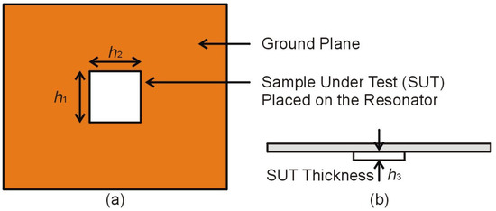
Figure 5.
The sensor’s ground plane contains the sample under test (SUT) which interacts with the electromagnetic fields created by the microstrip transmission line and radiated by the resonator, (a) Top View (b) Front View.
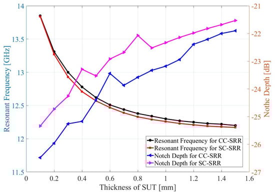
Figure 6.
Effect of the SUT’s thickness on CC-SRR and SC-SRR sensors’ resonance frequency and notch depth.

Table 1.
The influence of the SUT’s thickness on the resonant frequency, bandwidth, and Loaded Q factor of the CC-SRR and SC-SRR sensors.
For electromagnetic properties perturbation, the volume of the SUT is kept constant (h1 = 5 mm, h2 = 5 mm, and h3 = 1 mm) and the permittivity (εr), permeability (μr), dielectric loss tangent (tanδe), and magnetic loss tangent (tanδm) of the SUT is varied as tabulated in Table 2. According to Table 2, the εr and μr of the SUT affect the resonance frequency of the sensors while the tanδe and tanδm of the SUT influence the notch depth of the sensors. Figure 7 and Figure 8 show the effect of the SUT’s electromagnetic properties on the transmission coefficients of the CC-SRR and SC-SRR sensors. Only numerical simulations can reveal the individual effect of electromagnetic characteristics, as shown in Figure 7 and Figure 8. The effect of multiple combinations of EM properties can be seen in measurements where dielectric materials are primarily determined by their relative permittivity; the magnetic permeability is typically one and loss tangents are near zero. The resonator’s high resonance frequency and narrow bandwidth are critical to the performance of a microwave sensor. By optimizing geometrical parameters, the transmission response of both CC-SRR and SC-SRR resonators is made equivalent (same resonance frequency and bandwidth). The size of the resonator is the next factor that influences performance; a smaller size results in a stronger electromagnetic field that interacts with the SUT. Because the optimized SC-SRR is smaller in size than the CC-SRR, it outperforms its circular equivalent in performance.
Table 2.
The influence of the electromagnetic properties of the SUT on the resonance frequency and notch depth of the CC-SRR and SC-SRR sensors.
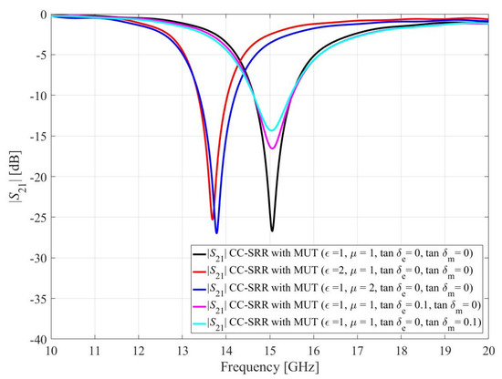
Figure 7.
Simulated transmission coefficients (S21) of the CC-SRR due to interaction with the sample under test (SUT) by perturbing one of SUT’s electromagnetic parameters.
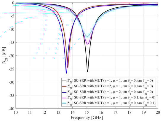
Figure 8.
Simulated transmission coefficients (S21) of the SC-SRR due to interaction with the sample under test (SUT) by perturbing one of SUT’s electromagnetic parameters.
4. Fabrication and Measurement
The optimized sensors have been fabricated using the chemical etching process on a double-sided copper-clad laminated (17.5 μm) RO4003C substrate, cf. Figure 9. The dimensions of the substrate, microstrip transmission line, and the optimized CC-SRR and SC-SRR are the same as mentioned in the optimization section. To measure the transmission response (S21), the fabricated sensors are connected to the vector network analyzer (Rohde & Schwarz ZNB20) using 2.92 mm end launch connectors. As illustrated in Figure 9, the simulation model is implemented using 2.92 mm end launch connectors to determine the influence of end launch connectors on the S21 of the optimized sensors. The simulated and measured S21 of the optimized sensors with end launch connectors is shown in Figure 10. The CC-SRR and SC-SRR sensors with end launch connectors have the simulated resonant frequencies of 15.05 GHz with a notch depth of −26.59 dB and 15.07 GHz with a notch depth of −26.16 dB, respectively. For the CC-SRR sensor, the difference between the simulated resonant frequencies with and without end launch connectors is 0.03 GHz, whereas, for the SC-SRR sensor, it is 0.01 GHz. The effect of end launch connectors on resonant frequencies is negligible, although the simulation takes five times longer than with sensors without end launch connectors. The measured resonant frequencies of the CC-SRR and SC-SRR sensors are 14.51 GHz with a notch depth of −19.83 dB and 14.62 GHz with a notch depth of −21.4 dB, respectively. For the CC-SRR sensor, the difference between the simulated and measured resonant frequencies is 3.65%, while for the SC-SRR sensor, it is 3.03%. The better fabrication tolerance of the SC-SRR is due to the structural shape of the resonator. In general, circular shapes are more susceptible to fabrication than square shapes, as demonstrated by our findings. To ensure the consistency of the measured data, each sensor is manufactured twice using the same procedure, and the results are similar. The measured result indicates that the SC-SRR has a good fabrication tolerance than the CC-SRR; therefore, it is calibrated for practical applications, as described in the next section.
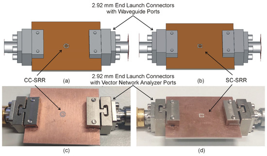
Figure 9.
(a) Simulated model of optimized CC-SRR sensor with end launch connectors, (b) Simulated model of optimized SC-SRR sensor with end launch connectors, (c) Fabricated CC-SRR sensor with end launch connectors, and (d) Fabricated SC-SRR sensor with end launch connectors.
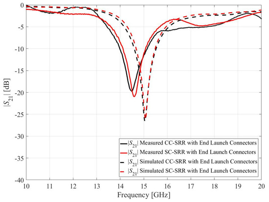
Figure 10.
Measured and simulated transmission coefficients (S21) of the optimized sensors with end launch connectors.
5. Calibration Procedure and Results
A three-dimensional dielectric container (internal size = 5 mm × 5 mm × 1 mm) is incorporated into the design for the positioning of the sample under test (SUT), which enables precision and accuracy for the measurement operations, as illustrated in Figure 11. A polylactide acid (PLA) container is manufactured using a 3D printer owing to the PLA properties of excellent surface quality, decent strength, and low sensitivity to temperature variations. The PLA container is attached to the SC-SRR sensor in the ground plane using cyanoacrylate adhesive, as shown in Figure 11a. To calibrate the sensor, five SUTs with known relative permittivity values, namely TLY-5 (εr = 2.2), AD250C (εr = 2.5), RO4003C (εr = 3.38), RF-35 (εr = 3.5), and FR4 (εr = 4.3), and fixed dimensions of 5 mm × 5 mm × 1 mm, are placed inside the PLA container, as shown in Figure 11b. The values of the permittivity used for calibration are obtained from the datasheets provided by the manufacturer of these SUT. According to the materials’ datasheet, the uncertainty in permittivity values is +/−0.05. A 1-mm-thick sample is used to eliminate the ambient effect because the impact of the SUT’s thickness begins to diminish after 1 mm (cf. Figure 6). The transmission responses of the sensor loaded with the aforementioned SUTs are measured ten times for each material to minimize stochastic errors. Table 3 shows the obtained results, i.e., the mean and standard deviation of the loaded sensor resonant frequencies. A variety of variables can influence the variation between calibration runs for the same dielectric material. The first is the air gap between the sample and the resonator, the second is the sample condition, and the third is the surrounding environment, such as air humidity or temperature, of the measuring setup. Table 3 illustrates a significant standard deviation in the measured resonance frequency among all ten runs. The frequency shift appears to saturate with larger dielectric constants. The resonant frequency is nearly identical at larger relative dielectric constants (particularly for RF35 and FR4). This indicates that the sensor has a low dynamic range despite its high sensitivity. Instead of a dynamic range, a resonator with extremely high sensitivity is required to evaluate oils with relative permittivity values ranging from 2.22 to 3.08. The data in Table 3 are employed to establish an inverse regression model that permits the direct identification of the unknown permittivity of the SUT, based on the measured resonant frequency f0.
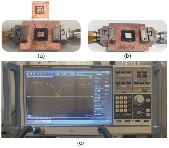
Figure 11.
Photographs of the SC-SRR sensor’s fabricated prototype: (a) bottom view with PLA container and the optimized CSRR, (b) sensor with MUT, and (c) Vector network analyzer (VNA) while measuring the unloaded sensor.
Table 3.
Measurement results for the calibration materials.
The model is assumed to have the following analytical form [38]:
Here, εr stands for the relative permittivity of the SUT. This particular analytical form is chosen based on the initial analysis of the dependence between the observed resonant frequency and dielectric permittivity of the material. The objective is to employ a simple form parameterized using a small number of coefficients (here, three). On the one hand, this allows for accounting for the weak nonlinearity of the aforementioned relationship. On the other hand, it allows us to maintain the uniqueness of the solution to the regression task, and to smoothen out fluctuations due to measurement errors. The model is parameterized using a = [a0 a1 a2]T. This vector is identified by solving the regression tasks εr.j = F(f0.j,a), j = 1, …, 5, with εr.j and f0.j being the dielectric permittivity and measured sensor resonant frequency as shown in Table 3. The least-square solution to the above regression problems is equivalent to minimizing E(a), defined as:
The minimum can be found analytically as:
where the kth row of the matrix A is [1 f0.k f0.k2], k = 1, …, 5.
Upon substituting the data in Table 3, we find a = [58.697 −7.207 0.223]T, i.e., the regression model takes the form of
Figure 12 shows the plot of the calibration model along with the error bars corresponding to the standard deviations of the measurement data (cf. Table 3). Based on these, it can be estimated that the sensor measurement error, when using the calibration model, is less than five percent. Five oils with known dielectric characteristics are used to validate the inverse regression model; the extracted oil permittivity values are remarkably similar to those reported in the literature.
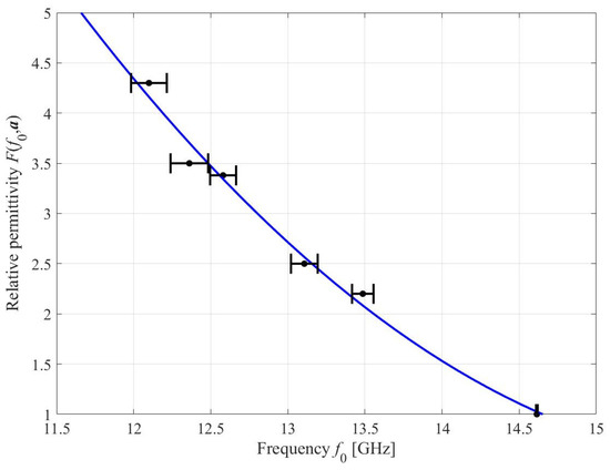
Figure 12.
Calibration model of the proposed sensor. Circles correspond to the MUT measurement data in Table 3. Horizontal bars represent standard deviations of the measurement data.
6. Application Case Study: Oil Measurement
The calibration model is used to evaluate the relative permittivity of commonly available oils such as diesel oil (εr = 2.2) [39], sunflower oil (εr = 2.44) [40], mustard oil (εr = 2.70) [41], almond oil (εr = 3.03) [42], and olive oil (εr = 3.08) [42]. For this purpose, 25 μL of each oil was poured into the PLA container as shown in Figure 13. A single-channel adjustable volume pipette is used to control the volume of the oil samples, as shown in Figure 12c. In order to avoid contamination by the previous oil sample, the PLA container is cleaned with alcohol each time, and the alcohol is left to evaporate so that the resonant frequency of the unloaded sensor is not compromised. The sensor’s transmission response due to interaction with the oils was measured and plotted as shown in Figure 14. The resonant frequencies of the optimized sensor due to interaction with diesel engine oil, sunflower oil, mustard oil, almond oil, and olive oil are 13.39 GHz, 13.17 GHz, 12.94 GHz, 12.84 GHz, and 12.76 GHz, respectively. The corresponding relative permittivity of these oils obtained from the calibration model is 2.2, 2.48, 2.80, 2.97, and 3.06, which are close to the values available in the literature.
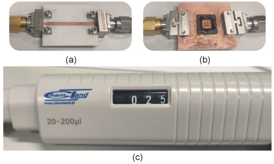
Figure 13.
Measurement setup: (a) top view of the sensor, (b) bottom view with PLA container and oil under test, and (c) single-channel adjustable volume pipette used for volume control of the oils.
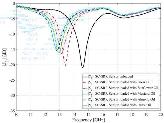
Figure 14.
Calibration model of the proposed sensor. Circles correspond to the MUT measurement data in Table 3. Horizontal bars represent the standard deviations of the measurement data.
To compare the performance of the manufactured sensor to that of other sensors, the most important criterion is relative sensitivity. The relative sensitivity of the optimized sensor can be calculated using the following relation [43]:
where fu is the sensor’s resonant frequency without SUT and fl is the resonant frequency while interacting with the SUT of relative permittivity εr.
The optimized sensor provides a minimum frequency shift of 1.23 GHz and a maximum sensitivity of 7.01 percent due to interaction with the diesel oil. According to (10), the sensitivity is directly proportional to the resonant frequency of the sensor. While the resonant frequency is inversely proportional to the permittivity of the substrate. As a result, if we use a different substrate with high relative permittivity, such as FR4 (εr = 4.3), the resonant frequency of the same sensor will decrease, resulting in a decrease in sensor sensitivity. Table 4 compares the relative sensitivity of the sensor proposed in this work and the state-of-the-art sensors reported in the literature. It can be observed that the proposed device clearly outperforms the benchmark in terms of relative sensitivity.
Table 4.
Comparative analysis of contemporary sensors based on optimization, calibration method, and relative sensitivity.
7. Conclusions
This article presented an optimization and inverse-model-based calibration technique for circular complementary split ring resonators (CC-SRR) and square complementary split ring resonators (SC-SRR) linked to microstrip transmission lines. The CC-SRR and SC-SRR are described using five independent parameters and these variables are meticulously tuned to allocate the resonant frequency of the sensors at 15 GHz. Each sensor is subject to sensitivity analysis by altering the permittivity, permeability, dielectric, and magnetic loss tangents of the sample under test after obtaining the equivalent transmission response using the optimization technique. This approach cannot be generalized to lossy properties or non-unitary magnetic permeability values because practical materials are categorized according to their dielectric constant. The effect of 2.92 mm end launch connectors on the transmission responses of unloaded optimized sensors is numerically calculated, revealing that they have a maximum effect of 0.03 GHz on the resonance frequencies, despite the fact that the simulation takes five times longer than with sensors without end launch connectors. Fabrication tolerance is a crucial component that causes the simulation and measurement to disagree. The fabrication tolerance of the CC-SRR and SC-SRR is investigated by comparing the unloaded sensors’ simulated and measured transmission coefficients. The discrepancy between the simulated and measured resonance frequencies is 3.65 percent for the CC-SRR sensor and 3.03 percent for the SC-SRR sensor. The fabricated sensor based on SC-SRR is calibrated through measurements of dielectric samples of known permittivity and the inverse regression model. For the positioning of the sample under test, a three-dimensional dielectric container is incorporated into the design, providing precision and reliability for the measurement procedures. Application case studies carried out for several oil samples demonstrate competitive sensitivity of 7.01 percent for the optimized sensor, outperforming the state-of-the-art sensors reported in the literature.
Author Contributions
T.H. contributed to the design, simulation, evaluation, characterization, and implementation of the proposed sensors. In addition, they participated in the execution of experiments, the collection of data, the cataloging of references, and the overall composition of the manuscript. S.K. contributed to the conception, direction, funding, and critical review of the article for significant intellectual approval. They also contributed to the revision of the paper and proposed the design optimization method and the inverse regression model. All authors have read and agreed to the published version of the manuscript.
Funding
This work was supported in part by the Icelandic Centre for Research (RANNIS) under Grant 217771 and in part by the National Science Centre of Poland under Grant 2018/31/B/ST7/02369.
Institutional Review Board Statement
Not applicable.
Informed Consent Statement
Not applicable.
Data Availability Statement
Not applicable.
Conflicts of Interest
The authors declare no conflict of interest.
References
- Islam, M.R.; Islam, M.T.; Salaheldeen, M.; Bais, B.; Almalki, H.A.; Alsaif, H.; Islam, M.S. Metamaterial sensor based on rectangular enclosed adjacent triple circle split ring resonator with good quality factor for microwave sensing application. Sci. Rep. 2022, 12, 6792. [Google Scholar] [CrossRef] [PubMed]
- Iyer, A.K.; Eleftheriades, G.V. Negative refractive index metamaterials supporting 2-D waves. In Proceedings of the 2002 IEEE MTT-S International Microwave Symposium Digest, Seattle, WA, USA, 2–7 June 2002; Volume 2, pp. 1067–1070. [Google Scholar] [CrossRef]
- Oliner, A. A planar negative-refractive-index medium without resonant elements. In Proceedings of the IEEE MTT-S International Microwave Symposium Digest, Philadelphia, PA, USA, 8–13 June 2003; Volume 1, pp. 191–194. [Google Scholar] [CrossRef]
- Caloz, Z.; Itoh, T. Transmission line approach of left-handed (LH) materials and microstrip implementation of an artificial LH transmission line. IEEE Trans. Antennas Propag. 2004, 52, 1159–1166. [Google Scholar] [CrossRef]
- Mohammadi, S.; Adhikari, K.K.; Jain, M.C.; Zarifi, M.H. High-resolution, sensitivity-enhanced active resonator sensor using substrate-embedded channel for characterizing low-concentration liquid mixtures. IEEE Trans. Microw. Theory Tech. 2022, 70, 576–586. [Google Scholar] [CrossRef]
- Mayani, M.G.; Herraiz-Martínez, F.J.; Jain, M.C.; Domingo, J.M.; Giannetti, R. Resonator-based microwave metamaterial sensors for instrumentation: Survey, classification, and performance comparison. IEEE Trans. Instrum. Meas. 2021, 70, 9503414. [Google Scholar] [CrossRef]
- Pendry, J.B.; Holden, A.J.; Robbins, D.J.; Stewart, W.J. Magnetism from conductors and enhanced nonlinear phenomena. IEEE Trans. Microw. Theory Tech. 1999, 47, 2075–2084. [Google Scholar] [CrossRef]
- Falcone, F.; Lopetegi, T.; Baena, J.D.; Marqués, F.; Sorolla, M. Effective negative epsilon stopband microstrip lines based on complementary split ring resonators. IEEE Microw. Wirel. Compon. Lett. 2004, 14, 280–282. [Google Scholar] [CrossRef]
- Baena, J.D.; Bonache, J.; Martín, F.; Sillero, R.M.; Falcone, F.; Lopetegi, T.; Laso, M.A.G.; García, J.; Gil, I.; Portillo, M.F.; et al. Equivalent-circuit models for split-ring resonators and complementary split-ring resonators coupled to planar transmission lines. IEEE Trans. Microw. Theory Tech. 2005, 53, 1451–1461. [Google Scholar] [CrossRef]
- Vélez, A.; Bonache, J.; Martín, F. Varactor-loaded complementary split ring resonators (vlcsrr) and their application to tunable metamaterial transmission lines. IEEE Microw. Wirel. Compon. Lett. 2008, 18, 28–30. [Google Scholar] [CrossRef]
- Hou, R.; Ren, J.; Zuo, M.; Yin, Y.Z. Magnetoelectric dipole filtering antenna based on CSRR with third harmonic suppression. IEEE Antennas Wirel. Propag. Lett. 2021, 20, 1337–1341. [Google Scholar] [CrossRef]
- Haq, T.; Khan, M.F.; Siddiqui, O.F. Design and implementation of waveguide bandpass filter using complementary metaresonator. Appl. Phys. A. 2016, 34, 34. [Google Scholar] [CrossRef]
- Dong, Y.D.; Yang, T.; Itoh, T. Substrate Integrated Waveguide Loaded by Complementary Split-Ring Resonators and Its Applications to Miniaturized Waveguide Filters. IEEE Trans. Microw. Theory Tech. 2009, 57, 2211–2223. [Google Scholar] [CrossRef]
- Alahnomi, R.A.; Zakaria, Z.; Yussof, Z.M.; Althuwayb, A.A.; Alhegazi, A.; Alsariera, H.; Rahman, A. Review of recent microwave planar resonator based sensors: Techniques of complex permittivity extraction, applications, open challenges and future research directions. Sensors 2021, 21, 2267. [Google Scholar] [CrossRef]
- Rawat, V.; Kitture, R.; Kumari, D.; Rajesh, H.; Banerjee, S.; Kale, S.N. Hazardous materials sensing: An electrical metamaterial approach. J. Magnetism Magn. Mater. 2016, 415, 77–81. [Google Scholar] [CrossRef]
- Chuma, E.L.; Iano, Y.; Fontgalland, G.; Roger, L.L.B. Microwave sensor for liquid dielectric characterization based on metamaterial complementary split ring resonator. IEEE Sens. J. 2018, 18, 9978–9983. [Google Scholar] [CrossRef]
- Boybay, M.S.; Ramahi, O.M. Non-destructive thickness measurement using quasi-static resonators. IEEE Microw. Wirel. Compon. Lett. 2013, 23, 217–219. [Google Scholar] [CrossRef]
- Salim, A.; Lim, S. Complementary split ring resonator loaded microfluidic ethanol chemical sensor. Sensors 2016, 16, 1802. [Google Scholar] [CrossRef]
- Lee, C.S.; Yang, C.L. Thickness and permittivity measurement in multi layered dielectric structures using complementary split ring resonator. IEEE Sens. J. 2014, 14, 695–700. [Google Scholar] [CrossRef]
- Ebrahimi, A.; Withayachumnankul, W.; Al-Sarawi, S.; Abbott, D. High sensitivity metamaterial inspired sensor for microfluidic dielectric characterization. IEEE Sens. J. 2014, 14, 1345–1351. [Google Scholar] [CrossRef]
- Lee, C.S.; Yang, C.L. Single compound complementary split ring resonator for simultaneously measuring the permittivity and thickness of dual layer dielectric materials. IEEE Trans. Microw. Theory Tech. 2015, 63, 2010–2023. [Google Scholar] [CrossRef]
- Jang, C.; Park, J.K.; Lee, H.J.; Yun, G.H.; Yook, J.G. Non-invasive fluidic glucose detection based on dual microwave complementary split ring resonators with a switching circuit for environmental effect elimination. IEEE Sens. J. 2020, 20, 8520–8527. [Google Scholar] [CrossRef]
- Zhang, X.; Ruan, C.J.; Wang, W.; Cao, Y. Submersible high sensitivity microwave sensor for edible oil detection and quality analysis. IEEE Sens. J. 2021, 21, 13230–13238. [Google Scholar] [CrossRef]
- Tiwari, N.K.; Singh, S.P.; Akhtar, M.J. Novel improved sensitivity planar microwave probe for adulteration detection in edible oils. IEEE Microw. Wirel. Compon. Lett. 2019, 29, 164–166. [Google Scholar] [CrossRef]
- Haq, T.; Ruan, C.J.; Zhang, X.; Kosar, A.; Ullah, S. Low cost and compact wideband microwave notch filter based on miniaturized complementary metaresonator. Appl. Phys. A. 2019, 125, 662. [Google Scholar] [CrossRef]
- Ansari, M.A.H.; Jha, A.K.; Akhter, Z.; Akhtar, M.J. Multi-Band RF Planar Sensor Using Complementary Split Ring Resonator for Testing of Dielectric Materials. IEEE Sens. J. 2018, 18, 6596–6606. [Google Scholar] [CrossRef]
- Javed, A.; Arif, A.; Zubair, M.; Mehmood, M.Q.; Riaz, K. A low-cost multiple complementary split-ring resonator-based microwave sensor for contactless dielectric characterization of liquids. IEEE Sens. J. 2020, 20, 11326–11334. [Google Scholar] [CrossRef]
- Jiang, Q.; Yu, Y.; Zhao, Y.; Zhang, Y.; Liu, L.; Li, Z. Ultra compact effective localized surface plasmonic sensor for permittivity measurement of aqueous ethanol solution with high sensitivity. IEEE Trans. Instrum. Meas. 2021, 70, 6008709. [Google Scholar] [CrossRef]
- Parvathi, S.L.; Gupta, R. Two channel dual band microwave EBG sensor for simultaneous dielectric detection of liquids. Int. J. Electron. Commun. 2022, 146, 154099. [Google Scholar] [CrossRef]
- Armghan, A.; Alanazi, T.M.; Altaf, A.; Haq, T. Characterization of dielectric substrates using dual band microwave sensor. IEEE Access 2021, 9, 62779–62787. [Google Scholar] [CrossRef]
- Cao, Y.; Ruan, C.J.; Chen, K.; Zhang, X. Research on a high-sensitivity asymmetric metamaterial structure and its application as microwave sensor. Sci. Rep. 2022, 12, 1255. [Google Scholar] [CrossRef]
- Qureshi, S.A.; Abidin, Z.Z.; Ashyap, A.; Majid, H.A.; Kamarudin, M.R.; Yue, M.; Zulkipli, M.S.; Nebhen, J. Millimetre wave metamaterial based sensor for characterization of cooking oils. Int. J. Antennas Propag. 2021, 10, 5520268. [Google Scholar] [CrossRef]
- Akgol, O.; Unal, E.; Bagmanci, M.; Karaaslan, M.; Sevim, U.K.; Ozturk, M.; Bhadauria, A. A nondestructive method for determining fiber content and fiber ratio in concentrates using a metamaterial sensor based on a V shaped resonator. J. Electron. Matter. 2019, 48, 2469–2481. [Google Scholar] [CrossRef]
- Haq, T.; Ruan, C.J.; Zhang, X.; Ullah, S. Complementary metamaterial sensor for nondestructive evaluation of dielectric substrates. Sensors 2019, 19, 2100. [Google Scholar] [CrossRef]
- Conn, A.R.; Gould, N.I.M.; Toint, P.L. Trust Region Methods; MPS-SIAM Series on Optimization; SIAM Digital Library: Philadelphia, PA, USA, 2000. [Google Scholar]
- Koziel, S.; Pietrenko-Dabrowska, A. Expedited optimization of antenna input characteristics with adaptive Broyden updates. Eng. Comput. 2019, 37, 3. [Google Scholar] [CrossRef]
- Haq, T.; Ruan, C.J.; Ullah, S.; Kosar, A. Dual notch microwave sensors based on complementary metamaterial resonators. IEEE Access 2019, 7, 153489–153498. [Google Scholar] [CrossRef]
- Haq, T.; Koziel, S. Inverse Modeling and Optimization of CSRR-Based Microwave Sensors for Industrial Applications. IEEE Trans. Microw. Theory Tech. 2022, 70, 4796–4804. [Google Scholar] [CrossRef]
- DeSouza, J.D.; Scherer, M.D.; Cáceres, C.A.S.; Caires, A.R.L.; M’Peko, J.C.A. A close dielectric spectroscopic analysis of diesel/biodiesel blends and potential dielectric approaches for biodiesel content assessment. Fuel 2013, 105, 705–710. [Google Scholar] [CrossRef]
- Zhang, X.; Ruan, C.J.; Cao, Y. A dual-mode microwave sensor for edible oil characterization using magnetic-LC Resonators. Sens. Actuators A Phys. 2022, 333, 113275. [Google Scholar] [CrossRef]
- Kumar, A.V.P.; Goel, A.; Kumar, R.; Ojha, A.K.; John, J.K.; Joy, J. Dielectric characterization of common edible oils in the higher microwave frequencies using cavity perturbation. J. Microw. Power Electromagn. Energy 2019, 53, 48–56. [Google Scholar] [CrossRef]
- Mathew, T.; Vyas, A.D.; Tripathi, D. Dielectric properties of some edible and medicinal oils at microwave frequency. Canadian J. Pure Appl. Sci. 2009, 3, 953–957. [Google Scholar]
- Lee, C.S.; Bai, B.; Song, Q.R.; Wang, Z.Q.; Li, G.F. Open complementary split ring resonator sensor for dropping based liquid dielectric characterization. IEEE Sens. J. 2019, 19, 11880–11890. [Google Scholar] [CrossRef]
- Rowe, D.J.; Malki, S.; Abduljabar, A.A.; Porch, A.; Barrow, D.A.; Allender, C.J. Improved split ring resonator for microfluidic sensing. IEEE Trans. Microw. Theory Tech. 2014, 62, 689–699. [Google Scholar] [CrossRef]
- Ebrahimi, A.; Scott, J.; Ghorbani, K. Ultrahigh sensitivity microwave sensor for microfluidic complex permittivity measurement. IEEE Trans. Microw. Theory Tech. 2019, 67, 4269–4277. [Google Scholar] [CrossRef]
- Alahnomi, R.A.; Zakaria, Z.; Ruslan, E.; Ab Rashid, S.R.; Mohd Bahar, A.A. High Q sensor based on symmetrical split ring resonator with spurlines for solid material detection. IEEE Sens. J. 2017, 17, 2766–2775. [Google Scholar] [CrossRef]
- Romera, G.G.; Herraiz-Martinez, M.J.; Gil, M.; Martinez-Martinez, J.J.; Segovia-Vargas, D. Submersible printed split ring resonator based sensor for thin film detection and permittivity characterization. IEEE Sens. J. 2016, 16, 3587–3596. [Google Scholar] [CrossRef]
- Su, L.; Mata-Contreras, J.; Velez, P.; Fernandez-Prieto, A.; Martin, F. Analytical method to estimate the complex permittivity of oil samples. Sensors 2016, 18, 984. [Google Scholar] [CrossRef]
- Alotaibi, S.A.; Cui, Y.; Tentzeris, M.M. CSRR Based Sensors for Relative Permittivity Measurement with Improved and Uniform Sensitivity Throughout [0.9–10.9] GHz Band. IEEE Sens. J. 2020, 20, 4667–4678. [Google Scholar] [CrossRef]
- Hao, H.; Wang, D.; Wang, Z.; Yin, B.; Ruan, W. Design of a High Sensitivity Microwave Sensor for Liquid Dielectric Constant Measurement. Sensors 2020, 20, 5598. [Google Scholar] [CrossRef]
- Armghan, A. Complementary metaresonator sensor with dual notch resonance for evaluation of vegetable oils in C and X bands. Appl. Sci. 2021, 11, 5734. [Google Scholar] [CrossRef]
- Haq, T.; Ruan, C.J.; Zhang, X.; Ullah, S.; Fahad, A.K.; He, W. Extremely sensitive microwave sensor for evaluation of dielectric characteristics of low permittivity materials. Sensors 2020, 20, 1916. [Google Scholar] [CrossRef]
- Zheng, H.X. Measurements of complex permittivity using dielectric resonator at 60 GHz. In Proceedings of the 2006 7th International Symposium on Antennas, Propagation & EM Theory, Guilin, China, 26–29 October 2006. [Google Scholar] [CrossRef]
- Omer, A.E.; Shaker, G.; Safavi-Naeini, S.; Ngo, K.; Shubair, R.M.; Alquie, G.; Deshours, F.; Kokabi, H. Multiple-cell microfluidic dielectric resonator for liquid sensing applications. IEEE Sens. J. 2021, 5, 6094–6104. [Google Scholar] [CrossRef]
- Mayani, M.G.; Herraiz-Martinez, F.J.; Domingo, J.M.; Giannetti, R.; Garia, C.R.M. A novel dielectric resonator-based passive sensor for drop-volume binary mixtures classification. IEEE Sens. J. 2021, 18, 20156–20165. [Google Scholar] [CrossRef]
Disclaimer/Publisher’s Note: The statements, opinions and data contained in all publications are solely those of the individual author(s) and contributor(s) and not of MDPI and/or the editor(s). MDPI and/or the editor(s) disclaim responsibility for any injury to people or property resulting from any ideas, methods, instructions or products referred to in the content. |
© 2023 by the authors. Licensee MDPI, Basel, Switzerland. This article is an open access article distributed under the terms and conditions of the Creative Commons Attribution (CC BY) license (https://creativecommons.org/licenses/by/4.0/).