


Applications of Computer Vision-Based Structural Monitoring on Long-Span Bridges in Turkey


Abstract
:1. Introduction
1.1. Statement of the Problem
1.2. Objectives and Scope
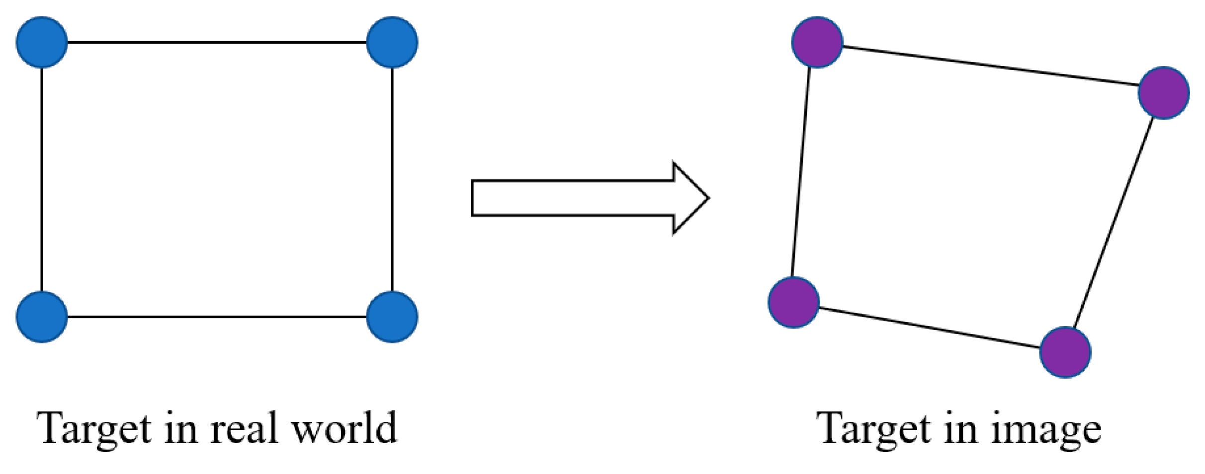
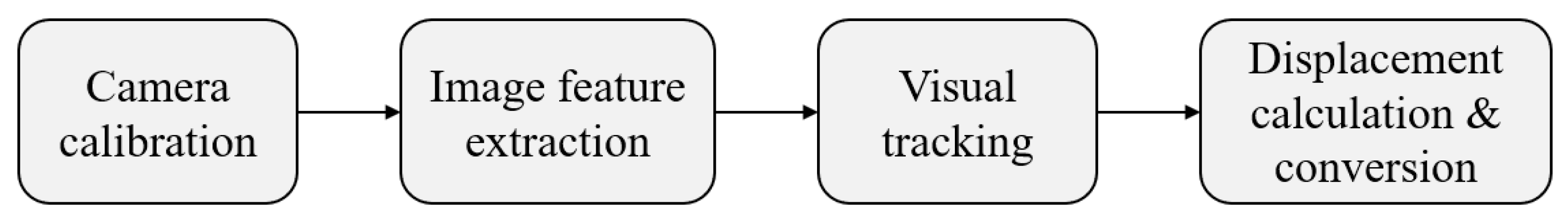
2. Computer Vision-Based Displacement Measurement Using Zero-Mean Normalized Cross-Correlation and Homography Transformation
3. Experiment on the First Bosphorus Bridge
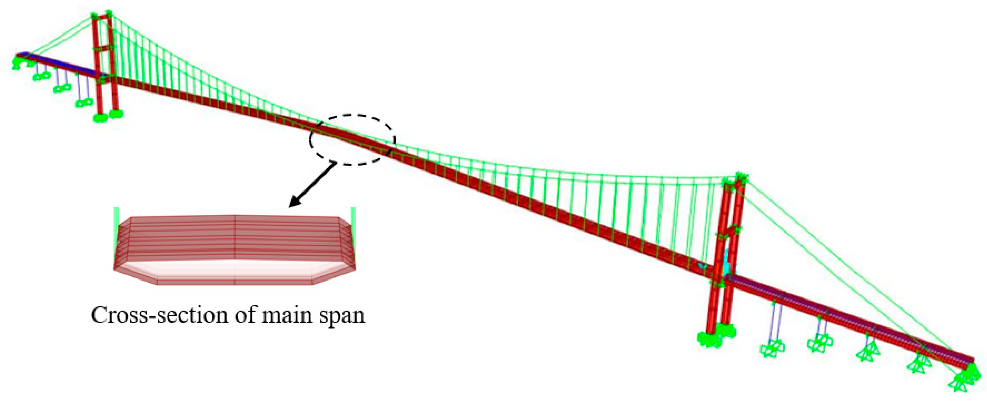
3.1. General Features of the First Bosphorus Bridge
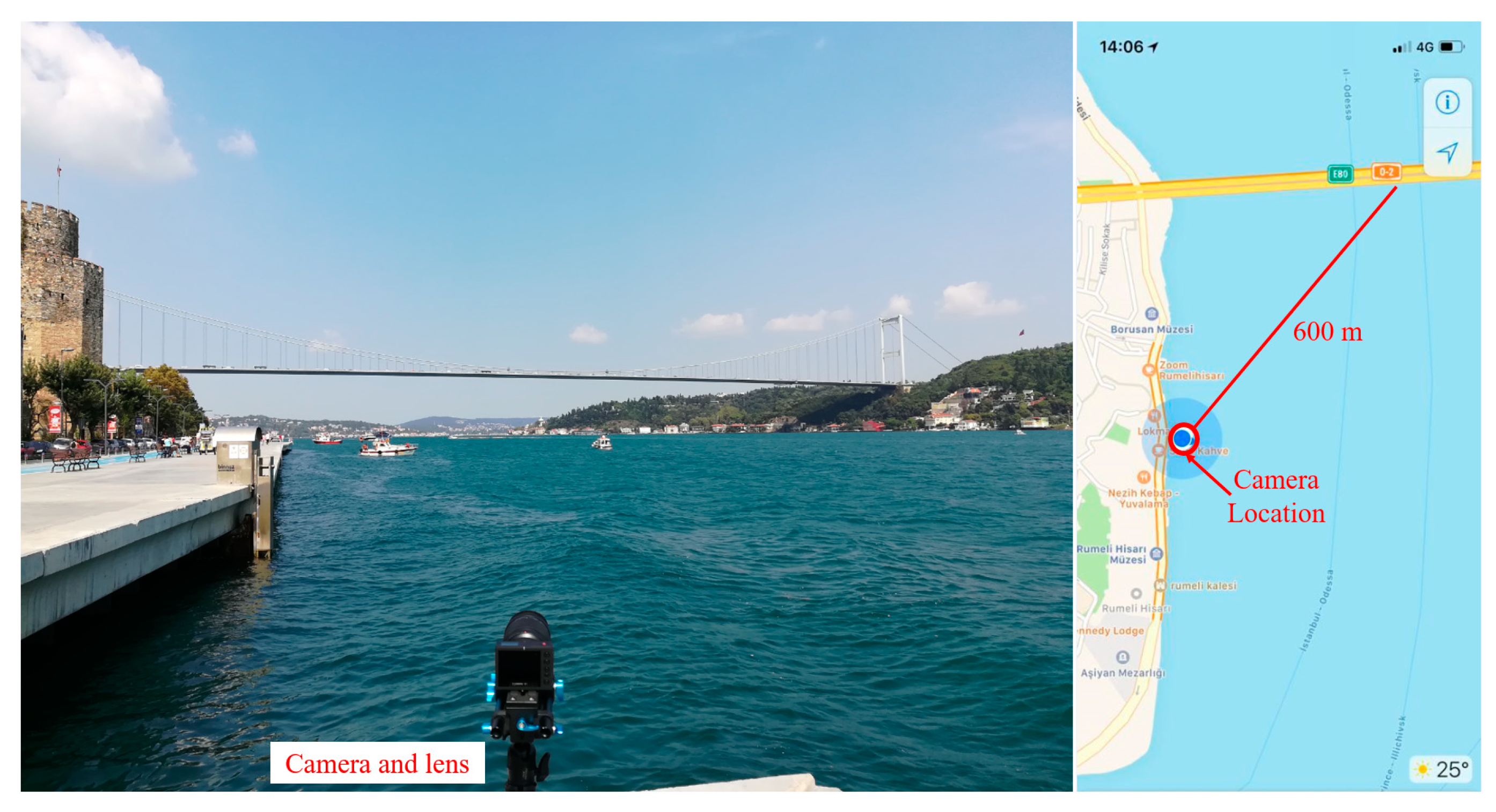
3.2. Experimental Setup
3.3. Results Analysis and Verification
4. Experiment on the Second Bosphorus Bridge
4.1. General Features of the Second Bosphorus Bridge
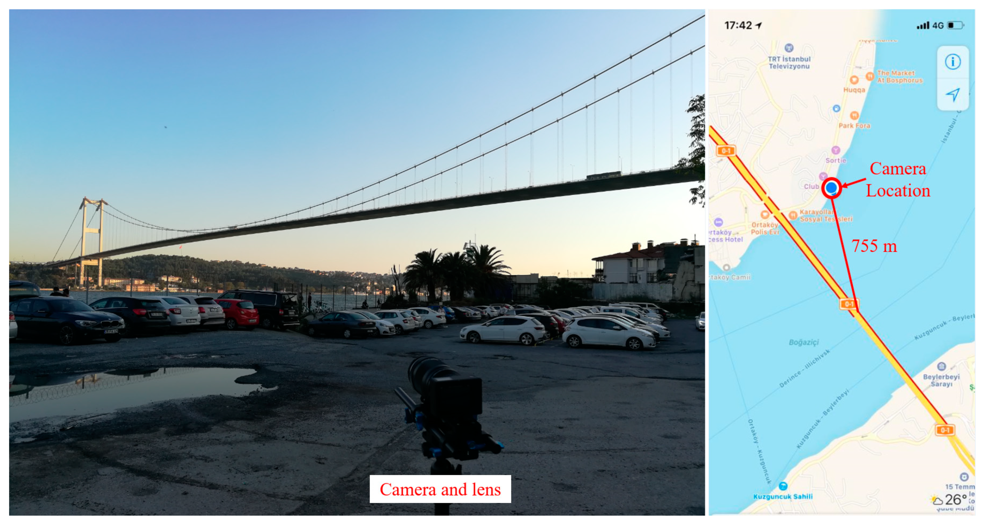
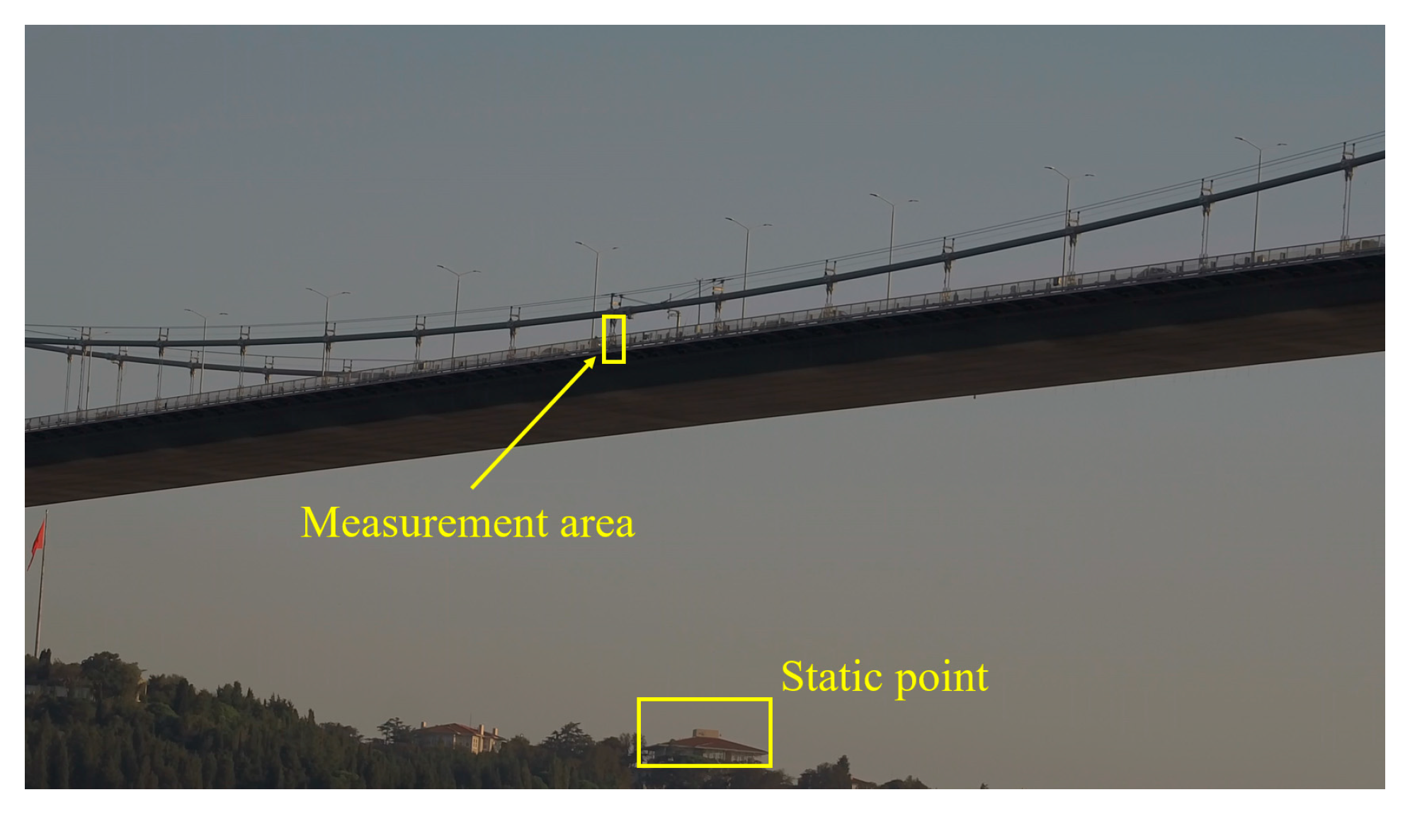
4.2. Experimental Setup
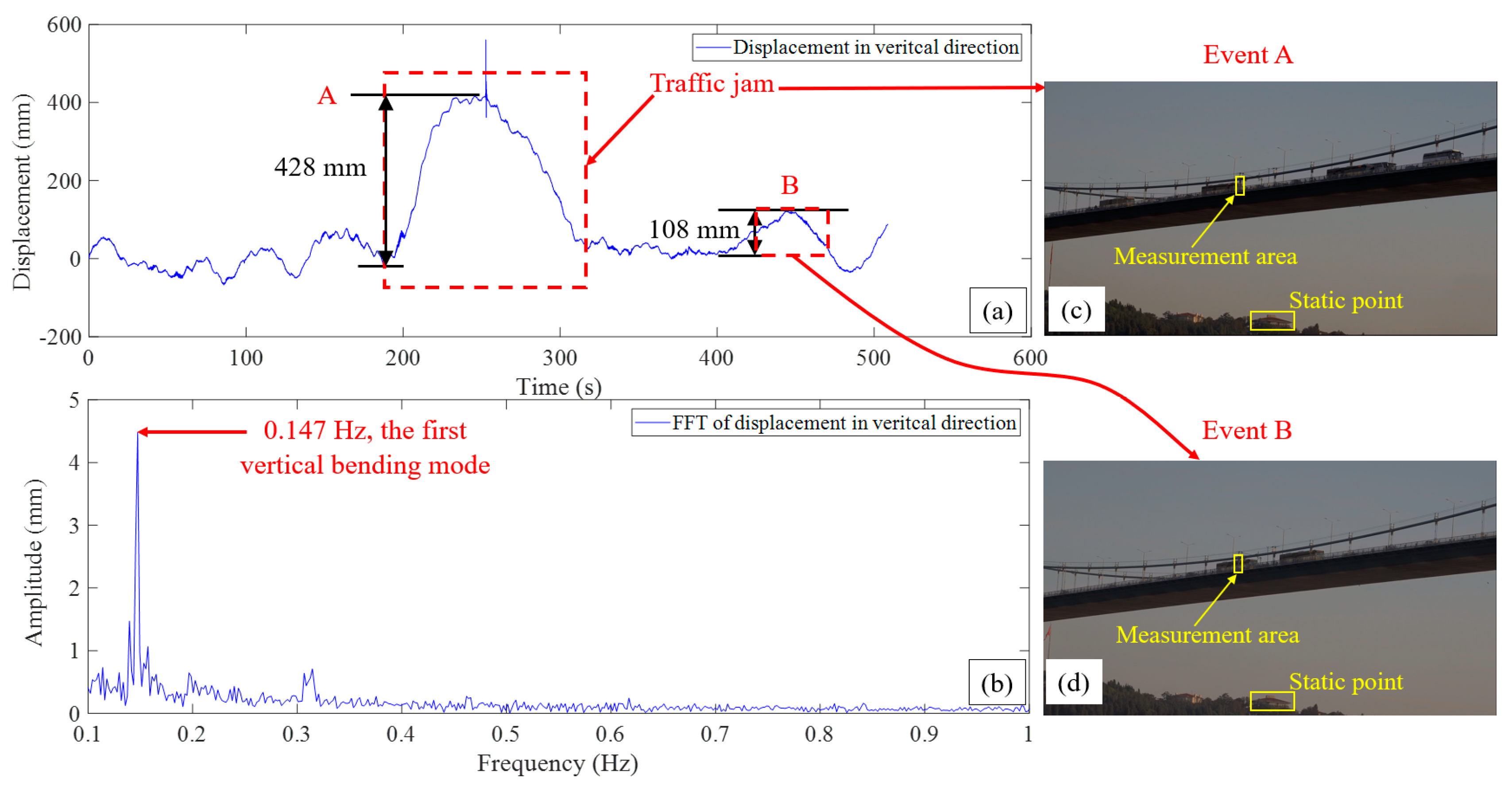
4.3. Results Analysis and Verification
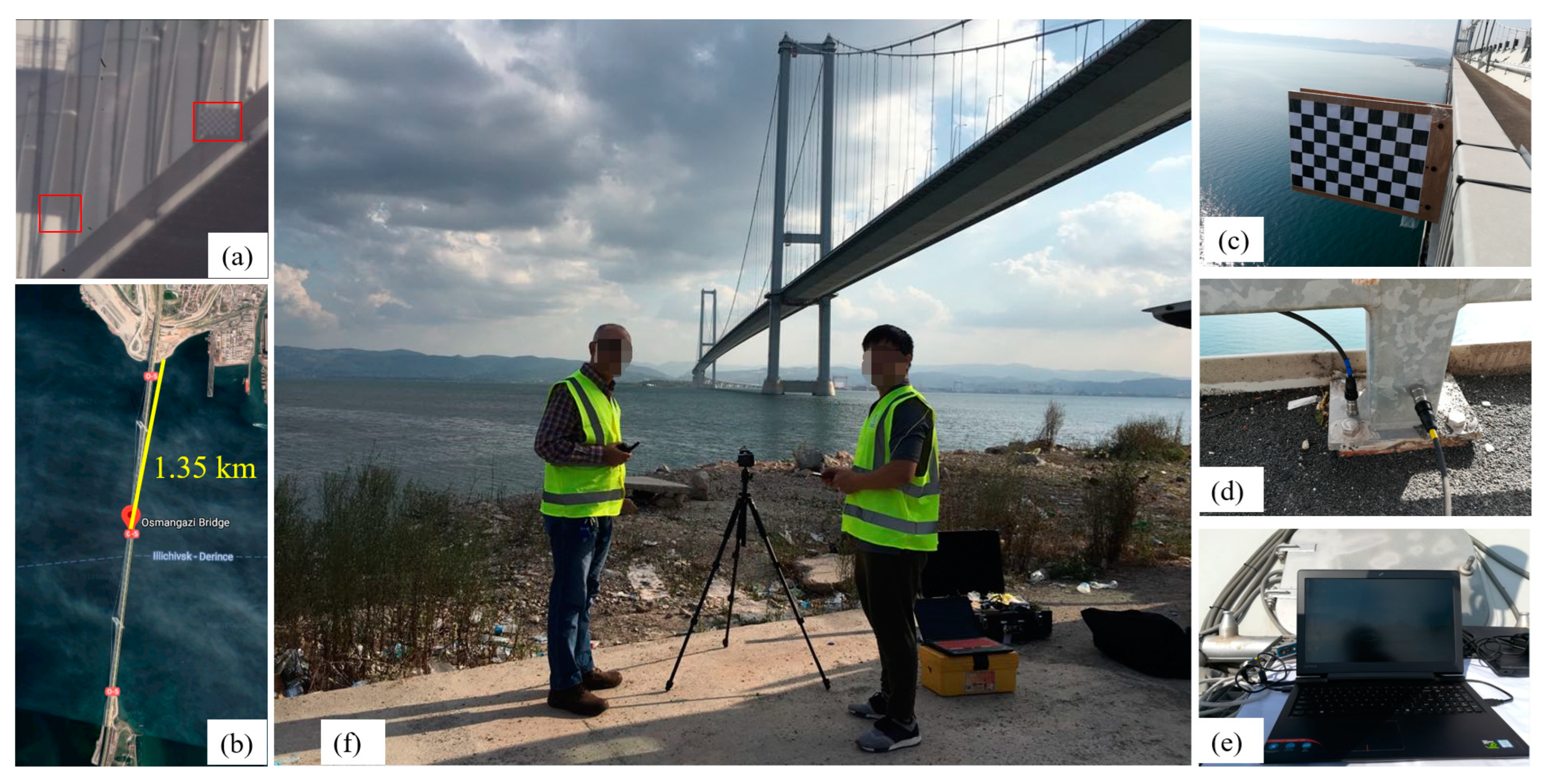
5. Experiment on the Osman Gazi Bridge
5.1. General Features of the Osman Gazi Bridge
5.2. First Experiment
5.2.1. Experimental Setup
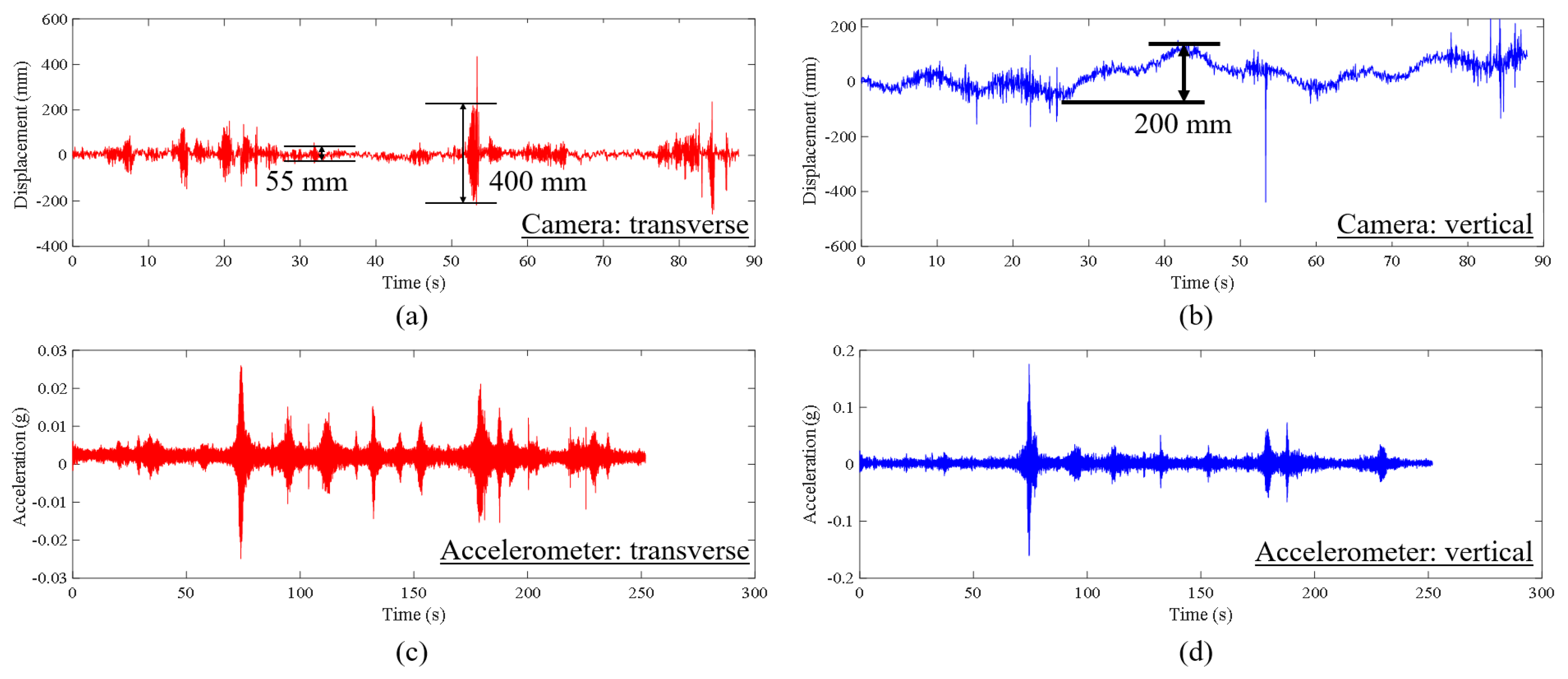
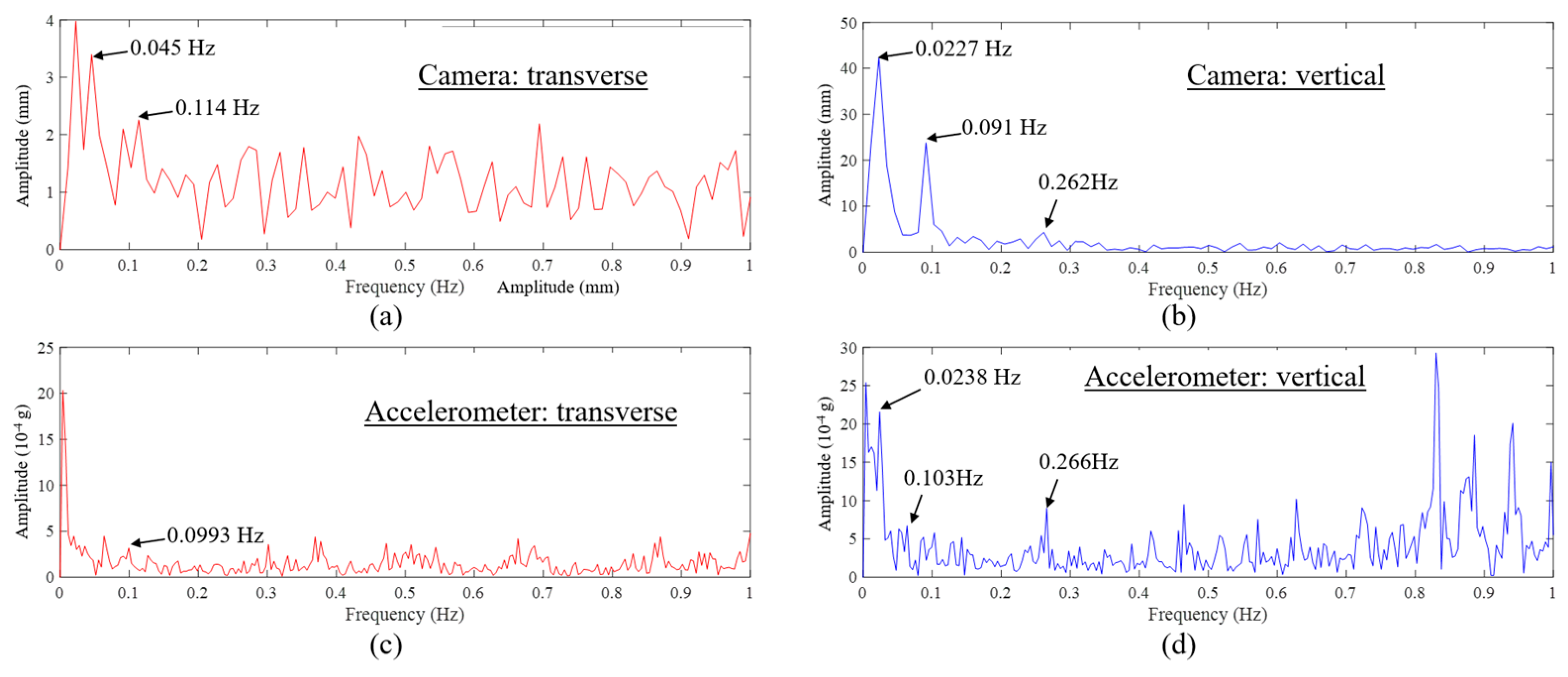
5.2.2. Results Analysis and Verification
5.3. Second Experiment
5.3.1. Experimental Setup
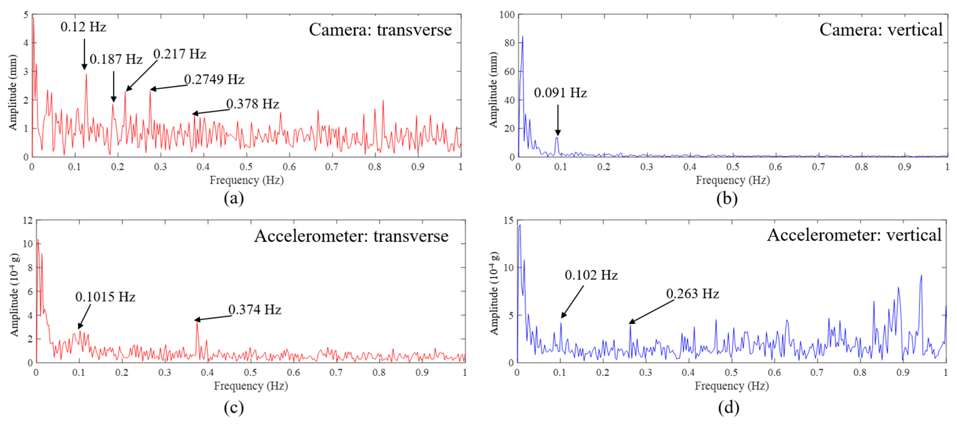
5.3.2. Result Analysis and Verification
6. Discussion and Considerations
- (1)
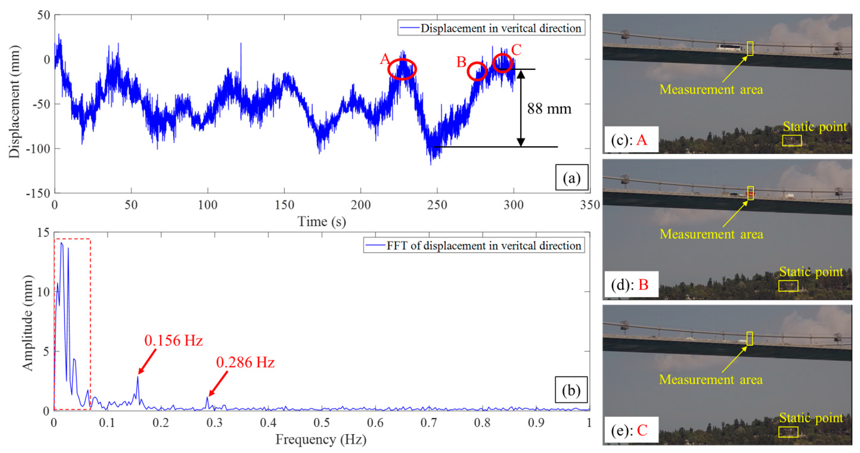
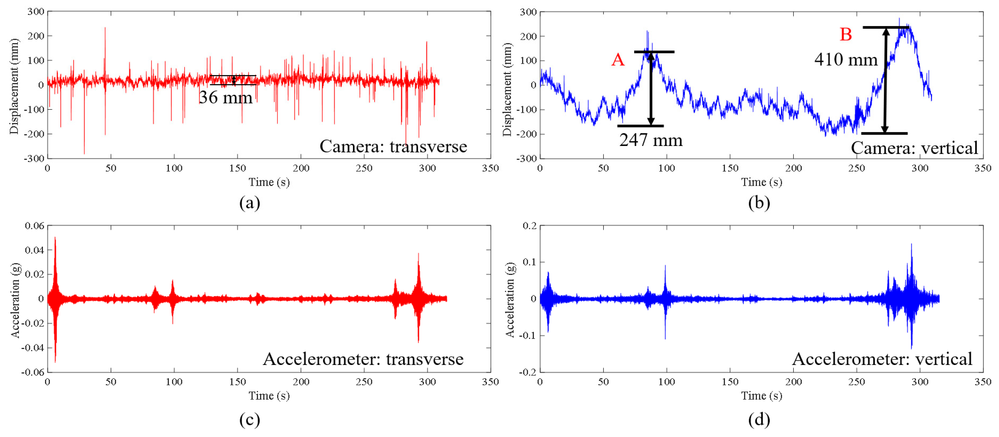
- Considerations of the verification approaches: Continuously measuring the structural displacement of large civil structures, particularly long-span bridges crossing rivers, channels, and seas, is a challenging task. Therefore, verifying computer vision-based structural monitoring can be difficult, especially when there is no access to other types of sensors that can directly measure displacement. In this study, verification was conducted using the following two approaches: (a) verifying the monitoring results in the frequency domain using data from both accelerometers and FE models, and (b) verifying displacement magnitude results by estimating a potential range with 3D FE models and observing traffic conditions from images recorded by the camera during displacement measurement experiments. The comparisons yield closely aligned results, providing encouraging evidence to support the use of computer vision-based monitoring from long distances for applications such as long-span bridges.
- (2)
- Overview of the results: Displacement and frequency differences between computer vision and FEM results are about 5% and 2%, respectively, for the First Bosphorus Bridge where the camera location is 600 m from the bridge. For the Second Bosphorus Bridge dynamic, the camera distance is 755 m and the difference of sensor and camera-based dynamic results is about 3%. As for the Osman Gazi Bridge, the camera location is 1350 m, and here, we obtain differences for sensor and camera-based frequencies in the order of 1.5% to 18%. The long distance of measurement, possible vibration of the target chess board and camera vibrations, although minimized as much as possible, may explain the relatively high transversal vibration difference. It should also be noted that another camera-based monitoring conducted at Osman Gazi from a 750 m distance showed good consistency with the 1350 m monitoring results.
- (3)
- Challenges in practice: The application of computer vision-based monitoring to long-span bridges presents certain challenges due to adverse environmental factors such as airflow uncertainties, camera shaking problems due to wind effects or ground motion, and anomalous light changes, which can result in lower measurement accuracy compared to laboratory experiments and close-range measurements. This issue is particularly pronounced when using extended zoom lenses or lenses with large focal lengths, which limit the light reaching the camera sensors and can result in low-quality images. These challenges eventually would affect the application of long-term monitoring of the computer vision-based system in a continuous fashion. The presented applications mainly focus on short-term monitoring or spot experiments, and the recorded time intervals were within 10 min. Such short-term implementations can be complementary during (e.g., biennial) inspections or for rapid assessment after extreme events. Further solutions need to be investigated to address these challenges to achieve long-term monitoring.
- (4)
- Possible solutions and considerations: (a) For long-distance monitoring of long-span bridges, the use of manual targets with distinct geometric patterns or special lights can provide a more practical way to improve measurement accuracy compared to implementing advanced and complicated computer vision-based algorithms. (b) Camera shaking problems caused by wind effects or base vibrations can be mitigated using motion subtraction of reference targets from the background. However, for long-span bridges built in unique areas, finding suitable reference targets can be challenging. (c) Unmanned aerial vehicles (UAVs) can be excellent tools for reducing measurement distances and acquiring high-quality images, offering potential for computer vision-based displacement measurements of long-span bridges, assuming local laws and regulations permit such data collection. However, many long-span bridges are built in relatively open areas that may be exposed to strong wind fields. In these conditions, UAVs can suffer significant wind force, lose balance, or experience large wind-induced vibrations during flights. This presents a challenge for UAV applications on long-span bridges, and additional efforts need to be made to address this issue. Furthermore, the limited battery life of UAVs poses a significant challenge to achieving sustained, long-term monitoring.
7. Conclusions
Author Contributions
Funding
Data Availability Statement
Acknowledgments
Conflicts of Interest
References
- Fang, C.; Xu, Y.L.; Hu, R.; Huang, Z. A web-based and design-oriented structural health evaluation system for long-span bridges with structural health monitoring system. Struct. Control Health Monit. 2022, 29, e2879. [Google Scholar] [CrossRef]
- Catbas, F.N.; Susoy, M.; Frangopol, D.M. Structural health monitoring and reliability estimation: Long span truss bridge application with environmental monitoring data. Eng. Struct. 2008, 30, 2347–2359. [Google Scholar] [CrossRef]
- Bas, S.; Apaydin, N.M.; Ilki, A.; Catbas, F.N. Structural health monitoring system of the long-span bridges in Turkey. Struct. Infrastruct. Eng. 2018, 14, 425–444. [Google Scholar] [CrossRef]
- Apaydin, N.M.; Zulfikar, A.C.; Cetindemir, O. Structural health monitoring systems of long-span bridges in Turkey and lessons learned from experienced extreme events. J. Civ. Struct. Health Monit. 2022, 12, 1375–1412. [Google Scholar] [CrossRef]
- Yi, T.H.; Li, H.N.; Gu, M. Experimental assessment of high-rate GPS receivers for deformation monitoring of bridge. Meas. J. Int. Meas. Confed. 2013, 46, 420–432. [Google Scholar] [CrossRef]
- Nicoletti, V.; Martini, R.; Carbonari, S.; Gara, F. Operational Modal Analysis as a Support for the Development of Digital Twin Models of Bridges. Infrastructures 2023, 8, 24. [Google Scholar] [CrossRef]
- Innocenzi, R.D.; Nicoletti, V.; Arezzo, D.; Carbonari, S.; Gara, F.; Dezi, L. A Good Practice for the Proof Testing of Cable-Stayed Bridges. Appl. Sci. 2022, 12, 3547. [Google Scholar] [CrossRef]
- Deng, Y.; Ding, Y.L.; Li, A.Q. Structural condition assessment of long-span suspension bridges using long-term monitoring data. Earthq. Eng. Eng. Vib. 2010, 9, 123–131. [Google Scholar]
- Kankanamge, Y.; Hu, Y.; Shao, X. Application of wavelet transform in structural health monitoring. Earthq. Eng. Eng. Vib. 2020, 19, 515–532. [Google Scholar] [CrossRef]
- Xu, Y.; Brownjohn, J.M.W.; Hester, D.; Koo, K.Y. Long-span bridges: Enhanced data fusion of GPS displacement and deck accelerations. Eng. Struct. 2017, 147, 639–651. [Google Scholar] [CrossRef]
- Dong, C.Z.; Catbas, F.N. A review of computer vision–based structural health monitoring at local and global levels. Struct. Health Monit. 2021, 20, 692–743. [Google Scholar] [CrossRef]
- Huang, J.; Shao, X.; Yang, F.; Zhu, J. Measurement method and recent progress of vision-based deflection measurement of bridges: A technical review. Opt. Eng. 2022, 61, 070901. [Google Scholar] [CrossRef]
- Xu, Y.; Brownjohn, J.; Kong, D. A non-contact vision-based system for multipoint displacement monitoring in a cable-stayed footbridge. Struct. Control Health Monit. 2018, 25, 1–23. [Google Scholar] [CrossRef]
- Feng, D.; Feng, M.Q. Computer vision for SHM of civil infrastructure: From dynamic response measurement to damage detection—A review. Eng. Struct. 2018, 156, 105–117. [Google Scholar] [CrossRef]
- Spencer, B.F.; Hoskere, V.; Narazaki, Y. Advances in computer vision-based civil infrastructure inspection and monitoring. Engineering 2019, 5, 199–222. [Google Scholar] [CrossRef]
- Han, Y.; Wu, G.; Feng, D. Vision-based displacement measurement using an unmanned aerial vehicle. Struct. Control Health Monit. 2022, 29, e3025. [Google Scholar] [CrossRef]
- Narazaki, Y.; Gomez, F.; Hoskere, V.; Smith, M.D.; Spencer, B.F. Efficient development of vision-based dense three-dimensional displacement measurement algorithms using physics-based graphics models. Struct. Health Monit. 2021, 20, 1841–1863. [Google Scholar] [CrossRef]
- Kong, X.; Li, J. Vision-based fatigue crack detection of steel structures using video feature tracking. Comput. Civ. Infrastruct. Eng. 2018, 33, 783–799. [Google Scholar] [CrossRef]
- Shao, Y.; Li, L.; Li, J.; An, S.; Hao, H. Computer vision based target-free 3D vibration displacement measurement of structures. Eng. Struct. 2021, 246, 113040. [Google Scholar] [CrossRef]
- Ribeiro, D.; Santos, R.; Cabral, R.; Saramago, G.; Montenegro, P.; Carvalho, H.; Correia, J.; Calçada, R. Non-contact structural displacement measurement using Unmanned Aerial Vehicles and video-based systems. Mech. Syst. Signal Process. 2021, 160, 107869. [Google Scholar] [CrossRef]
- Gomez, F.; Narazaki, Y.; Hoskere, V.; Spencer, B.F.; Smith, M.D. Bayesian inference of dense structural response using vision-based measurements. Eng. Struct. 2022, 256, 113970. [Google Scholar] [CrossRef]
- Jiao, J.; Guo, J.; Fujita, K.; Takewaki, I. Displacement measurement and nonlinear structural system identification: A vision-based approach with camera motion correction using planar structures. Struct. Control Health Monit. 2021, 28, e2761. [Google Scholar] [CrossRef]
- Kromanis, R.; Kripakaran, P. A multiple camera position approach for accurate displacement measurement using computer vision. J. Civ. Struct. Health Monit. 2021, 11, 661–678. [Google Scholar] [CrossRef]
- Wang, M.; Ao, W.K.; Bownjohn, J.; Xu, F. A novel gradient-based matching via voting technique for vision-based structural displacement measurement. Mech. Syst. Signal Process. 2022, 171, 108951. [Google Scholar] [CrossRef]
- Tian, L.; Zhang, X.; Pan, B. Cost-Effective and Ultraportable Smartphone-Based Vision System for Structural Deflection Monitoring. J. Sens. 2021, 2021, 8843857. [Google Scholar] [CrossRef]
- Dong, C.Z.; Bas, S.; Catbas, F.N. A portable monitoring approach using cameras and computer vision for bridge load rating in smart cities. J. Civ. Struct. Health Monit. 2020, 10, 1001–1021. [Google Scholar] [CrossRef]
- Wang, J.; Zhao, J.; Liu, Y.; Shan, J. Vision-based displacement and joint rotation tracking of frame structure using feature mix with single consumer-grade camera. Struct. Control Health Monit. 2021, 28, e2832. [Google Scholar] [CrossRef]
- Dong, C.Z.; Celik, O.; Catbas, F.N. Marker free monitoring of the grandstand structures and modal identification using computer vision methods. Struct. Health Monit. 2019, 18, 1491–1509. [Google Scholar] [CrossRef]
- Jana, D.; Nagarajaiah, S. Computer vision-based real-time cable tension estimation in Dubrovnik cable-stayed bridge using moving handheld video camera. Struct. Control Health Monit. 2021, 28, e2713. [Google Scholar] [CrossRef]
- Jiang, T.; Frøseth, G.T.; Rønnquist, A.; Fagerholt, E. A robust line-tracking photogrammetry method for uplift measurements of railway catenary systems in noisy backgrounds. Mech. Syst. Signal Process. 2020, 144, 106888. [Google Scholar] [CrossRef]
- Brownjohn, J.M.W.; Xu, Y.; Hester, D. Vision-based bridge deformation monitoring. Front. Built Environ. 2017, 3, 23. [Google Scholar] [CrossRef]
- Luo, L.; Feng, M.Q. Edge-Enhanced Matching for Gradient-Based Computer Vision Displacement Measurement. Comput. Civ. Infrastruct. Eng. 2018, 33, 1019–1040. [Google Scholar] [CrossRef]
- Feng, D.; Feng, M.Q. Experimental validation of cost-effective vision-based structural health monitoring. Mech. Syst. Signal Process. 2017, 88, 199–211. [Google Scholar] [CrossRef]
- Wahbeh, A.M.; Caffrey, J.P.; Masri, S.F. A vision-based approach for the direct measurement of displacements in vibrating systems. Smart Mater. Struct. 2003, 12, 785–794. [Google Scholar] [CrossRef]
- Bocian, M.; Nikitas, N.; Kalybek, M.; Kużawa, M.; Hawryszków, P.; Bień, J.; Onysyk, J.; Biliszczuk, J. Dynamic performance verification of the Rędziński Bridge using portable camera-based vibration monitoring systems. Arch. Civ. Mech. Eng. 2023, 23, 1–19. [Google Scholar] [CrossRef]
- Xu, Y.; Brownjohn, J.M.W. Review of machine-vision based methodologies for displacement measurement in civil structures. J. Civ. Struct. Health Monit. 2018, 8, 91–110. [Google Scholar] [CrossRef]
- Bas, S.; Dong, C.Z.; Apaydin, N.M.; Ilki, A.; Catbas, F.N. Hanger replacement influence on seismic response of suspension bridges: Implementation to the Bosphorus Bridge subjected to multi-support excitation. Earthq. Eng. Struct. Dyn. 2020, 49, 1496–1518. [Google Scholar] [CrossRef]
- Visual Crossing Corporation Historical Weather Data for Kaffrine. Available online: https://www.visualcrossing.com/weather-history/41.133,29.067/metric/2018-09-15/2018-09-15 (accessed on 25 September 2023).
- Soyoz, S.; Dikmen, U.; Apaydin, N.; Kaynardag, K.; Aytulun, E.; Senkardasler, O.; Catbas, N.; Lus, H.; Safak, E.; Erdik, M. System identification of Bogazici suspension bridge during hanger replacement. Procedia Eng. 2017, 199, 1026–1031. [Google Scholar] [CrossRef]
- Brownjohn, J.M.W.; Dumanoglu, A.A.; Severn, R.T. Full-Scale Dynamic Testing of the 2nd Bosporus Suspension Bridge. In Proceedings of the 10th World Conference Earthquake Engineering, Madrid, Spain, 19–24 July 1992. [Google Scholar]


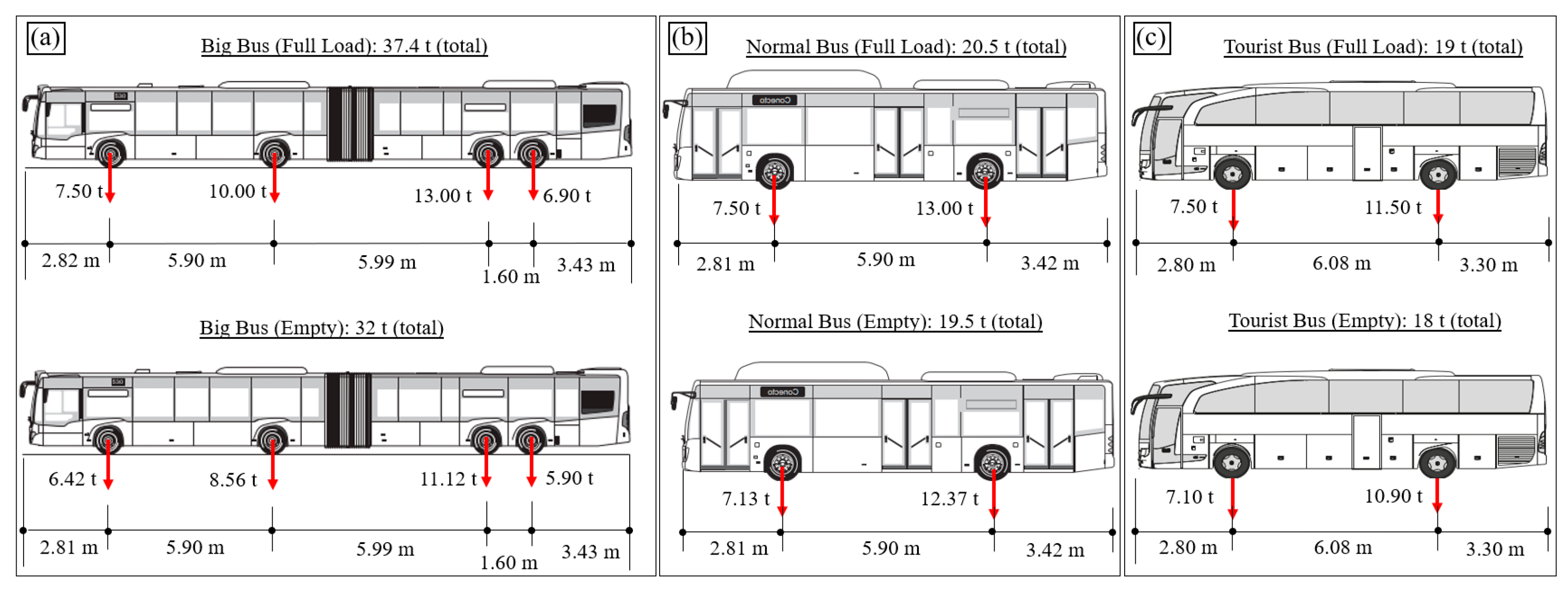
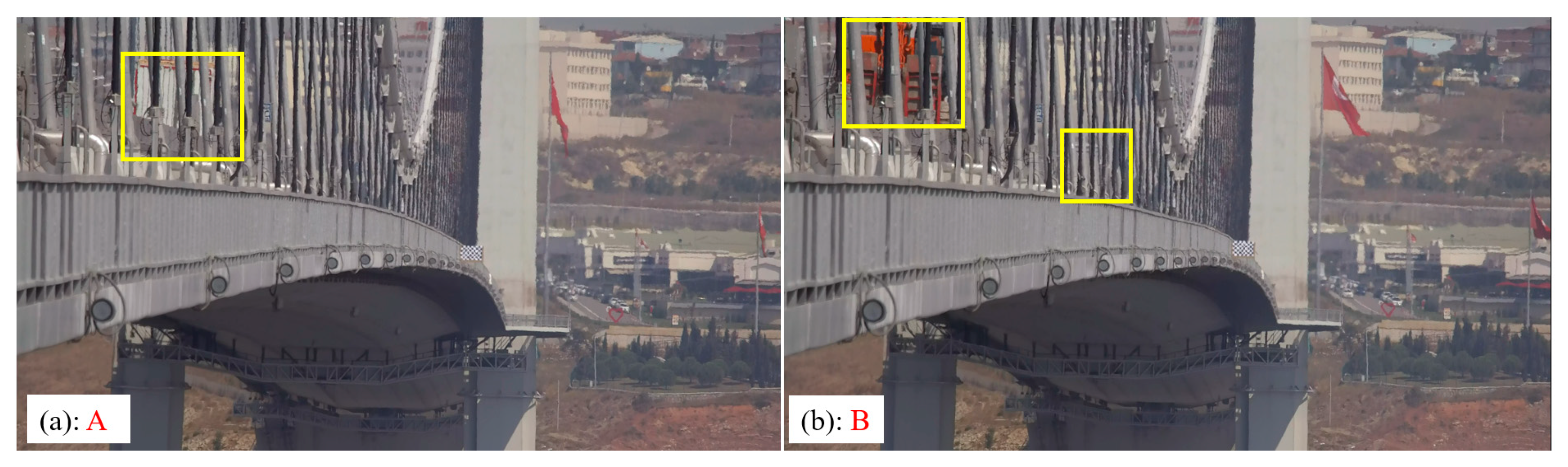
| Traffic Event | FE Case No. | FE Case Description | FE Evaluation (mm) | Computer Vision (mm) |
|---|---|---|---|---|
| A | 1 | 3 big buses (full) + 2 tourist buses (full) + no car | 241 | 428 |
| 2 | 3 big buses (empty) + 2 tourist buses (empty) + no car | 211 | ||
| 3 | 3 big buses (full) + 2 tourist buses (full) + cars | 408 | ||
| 4 | 3 big buses (empty) + 2 tourist buses (empty) + cars | 379 | ||
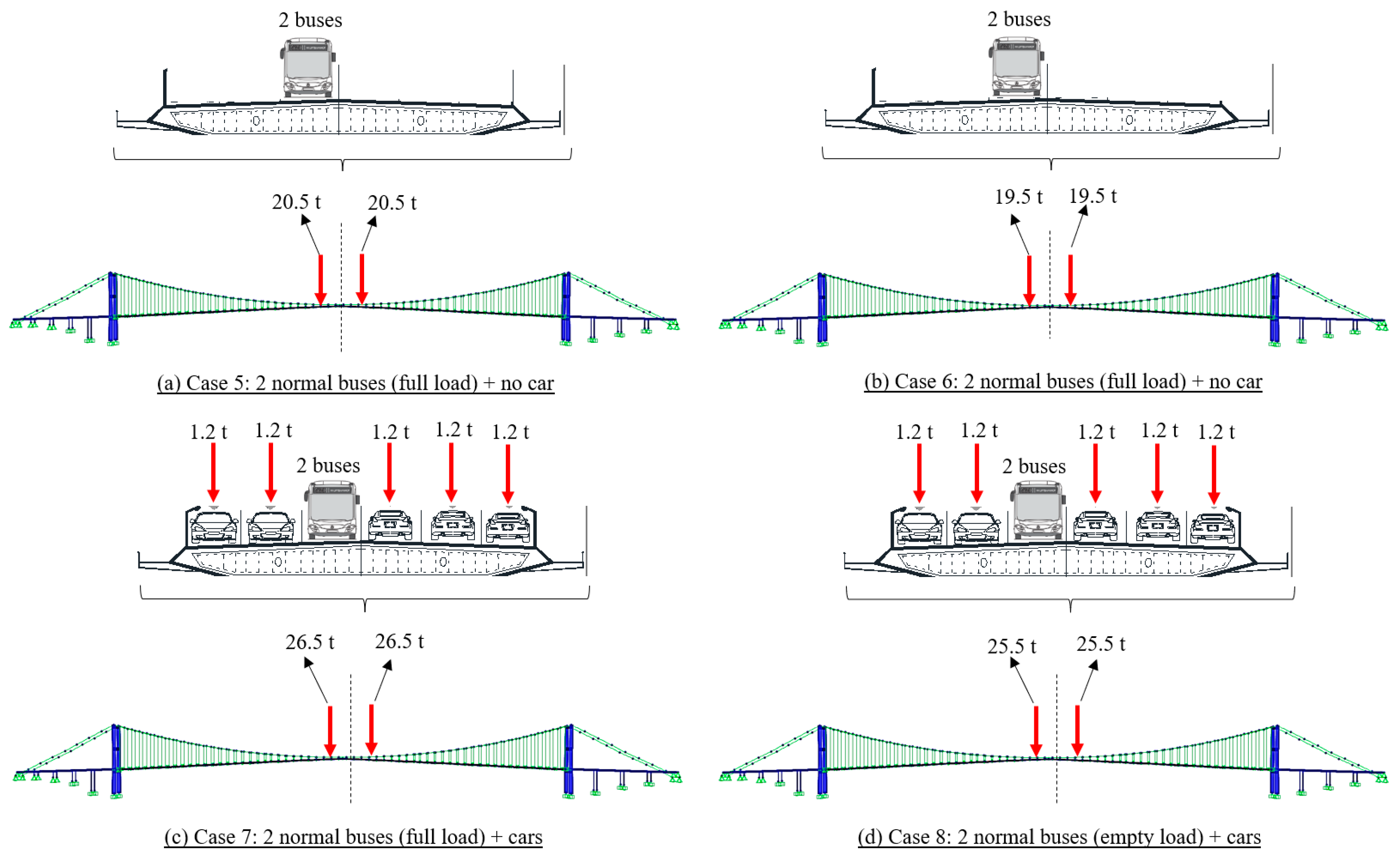
| B | 5 | 2 normal buses (full) + no car | 78 | 108 |
| 6 | 2 normal buses (empty) + no car | 75 | ||
| 7 | 2 normal buses (full) + cars | 102 | ||
| 8 | 2 normal buses (empty) + cars | 98 |
Disclaimer/Publisher’s Note: The statements, opinions and data contained in all publications are solely those of the individual author(s) and contributor(s) and not of MDPI and/or the editor(s). MDPI and/or the editor(s) disclaim responsibility for any injury to people or property resulting from any ideas, methods, instructions or products referred to in the content. |
© 2023 by the authors. Licensee MDPI, Basel, Switzerland. This article is an open access article distributed under the terms and conditions of the Creative Commons Attribution (CC BY) license (https://creativecommons.org/licenses/by/4.0/).
Share and Cite
Dong, C.; Bas, S.; Catbas, F.N. Applications of Computer Vision-Based Structural Monitoring on Long-Span Bridges in Turkey. Sensors 2023, 23, 8161. https://doi.org/10.3390/s23198161
Dong C, Bas S, Catbas FN. Applications of Computer Vision-Based Structural Monitoring on Long-Span Bridges in Turkey. Sensors. 2023; 23(19):8161. https://doi.org/10.3390/s23198161
Chicago/Turabian StyleDong, Chuanzhi, Selcuk Bas, and Fikret Necati Catbas. 2023. "Applications of Computer Vision-Based Structural Monitoring on Long-Span Bridges in Turkey" Sensors 23, no. 19: 8161. https://doi.org/10.3390/s23198161
APA StyleDong, C., Bas, S., & Catbas, F. N. (2023). Applications of Computer Vision-Based Structural Monitoring on Long-Span Bridges in Turkey. Sensors, 23(19), 8161. https://doi.org/10.3390/s23198161