Abstract
This paper investigates the power control and resource allocation problem in a simultaneously wireless information and power transfer (SWIPT)-based cognitive two-way relay network, in which two secondary users exchange information through a power splitting (PS) energy harvesting (EH) cognitive relay node underlay in a primary network. To enhance the secondary networks’s transmission ability without detriment to the primary network, we formulate an optimization to maximize the minimum transmission rates of the cognitive users by jointly optimizing power allocation at the sources, the time allocation of transmission frames and power splitting at the relay, under the constraint that the transmission power of the cognitive network is set not to exceed the primary user interference threshold to ensure primary work performance. To efficiently solve this problem, a sub-optimal algorithm named the joint power control and resource allocation (JPCRA) scheme is proposed, in which we decouple the non-convex problem into convex problems and use alternative steps in the optimization algorithm to get final solutions. Numerical results reveal that the proposed scheme enhances transmission fairness and outperforms three traditional schemes.
1. Introduction
The demand for spectrum resources is increasing rapidly as wireless communication continues to develop. However, the limited spectrum resources severely restrict the further growth of communication capacity. Cognitive radio is an effective technology to enhance spectrum efficiency through the reasonable reuse of the authorized spectrum. The technology mainly includes three modes: spectrum interweave, spectrum overlay and spectrum underlay [1,2]. Compared with interweave and overlay, underlay is simple to implement because no spectrum sensing is needed, and it has a better ability to realize spectrum sharing [3]. With underlay, in order to ensure a high priority of the primary user’s (PU) access of the spectrum, the transmit power of the cognitive users must be kept under the interference tolerance threshold of the PU. Therefore, power control becomes a key issue in optimizing the overall performance of the cognitive network [4].
In [5], Lee et al. investigate transmit power control for an underlay cognitive radio network by using a deep learning method that determines its own transmit power based solely on its local channel state information (CSI). In [6], Sarvendranath et al. develop an optimal and novel joint antenna selection and power adaptation rule that minimizes the average symbol error probability of a secondary user that is subject to two practically well-motivated constraints. Hu et al. [7] propose two optimal power control schemes from the long-term and short-term perspectives for a cognitive low orbit satellite constellation with terrestrial networks, which aims to maximize the delay-limited capacity and minimize the outage probability, respectively. In [8], Chuang et al. propose a dynamic multiobjective approach for power and spectrum allocation in a cognitive-based environment and propose a dynamic resource allocation algorithm comprising a hybrid initialization method and feasible point generation mechanisms to solve the dynamic multiobjective optimization problem. In [9], two efficient and low-complexity power control strategies are proposed for an ambient backscatter-based spectrum-sharing network, and with the backscatter prominent, there is no need to estimate all users’ CSI.
The relay technique can expand the transmission distance and improve the transmission reliability of the system. Integrating relay and cognitive techniques can further improve the transmission performance of the system [10,11]. In [12], the closed-form expression of outage probability for a cognitive multi-hop relay network is derived over Rayleigh fading channels, and an optimization problem to minimize the outage probability of the cognitive relay network is formulated and solved. In [13], a novel decentralized scheduling technique is developed for the cognitive multi-user multi-relay network, which operates on an incremental relaying mechanism and derives the outage probability of the secondary network for both the decode-and-forward (DF) and amplify-and-forward (AF) strategies. The transmission performance of a two-way AF cognitive relay network considering the influence of the primary network is studied in [14], and closed-forms of outage probability and bit error rate are derived. In [15], Yang et al. propose a dynamic power transmission scheme for non-orthogonal multiple access (NOMA) cognitive relay networks and derive the closed-form expressions of outage probability and average sum rate. Zhong and Zhang investigate relay selection in a two-way full-duplex AF relay network [16] and derive the system outage probability and bit error rate. In [17], Poornima et al. investigate the energy efficiency and the spectral efficiency performance of multi-hop full duplex cognitive relay networks.
Relaying often causes energy consumption issues, and forcing idle users to use their own energy to help the relay is difficult. Therefore, the energy issue in cognitive relay networks has become a topic of substantial research interest [18]. Introducing radio frequency (RF) wireless energy harvesting (EH) technology into cognitive relay networks could potentially solve both the energy and spectrum problems, which has attracted significant attention in the academic communities [19]. In [20], He et al. derive and compare the outage probabilities of the primary network and the EH cognitive network under direct transmission, single-user cooperation and multi-user cooperation scenarios. In [21], Shome et al. investigate the error probability of an energy harvesting co-operative cognitive radio network with several relay selection criteria. Wang et al. [22] study an energy harvesting-based secure transmission scheme for cognitive multi-relay networks and analyze the average secrecy rate, the secondary secrecy outage probability and the ergodic secrecy rate. More recently, some researchers have begun to study the SWIPT protocols and resource allocation for cognitive AF two-way relay networks [23,24]. The optimization model of [23] aims to maximize the total transmission throughput of the system, and the authors propose an algorithm by optimizing the transmit power of sensor nodes. In [24], the approximate closed-form expression of minimizing the outage probability and throughput is taken as the optimization objective, and the closed-form solution of the optimal power control parameters and power partition ratio are obtained. Shukla et al. [25] evaluate the performance of the proposed SWIPT-enabled NOMA system by considering both the perfect and imperfect successive interference cancellation for the legitimate users over Nakagami-m fading in terms of outage probability, system throughput and energy efficiency.
However, to the best of our knowledge, much of the previous references that emphasize performance optimization for an energy harvesting cognitive two-way relay network focus on the AF transmission protocol. On the other hand, the fairness issue and the interference effects of the main network on the secondary network are seldom studied. In our previous studies [26], we have investigated the power allocation under power control for a simultaneous wireless information and power transfer (SWIPT)-based cognitive two-way relay network with rate fairness consideration. However, the time allocation and power splitting issue have not been considered yet. In this paper, we consider the two-way DF cognitive relay network and investigate the jointly-optimum design based on the PS energy harvesting protocol, which aims to maximize the minimum cognitive user transmission rate with rate fairness and power control consideration. We achieve this by jointly optimizing the power allocation at source nodes, the time allocation of frames and the power splitting ratio at the relay. The main contributions are summarized as follows.
- (1)
- We develop a joint optimization scheme to maximize the minimum cognitive user transmission rate under rate fairness and power control consideration. The goal is to maximize the minimum cognitive user transmission performance through the joint optimization of time, power and power component ratio.
- (2)
- A stepped alternating optimization algorithm is proposed to solve the complex non-convex optimization problem. Through decoupling, the original problem is transformed into convex optimization problems and an alternating optimization problem. This avoids solving the complex non-convex optimization problem.
- (3)
- The results show that the proposed scheme improves the unfairness of inter-user transmission caused by channel asymmetry, and its superiority over the traditional scheme in terms of outage probability is depicted.
The rest of this paper is organized as follows: Section 2 presents the system model and problem formulation. Section 3 proposes the joint power control and resource allocation scheme. Section 4 studies and compares the performance of the proposed scheme under a simulation system setup. Finally, Section 5 concludes the paper.
2. System Model and Problem Formulation
Consider a half-duplex two-way cognitive relay network that consists of two source nodes and with a fixed power supply and a passive relay node with energy harvesting ability. All the terminals are equipped with a single omnidirectional antenna, and the antenna gain is normalized to 1. It is assumed that a direct link between the source nodes does not exist. We adopt the power splitting receiver architecture and DF protocol at relay. The system model is as shown in Figure 1.
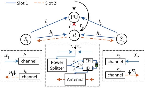
Figure 1.
System model for two-way cognitive relay network.
The information exchange of the whole transmission needs two time slots: a multiple access (MA) transmission phase and a broadcast (BC) phase. During the MA phase, source nodes and transmit their own information to relay R. Due to the broadcasting nature, PU receives the information from source nodes and as interference. To ensure the performance of the primary network, an interference threshold to restrict the total transmission power of source nodes and is set. Once the relay receives the signal, it partitions it into two parts: one part for energy harvesting, the other for information decoding. In the BC phase, the relay forwards the decoded signals to source nodes and with the harvested energy. Similarly, to ensure the performance of the primary network, the transmission power of the relay should be under the interference threshold.
2.1. Information and Energy Transfer
Let the total time of the whole transmission phase be normalized to be 1; if the MA phase time period is t, then the BC phase time period is . In the MA phase, the transmit power of each source node is . Due to the peak power constraint, should satisfied the following equation:
where is the peak power of source node .
Since the cognitive network utilizes underlay spectrum sharing, the received interference power for the primary user should be less than an interference threshold Q to satisfy the primary performance, i.e.,
where is the CSI from source to PU, and is the interference caused by spectrum sharing from source node to PU.
Let be the interference constraint ratio of two cognitive sources to the primary network. The restrictions of and can be reformulated as follows.
The signal received at the cognitive relay is
where is the interference introduced by the primary network, is the CSI between source node and the relay R, and is the white noise at the receiver.
The cognitive relay then splits the received signal into two parts: for energy harvesting and for information decoding. With linear energy harvesting, the harvested energy can be expressed as
where is energy conversion efficiency. Because for practical cases the noise power is far less than the signal power, we neglect white noise for simplicity of analysis. Thus, Equation (6) is written as
The signal used to decode information is written as
where is the noise generated by signal conversion from band-pass to baseband [27]. Since , in practice, for simplicity, we neglect in the following analysis.
According to Equation (8) and [10], the rate region of the MA phase is obtained as
where , is the signal to interference plus noise power ratio (SINR) from source to relay R, is the SINR of multiple access transmission, and
where , and .
In the broadcast phase, the cognitive relay performs information decoding utilizing the harvested energy. Assuming perfect CSI, the relay can utilize physical layer network coding to encode the received signal into . Because of underlay spectrum sharing, the transmit power of relay R is restricted not only by the harvested energy but also by the interference threshold of PU, which is written as
Equation (13) can be rewritten in a simpler form as
The signal received at source node is
where is the interference caused by the primary network, is white noise at source node .
Source node decodes and then uses self-cancellation to decode the intended information. For example, source node decodes : . According to Equation (16) and [10], the rate region of the BC phase is obtained as
where and are the SINRs from the relay to and , respectively, and are written as
2.2. Max-Min Optimization Problem Formulation
The goal is to assess the system’s potential transmission capability with fairness consideration for the cognitive SWIPT-based relay network. The primary network’s transmission should be guaranteed first. To this end, we propose joint power control and resource allocation optimization, aiming at maximizing the minimum transmission rate of the cognitive relay system. The optimization problem is formulated as
where , and are, respectively, the transmission power limits of the source nodes and relay; and are the transmission rate region limits of the MA phase and the BC phase, respectively; and , and are the range of the time allocation parameter, the range of the power splitting parameter and the range of the power control parameter, respectively.
Since multiple variables are coupled in conditions C2∼C4, OP1 is non-convex. Analysis reveals that when and are fixed, OP1 degenerates to a joint optimization problem determined by t and ; when t and are fixed, OP1 degenerates to an optimization problem determined by . Thus, the original problem can be decoupled into two parts deriving the optimal power control and power allocation parameters when t and are fixed and deriving the time allocation and power splitting parameters with joint resource allocation when the transmission power is fixed. Based on the analysis, we develop a sub-optimal algorithm to solve this complex problem.
3. Joint Power Control and Resource Allocation
A sub-optimal algorithm to solve OP1 is proposed, which is named joint power control and resource (JPCRA) allocation. It is based on solving two degenerated optimization works: power allocation with power control (PAPC) consideration and jointly optimum time allocation and power splitting ratio (JoTAPS) with a fixed transmit power. The final results can be obtained by using the alternative optimization algorithm based on PAPC and JoTAPS. This technique is described in detail next.
3.1. Power Allocation with Power Control Consideration
One degenerated optimization work is proposing a power allocation scheme that considers power control, i.e., deriving the optimal power control and power allocation parameters when t and are fixed. Equations (9) and (17) show that as or increases, the achievable upper bound of the objection function in the MA phase increases monotonically. As increases, in the BC phase increases monotonically. Thus, the system achieves optimal transmission performance with the maximum attainable values of , and expressed as
Equations (21)–(23) show that , and depend on . When the sources have no transmit power limits, , and can be rewritten as
By substituting Equations (24)–(26) into OP1, the optimization problem reduces to a one-dimensional optimization problem. Define . This one-dimensional optimization problem can be expressed as
where
and
Once the upper-bound of and as well as the intersection of and are determined, the optimal value of OP2 can be obtained by . Thus, the first step is to find , which maximizes and . Through some mathematical analysis, OP2 can be solved in the following two cases by comparing the two terms of expressed in Equation (32).
(1) Case 1: When
In this case, , the upper bound of is a constant that is not affected by ; the upper bound of is a continuous piecewise function of . The element in is a monotonically-increasing function of , and the element in is a monotonically-decreasing function of . is a monotonic function of whose monotony is affected by the value of . Denote as the intersection of and , as the intersection of and . The obtained that maximizes is
Since the upper bound of is not affected by , is a feasible solution for maximizing the upper bound of and even . Therefore, the optimal power control parameter of OP2 in Case 1 is .
(2) Case 2: When
In this case, . Substituting into OP2, we have
where
In this case, the upper bound of is a monotonically increasing function of , which is affected by the value of ; the upper bound of is a continuous piecewise function of , in which is a monotonically increasing function of while is a monotonically decreasing function, and is a monotonic function of affected by the value of . Denote as the intersection of and , as the intersection of and and as the intersection of and . Some analysis leads to the following observations:
- (a)
- WhenIn this case, and are constants. Thus, OP3 has one and only one optimal , .
- (b)
- WhenIn this case, and become monotonically increasing functions of . By analyzing the relationship of the intersection, can obtain that
- (c)
- WhenIn this case, and become monotonically decreasing functions. By analyzing the relationship of the intersection, one can obtain thatwhere , .
The above analysis leads to the optimal power control parameter, which satisfies OP2 under Case 2 as
Combining the optimal power control parameters of Case 1 and Case 2, we have the following optimal power control solution:
Next, we assume a fixed t and to derive the optimal power allocation ratio using the derived optimal power control parameters and the peak power limit of the source nodes. The derived theorem is described in Theorem 1.
Theorem 1.
For fixed parameters t and ρ, the optimal power allocation ratio that satisfies OP1 is obtained as
where is the optimal power control parameter that maximizes the minimum cognitive user transmission rate without considering the source peak power limits, , , , , and .
Proof.
When a limit on the source’s peak power is not enforced, the source transmit power can be written as , with optimum value . With a peak power constraint, and are separated into four cases based on the value of according to Equations (21)–(22):
- B1:
- when , ,
- B2:
- when , ,
- B3:
- when , ,
- B4:
- when , , .
The power allocation algorithm with fixed t and is given in Algorithm 1.
| Algorithm 1 Power allocation under power control with fixed t and . |
|
3.2. Optimal JoTAPS Scheme
This subsection derives the jointly optimum time allocation and power splitting ratio (JoTAPS) with a fixed transmit power. Firstly, we give an initial power control parameter . Then, the source nodes can determine the transmit power according to Equations (21) and (22), which are for and for . In this case, the previous optimization problem transforms into
By combining Equations (15) and (17), the rate region of the BC phase and the relay transmit power limit can be rewritten as
where
Define . The constraint of rate region and can be rewritten as
where
Some analysis reveals that with respect to (fix t) or with respect to t (fix ), OP4 is a convex optimization problem.
Theorem 2.
Given , OP4 is a convex optimization problem with respect to ρ (fix t) or with respect to t (fix ρ).
Proof.
To prove that OP4 is a convex optimization problem, we need to prove that the objective function and the constraint are both convex or affine functions. The objective function of OP4 is a constant, and when t and are fixed, is a linear function. Then, we derive the convex function properties of and .
When t is fixed, the first and second derivatives of in with respect to are
where , , are three cases of .
Since t is fixed, . Thus , , . From the properties of convex functions, we conclude that if and are convex (or concave) functions, then are convex (or concave) as well. Clearly is concave with respect to when t is fixed; thus, is concave with respect to .
When t is fixed, the first and second derivatives of in with respect to are
where , .
Since t is fixed, , . Thus, we can conclude that is concave with respect to , and so is with respect to .
Now, we analyze the case when is fixed. In this case, is a linear function. The second derivative of is
where .
Thus, OP4 is a concave function with respect to (when fixing t) or with respect to t (when fixing ). Theorem 2 is proved. □
Based on Theorem 2, we propose an alternating iterative optimization algorithm to determine optimal value of t and . The first step of the algorithm is to solve for the optimal with a given t. Let k be the iteration number. We can calculate the optimal value of the iteration by solving OP5-a, which is written as
Then, by substituting the optimal value of the kth iterations into OP5, the optimal value of the kth iterations can be calculated by solving OP5-b, which is written as
Since OP5-a and OP5-b are convex optimization problems, the value of and in each iteration can be solved by using CVX toolbox. With the solved and , an alternative algorithm named jointly-optimum time allocation and power splitting (JoTAPS) is designed as shown in Algorithm 2, where is the given allowable deviation.
| Algorithm 2 The jointly-optimum time and power splitting scheme with fixed power allocation algorithm |
|
3.3. Joint Power Control and Resource Allocation
Based on Algorithms 1 and 2, a stepped alternative optimization algorithm to solve OP1 is proposed. The idea of the algorithm is as follows:
Step 1: Give an initial power allocation ratio.
Step 2: Utilize Algorithm 2 to obtain the optimal power splitting ratio and time allocation ratio .
Step 3: Substitute the obtained and as the initial value of Algorithm 1 to obtain the power allocation ratio.
Finally, the optimized parameter value of OP1 is satisfied by solving the above three steps iteratively. The proposed algorithm is described below.
| Algorithm 3 Joint power control and resource allocation scheme |
|
4. Numerical Results and Discussions
In this section, we provide simulation results to evaluate the proposed joint power control and resource allocation (JPCRA) scheme. Based on the above derivation, we notice that the system parameters such as interference threshold, power and PU interference value have an effect on the max–min achievable rate . Thus, in the simulation part, we first simulate and analyze the effects of these parameters on in Figure 2, Figure 3 and Figure 4. To better demonstrate the superiority of the proposed JPCRA scheme, we compare it with the end-to-end achievable rates in Figure 5 and compare with three traditional optimization schemes in Figure 6, Figure 7 and Figure 8. The three traditional optimization schemes are the joint optimal power splitting and power allocation with fix time (FT-JoPSPA) scheme, joint optimal time and power allocation with fix power splitting (FPS-JoTPA) scheme and joint optimal time and power splitting with fix power allocation (FPA-JoTPS) scheme.
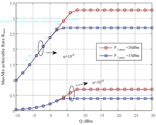
Figure 2.
The max–min achievable rate vs. the interference threshold of PU.
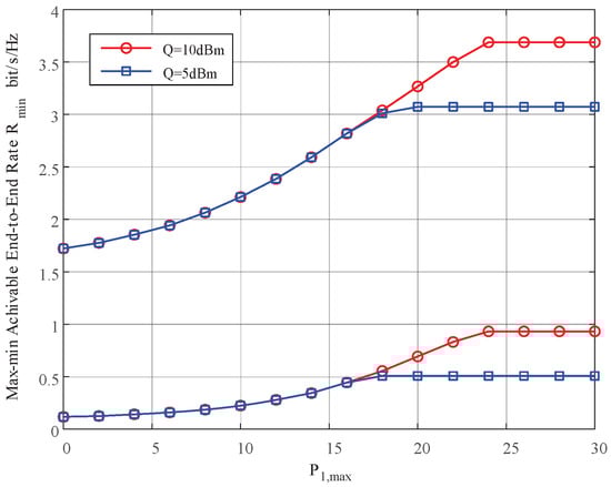
Figure 3.
The max–min achievable rate vs. the maximum transmit power constraint of .
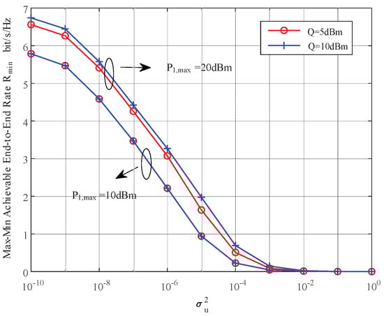
Figure 4.
The max–min achievable rate vs. the interference to the cognitive network caused by PU.
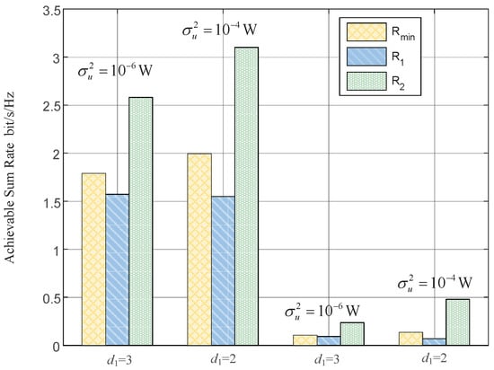
Figure 5.
The max–min achievable rate vs. the end-to-end achievable rates aiming at maximizing the achievable sum rate.
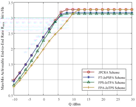
Figure 6.
The max–min rates of different optimization schemes vs. the interference threshold of PU.
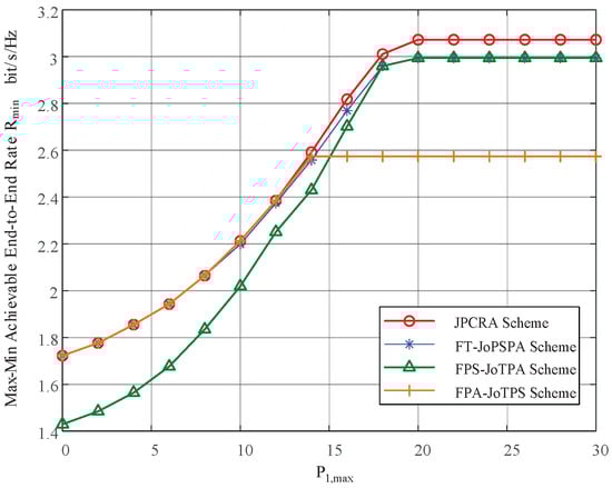
Figure 7.
The max–min rates of different optimization schemes vs. the transmit power constraint of .
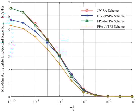
Figure 8.
The max–min rates of different optimization schemes vs. the transmit power constraint of .
4.1. Simulation Setup and Parameters
The effectiveness of our proposed scheme is evaluated through experimental simulations in which the full-band urban indoor communication environment is taken into account. Let be the distances between the source and relay R, let be the distances between the source to primary user PU and let be the distances between relay node to PU, respectively. We consider , and as the channel gains between source and relay R, between source and the PU and between the relay node and the PU, respectively, where is the pass loss exponent. The channel gains between two nodes are reciprocal. To simplify the analysis, we consider a case where the sources and the relay are on a straight line, with m and m. The interference effects from the PU to each secondary users are assumed to be the same, i.e., . The noise power is given as W. Since full-band communication is considered, the frequency band is normalized as . The parameters used in the simulation part are listed in Table 1.

Table 1.
The parameters used in the simulation part.
4.2. The Effects of Parameters on
The efficiency of the parameter settings in the proposed technique is investigated according to the following figures.
Figure 2 depicts the influence of the interference tolerance threshold on the max–min cognitive user achievable rate. The simulation parameters are (3, 7) m, (20, 15) dBm, dBm, W. It is observed that when Q increases to a certain value, initially increases and eventually saturates because the transmission rate of the cognitive user is a monotonically increasing function of transmit power which is affected by Q and the peak power constraint. When Q is sufficiently small, the transmit power is mainly limited by Q. When Q increases to a certain value (larger than the peak power), the transmit power is determined mainly by the peak power. Thus, increasing Q cannot continuously improve the achievable sum-rate.
Figure 3 depicts the the max–min achievable rate versus the peak power of source when (3, 7) m, (5, 10) dBm, 15 dBm and . The result shows that increases and tends to saturate to a stable value as increases to a certain value. This is because is proportional to the user’s transmission power, and the cognitive user transmission power is affected by Q and at the same time. When is small, the user’s transmit power is limited by . Thus, increases as . As increases to a certain value (larger than Q), however, the user’s transmit power is limited by Q. Thus, continuing to increase will not change .
Figure 4 depicts the max–min achievable rate obtained by the proposed JPCRA scheme versus the interference power caused by the primary user to cognitive user when (3, 7) m, (5, 10) dBm, (20, 15) dBm, 15 dBm. It can be seen that decreases and approaches 0 as increases, and the descend degree of JPCRA is more gradual. Thus, consideration of the interference from the primary network is necessary to design the cognitive energy harvesting system.
4.3. Performance Analysis with Comparative Schemes
The superiority of the proposed scheme with benchmark schemes is investigated according to the following figures.
Figure 5 compares the max–min achievable rate () obtained by the proposed JPCRA scheme with the end-to-end rate (we use to denote the transmission rate of source () obtained by the maximization of achievable sum-rate (MASR) scheme [28]. In the simulation, parameters are set as {2, 3} m, {2, 3} m, (15, 15) dBm and W. This figure clearly shows that increases as decreases while remains the same, and also increases, because the system with MASR scheme will enhance the transmission ability of the high channel quality to maximize the achievable sum-rate. Thus, the MASR scheme cannot enhance the transmission ability of the poor channel, which may mean that the transmission links with a poor channel quality do not meet their transmission needs. The proposed scheme considers the transmission fairness, effectively alleviating the effects caused by channel asymmetry. Therefore, when the system values the enhancement of the worst performance of a user most in this system, it is better to choose the proposed JPCRA scheme, whereas when the system values the enhancement of the system achievable sum rate most, it is better to choose the MASR scheme.
Figure 6 depicts the max–min achievable rate of the proposed JPCRA scheme versus the interference threshold of the primary network, which is compared with three traditional transmission schemes. The parameters are set as (3, 7) m, = 20 dBm, 15 dBm, W. It is observed that as the interference threshold increases, the of each scheme increases and saturates at a stable value. This is because the transmit power of the cognitive user is mainly constrained by power control when the interference threshold is small; as the interference threshold increases to a certain value, the transmit power of the cognitive user is mainly constrained by the peak power limits. In this figure, the peak power is a fixed parameter; thus, the performance saturates as the interference threshold increases to a certain value. The proposed JPCRA scheme outperforms the other three schemes in the whole range of Q. When the interference threshold is a high SNR value, it is possible to use the FPA-JoTPS scheme to replace JPCRA, and when the interference threshold is a low SNR value, it is possible to use the FT-JoPSPA scheme to replace JPCRA.
Figure 7 shows the max–min achievable rate versus peak transmit power limit . The proposed JPCRA scheme is compared with three traditional transmission schemes. The parameters are set as (3, 7) m, 5 dBm, = 15 dBm and W. The proposed JPCRA scheme clearly outperforms the three other schemes. It is also observed that as increases, the of each schemes increases and saturates to a stable value. This is because the transmit power is curved by the PU threshold, which curves the transmission rates. In this figure, it can be seen that when the peak transmit power limit is sufficient, the proposed JPCRA scheme is definitely a good choice, whereas when is in the low-SNR range, it is possible to use the three other traditional schemes to replace JPCRA.
Figure 8 illustrates the max–min achievable rate versus the interference power caused by the primary user to cognitive user. The parameters are set as (3, 7) m, 5 dBm, = 20 dBm and = 15 dBm. As increases, decreases and approaches 0. The proposed JPCRA scheme outperforms the other three schemes, and the smaller is, the greater the performance gap, while a smaller results in a greater impact of resource allocation. Considering the influence of on system performance, the primary user with less influence on the secondary network interference should be selected for spectrum sharing when selecting spectrum sharing objects.
4.4. Results Discussion
In this study, we investigate the performance of the proposed JPCRA scheme from two aspects. Firstly, the impact of parameter settings on the max–min achievable rate is investigated. We verify that the performance growth of is curved by the interference threshold of PU and the maximum transmit power constraint that echoes the cognitive two-way relay network should guarantee the performance of the primary network primarily. Then, the performance of the JPCRA scheme is compared with the MASR scheme, showing that the JPCRA scheme is preferable to enhance the poor channel quality. Last but not least, the superiority of the JPCRA scheme is verified compared with three traditional optimization schemes (FT-JoPSPA, FPS-JoTPA, FPA-JoTPS), which shows that the proposed JPCRA scheme achieves high performance in the whole range of adjustable SNR (changing Q, or , or ).
5. Conclusions
We have studied the power control and resource allocation problem in the energy harvesting cognitive two-way relay network using the PS protocol and DF relay forwarding protocol. By considering transmission fairness, a joint resource allocation problem under power control is established, which aims at maximizing the minimum transmission rates of the cognitive users. To solve the optimization problem, a stepped alternative optimization algorithm, named the JPCRA scheme, is proposed to obtain the optimal parameter values. Simulation results have shown that the proposed scheme can improve the transmission performance of the cognitive users with poor channel quality and have verified its superiority compared with three other traditional schemes.
Further, we intend to expand the proposed scheme in an indoor relay environment or unmanned aerial vehicle cognitive relay circumstance. Another interesting further research direction could be exploring deep learning for cognitive relay selection.
Author Contributions
The main contributions of C.P. and G.W. were to create the main ideas and execute performance evaluations by theoretical analysis and simulation, while H.L. worked as the cooperator to discuss, create and advise on the main ideas and performance evaluations. All authors have read and agreed to the published version of the manuscript.
Funding
This work is supported in part by the Science and Technology Research Project of Chongqing Education Commission under Grant KJQN201901103 and KJQN202003106 and KJQN202103111, in part by the innovation research group of universities in Chongqing under Grant CXQT21035, in part by the innovation research group of Chongqing University of Technology under Grant 2023TDZ014, in part by the Research Start-up Fund of Chongqing University of Technology under Grant 2019ZD127 and in part by the Incubation Program of National Natural Science Foundation of China under Grant 2021PYZ10.
Institutional Review Board Statement
Not applicable.
Informed Consent Statement
Informed consent was obtained from all subjects involved in the study.
Data Availability Statement
The data is unavailable due to privacy or ethical restrictions.
Acknowledgments
The authors would like to thank Yi Huang, a lecture in Chongqing College of Electronic Engineering, who took part in the discussion of mathematical methodology and helped to carry out the simulation debugging and analysis.
Conflicts of Interest
The authors declare no conflict of interest.
Abbreviations
The following abbreviations are used in this manuscript:
| SWIPT | Simultaneous wireless information and power transfer |
| JPCRA | Joint power control and resource allocation |
| PU | Primary user |
| NOMA | Non-orthogonal multiple access |
| AF | Amplify-and-forward |
| DF | Decoded-and-forward |
| RF | Radio frequency |
| PS | Power splitting |
| EH | Energy harvesting |
| MA | Multiple access |
| BC | Broadcast |
| CSI | Channel state information |
| SINR | Signal to interference plus noise power ratio |
| JoTAPS | Optimum time allocation and power splitting ratio |
| PAPC | Power allocation with power control |
| JoTAPS | Jointly optimum time allocation and power splitting ratio |
| FT-JoPSPA | Joint optimal power splitting and power allocation with fix time |
| FPS-JoTPA | Joint optimal time and power allocation with fix power splitting |
| FPA-JoTPS | Joint optimal time and power splitting with fix power allocation |
References
- Tsiropoulos, G.I.; Dobre, O.A.; Ahmed, M.H.; Baddour, K.E. Radio Resource Allocation Techniques for Efficient Spectrum Access in Cognitive Radio Networks. IEEE Commun. Surv. Tutor. 2016, 18, 824–847. [Google Scholar] [CrossRef]
- Biswas, S.; Bishnu, A.; Khan, F.A.; Ratnarajah, T. In-Band Full-Duplex Dynamic Spectrum Sharing in Beyond 5G Networks. IEEE Commun. Mag. 2021, 59, 54–60. [Google Scholar] [CrossRef]
- Wu, W.; Wang, Z.; Yuan, L.; Zhou, F.; Lang, F.; Wang, B.; Wu, Q. IRS-Enhanced Energy Detection for Spectrum Sensing in Cognitive Radio Networks. IEEE Wirel. Commun. Lett. 2021, 10, 2254–2258. [Google Scholar] [CrossRef]
- Gupta, M.; Prakriya, S. Performance of CSI-Based Power Control and NOMA/OMA Switching for Uplink Underlay Networks With Imperfect SIC. IEEE Trans. Cog. Commun. Net. 2022, 8, 1753–1769. [Google Scholar] [CrossRef]
- Lee, W.; Lee, K. Deep Learning-Aided Distributed Transmit Power Control for Underlay Cognitive Radio Network. IEEE Trans.Veh. Tech. 2021, 70, 3990–3994. [Google Scholar] [CrossRef]
- Sarvendranath, R.; Mehta, N.B. Exploiting Power Adaptation With Transmit Antenna Selection for Interference-Outage Constrained Underlay Spectrum Sharing. IEEE Trans. Commun. 2020, 68, 480–492. [Google Scholar] [CrossRef]
- Hu, J.; Li, G.; Bian, D.; Gou, L.; Wang, C. Optimal Power Control for Cognitive LEO Constellation with Terrestrial Networks. IEEE Commun. Lett. 2020, 24, 622–625. [Google Scholar] [CrossRef]
- Chuang, C.L.; Chiu, W.Y.; Chuang, Y.C. Dynamic Multiobjective Approach for Power and Spectrum Allocation in Cognitive Radio Networks. IEEE Syst. J. 2021, 15, 5417–5428. [Google Scholar] [CrossRef]
- Hu, Z.; Yang, S.; Zhang, Z. Ambient Backscatter-Based Power Control Strategies for Spectrum Sharing Networks. IEEE Trans. Cog. Commun. Net. 2022, 8, 1848–1861. [Google Scholar] [CrossRef]
- Kim, S.J.; Devroye, N.; Mitran, P.; Tarokh, V. Achievable Rate Regions and Performance Comparison of Half Duplex Bi-Directional Relaying Protocols. IEEE Trans. Inf. Theory 2011, 57, 6405–6418. [Google Scholar] [CrossRef]
- Uyoata, U.; Mwangama, J.; Adeogun, R. Relaying in the Internet of Things (IoT): A Survey. IEEE Access 2021, 9, 132675–132704. [Google Scholar] [CrossRef]
- Xie, F.; Zou, Y.; Zhu, J.; Chen, K. Power Allocation for Minimizing Outage Probability of Cognitive Multi-Hop Relay Networks. In Proceedings of the International Conference on Wireless Communications and Signal Processing (WCSP), Changsha, China, 20–21 October 2021; pp. 1–6. [Google Scholar]
- Kandelusy, O.M.; Kirsch, N.J. Cognitive Multi-User Multi-Relay Network: A Decentralized Scheduling Technique. IEEE Trans. Cog. Commun. Net. 2011, 7, 609–623. [Google Scholar] [CrossRef]
- Vahidian, S.; Soleimani-Nasab, E.; Aissa, S.; Ahmadian-Attari, M. Bidirectional AF Relaying With Underlay Spectrum Sharing in Cognitive Radio Networks. IEEE Trans. Veh. Tech. 2017, 66, 2367–2381. [Google Scholar] [CrossRef]
- Yang, Z.; Hussein, J.A.; Xu, P.; Chen, G.; Wu, Y.; Ding, Z. Performance Study of Cognitive Relay NOMA Networks with Dynamic Power Transmission. IEEE Trans. Veh. Tech. 2021, 70, 2882–2887. [Google Scholar] [CrossRef]
- Zhong, B.; Zhang, Z. Opportunistic Two-Way Full-Duplex Relay Selection in Underlay Cognitive Networks. IEEE Syst. J. 2018, 12, 725–734. [Google Scholar] [CrossRef]
- Poornima, S.; Babu, A.V. Power Adaptation for Enhancing Spectral Efficiency and Energy Efficiency in Multi-Hop Full Duplex Cognitive Wireless Relay Networks. IEEE Trans. Mob. Comput. 2022, 21, 2143–2157. [Google Scholar]
- Feng, D.; Jiang, C.; Lim, G.; Cimini, L.J.; Feng, G.; Li, G.Y. A survey of energy-efficient wireless communications. IEEE Commun. Surv. Tutor. 2013, 15, 167–178. [Google Scholar] [CrossRef]
- Lu, X.; Wang, P.; Niyato, D.; Kim, D.I.; Han, Z. Wireless Networks With RF Energy Harvesting: A Contemporary Survey. IEEE Commun. Surv. Tutor. 2015, 17, 757–789. [Google Scholar] [CrossRef]
- He, J.; Guo, S.; Pan, G.; Yang, Y.; Liu, D. Relay Cooperation and Outage Analysis in Cognitive Radio Networks With Energy Harvesting. IEEE Syst. J. 2018, 12, 2129–2140. [Google Scholar] [CrossRef]
- Shome, A.; Dutta, A.K.; Chakrabarti, S. BER Performance Analysis of Energy Harvesting Underlay Cooperative Cognitive Radio Network With Randomly Located Primary Users and Secondary Relays. IEEE Trans. Veh. Tech. 2021, 70, 4740–4752. [Google Scholar] [CrossRef]
- Hossain, M.A.; Noor, R.M.; Yau, K.-L.A.; Ahmedy, I.; Anjum, S.S. A Survey on Simultaneous Wireless Information and Power Transfer with Cooperative Relay and Future Challenges. IEEE Access 2019, 7, 19166–19198. [Google Scholar] [CrossRef]
- Yang, C.; Lu, W.; Huang, G.; Qian, L.; Li, B.; Gong, Y. Power Optimization in Two-way AF Relaying SWIPT based Cognitive Sensor Networks. In Proceedings of the IEEE Vehicular Technology Conference (VTC2020-Fall), Victoria, BC, Canada, 16–18 November 2020; pp. 1–5. [Google Scholar]
- Singh, S.; Modem, S.; Prakriya, S. Optimization of Cognitive Two-Way Networks With Energy Harvesting Relays. IEEE Commun. Lett. 2017, 21, 1381–1384. [Google Scholar] [CrossRef]
- Shukla, A.K.; Sharanya, J.; Yadav, K.; Upadhyay, P.K. Exploiting SWIPT-Enabled IoT-Based Cognitive Nonorthogonal Multiple Access With Coordinated Direct and Relay Transmission. IEEE Sens. J. 2022, 22, 18988–18999. [Google Scholar] [CrossRef]
- Wang, G.; Peng, C.; Huang, Y. The Power Allocation for SWIPT-based Cognitive Two-Way Relay Networks with Rate Fairness Consideration. In Proceedings of the IEEE International Conference on Trust, Security and Privacy in Computing and Communications (TrustCom), Wuhan, China, 9–11 December 2022; pp. 60–65. [Google Scholar]
- Nasir, A.A.; Zhou, X.; Durrani, S.; Kennedy, R.A. Relaying Protocols for Wireless Energy Harvesting and Information Processing. IEEE Trans. Wirel. Commun. 2013, 12, 3622–3636. [Google Scholar] [CrossRef]
- Peng, C.; Li, F.; Liu, H. Optimal Power Splitting in Two-Way Decode-and-Forward Relay Networks. IEEE Commun. Lett. 2017, 21, 2009–2012. [Google Scholar] [CrossRef]
Disclaimer/Publisher’s Note: The statements, opinions and data contained in all publications are solely those of the individual author(s) and contributor(s) and not of MDPI and/or the editor(s). MDPI and/or the editor(s) disclaim responsibility for any injury to people or property resulting from any ideas, methods, instructions or products referred to in the content. |
© 2023 by the authors. Licensee MDPI, Basel, Switzerland. This article is an open access article distributed under the terms and conditions of the Creative Commons Attribution (CC BY) license (https://creativecommons.org/licenses/by/4.0/).