
Qualitative Classification of Proximal Femoral Bone Using Geometric Features and Texture Analysis in Collected MRI Images for Bone Density Evaluation


Abstract
:1. Introduction
- The compilation of a comprehensive MRI database available for the diagnosis of osteoporosis;
- The provision of a smart algorithm based on machine learning techniques to evaluate bone density;
- Achievement of the highest detection speed for bone density assessment;
- A comparison of the proposed method with other deep learning methods.
2. Methods
2.1. Data Collection
- T1/TR = 415.00 ms/TE = 19.00 ms/Flip-Angle = 150 (44 referred, 33 healthy, 11 unhealthy)
- T1/TR = 536.00 ms/TE = 11.00 ms/Flip-Angle = 180 (43 referred, 31 healthy, 12 unhealthy)
- T1/TR = 4070.00 ms/TE = 33.00 ms/Flip-Angle = 180 (42 referred, 29 healthy, 13 unhealthy)
- T1/TR = 420.00 ms/TE = 22.00 ms/Flip-Angle = 180 (45 referred, 36 healthy, 9 unhealthy)
- T2/TR = 3600.00 ms/TE = 80.00 ms/Flip-Angle = 150 (45 referred, 19 healthy, 26 unhealthy)
- T2/TR = 7840.00 ms/TE = 109.00 ms/Flip-Angle = 150 (41 referred, 28 healthy, 13 unhealthy)
- T1/TR = 389.00 ms/TE = 13.42 ms/Flip-Angle = 110 (24 referred, 9 healthy, 15 unhealthy)
2.2. Programming Environment and Settings
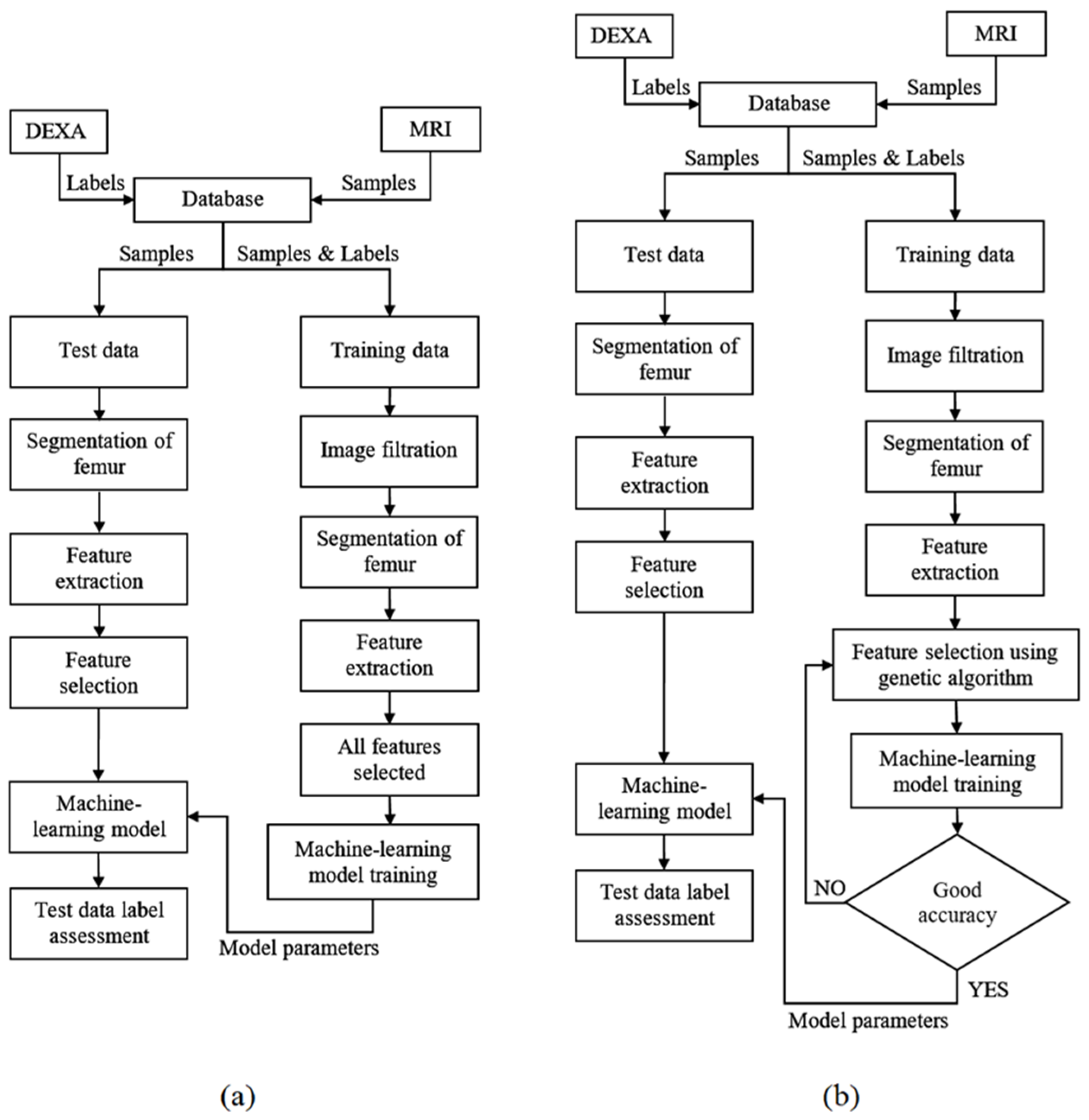
2.3. Overall Procedure
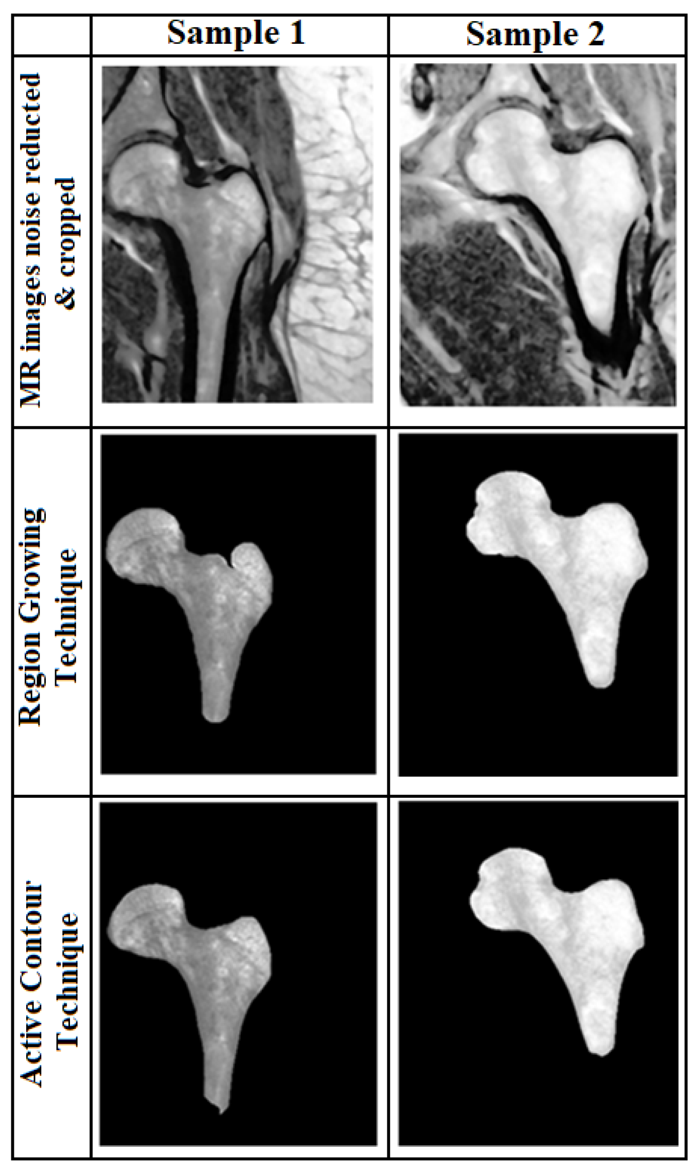
2.4. Segmentation
2.5. Classification Algorithms
2.5.1. Classification Using Decision Tree
2.5.2. Classification Using Logistic Regression
2.5.3. Classification Based on the SVM Algorithm
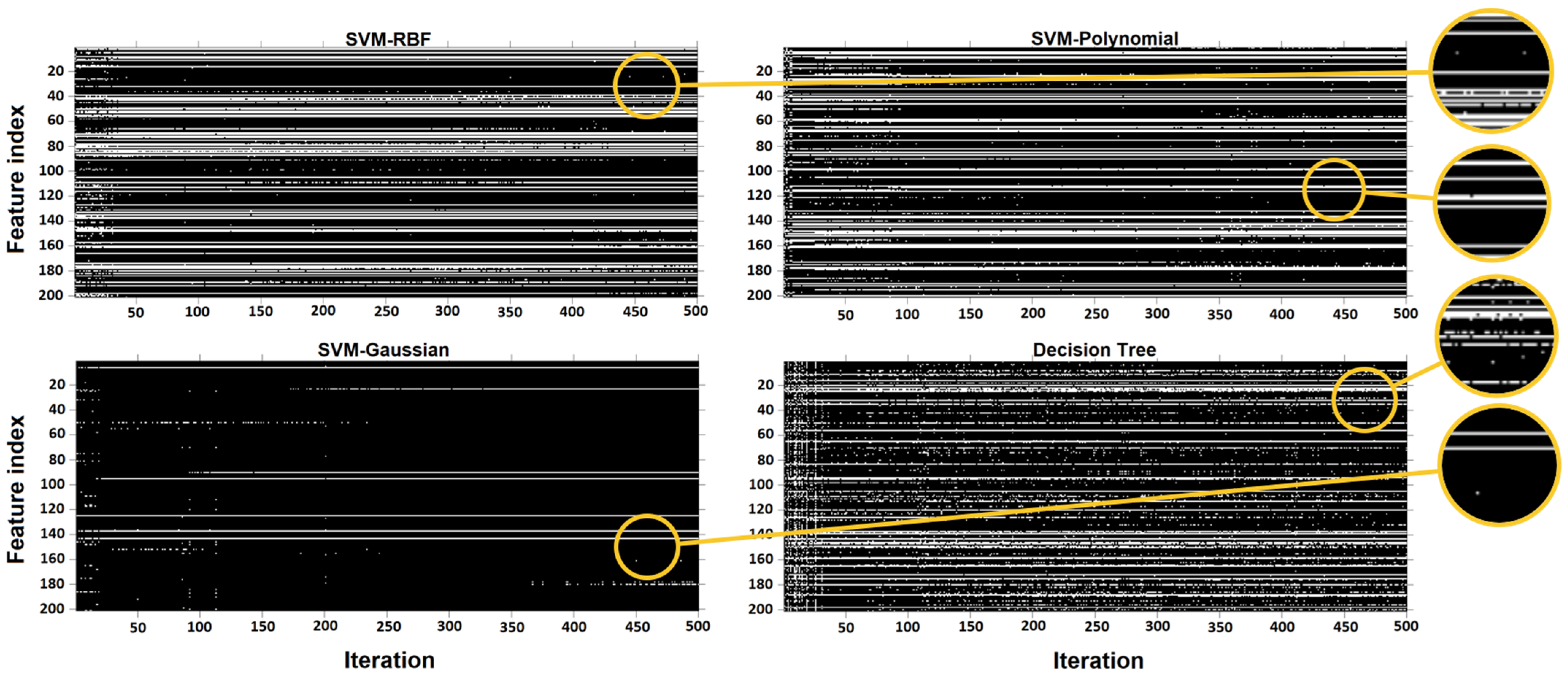
2.6. Feature Selection Using the Genetic Algorithm
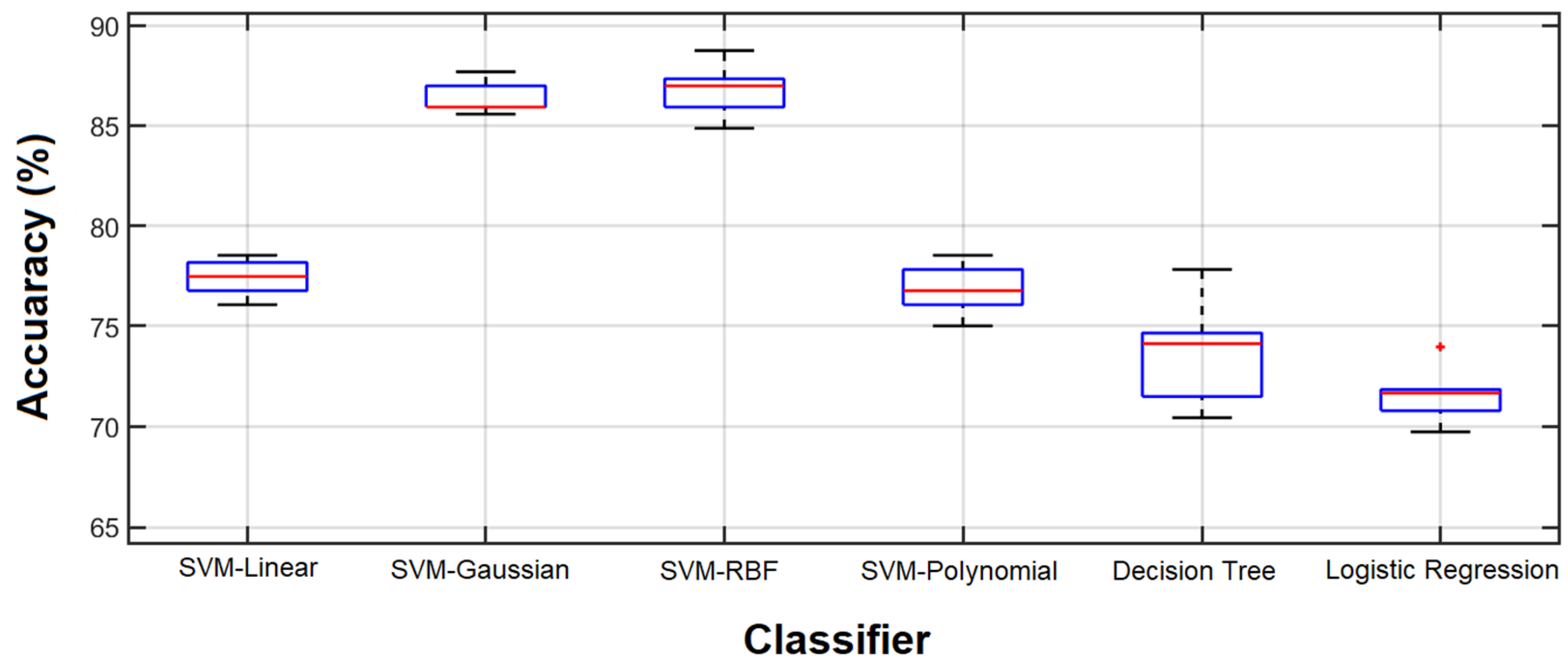
3. Results
4. Discussion
5. Conclusions
Author Contributions
Funding
Institutional Review Board Statement
Informed Consent Statement
Data Availability Statement
Acknowledgments
Conflicts of Interest
References
- Lei, C.; Song, J.-H.; Li, S.; Zhu, Y.-N.; Liu, M.-Y.; Wan, M.-C.; Mu, Z.; Tay, F.R.; Niu, L.-N. Advances in materials-based therapeutic strategies against osteoporosis. Biomaterials 2023, 296, 122066. [Google Scholar] [CrossRef] [PubMed]
- Yang, L.; Chen, C.; Zhang, Z.; Wei, X. Diagnosis of bone mineral density based on backscattering resonance phenomenon using coregistered functional laser photoacoustic and ultrasonic probes. Sensors 2021, 21, 8243. [Google Scholar] [CrossRef]
- Holubiac, I.Ș.; Leuciuc, F.V.; Crăciun, D.M.; Dobrescu, T. Effect of strength training protocol on bone mineral density for postmenopausal women with osteopenia/osteoporosis assessed by dual-energy x-ray absorptiometry (DEXA). Sensors 2022, 22, 1904. [Google Scholar] [CrossRef] [PubMed]
- Shahini, N.; Bahrami, Z.; Sheykhivand, S.; Marandi, S.; Danishvar, M.; Danishvar, S.; Roosta, Y. Automatically identified EEG signals of movement intention based on CNN network (End-To-End). Electronics 2022, 11, 3297. [Google Scholar] [CrossRef]
- Yu, W.; Xie, Z.; Li, J.; Lin, J.; Su, Z.; Che, Y.; Ye, F.; Zhang, Z.; Xu, P.; Zeng, Y. Super enhancers targeting ZBTB16 in osteogenesis protect against osteoporosis. Bone Res. 2023, 11, 30. [Google Scholar] [CrossRef]
- Wang, H.; Luo, Y.; Wang, H.; Li, F.; Yu, F.; Ye, L. Mechanistic advances in osteoporosis and anti-osteoporosis therapies. MedComm 2023, 4, e244. [Google Scholar] [CrossRef] [PubMed]
- Marcucci, G.; Domazetovic, V.; Nediani, C.; Ruzzolini, J.; Favre, C.; Brandi, M.L. Oxidative stress and natural antioxidants in osteoporosis: Novel preventive and therapeutic approaches. Antioxidants 2023, 12, 373. [Google Scholar] [CrossRef] [PubMed]
- Sabahi, K.; Sheykhivand, S.; Mousavi, Z.; Rajabioun, M. Recognition COVID-19 cases using deep type-2 fuzzy neural networks based on chest X-ray image. Comput. Intell. Electr. Eng. 2023, 14, 75–92. [Google Scholar]
- Al-Saleh, Y.; Sulimani, R.; Sabico, S.; Alshahrani, F.M.; Fouda, M.A.; Almohaya, M.; Alaidarous, S.B.; Alkhawashki, H.M.; Alshaker, M.; Alrayes, H. Diagnosis and management of osteoporosis in Saudi Arabia: 2023 key updates from the Saudi Osteoporosis Society. Arch. Osteoporos. 2023, 18, 75. [Google Scholar] [CrossRef] [PubMed]
- Tai, T.-W.; Huang, C.-F.; Huang, H.-K.; Yang, R.-S.; Chen, J.-F.; Cheng, T.-T.; Chen, F.-P.; Chen, C.-H.; Chang, Y.-F.; Hung, W.-C. Clinical practice guidelines for the prevention and treatment of osteoporosis in Taiwan: 2022 update. J. Formos. Med. Assoc. 2023, in press. [CrossRef]
- De Sire, A.; Lippi, L.; Venetis, K.; Morganti, S.; Sajjadi, E.; Curci, C.; Ammendolia, A.; Criscitiello, C.; Fusco, N.; Invernizzi, M. Efficacy of antiresorptive drugs on bone mineral density in post-menopausal women with early breast cancer receiving adjuvant aromatase inhibitors: A systematic review of randomized controlled trials. Front. Oncol. 2022, 11, 829875. [Google Scholar] [CrossRef]
- Ciancia, S.; Högler, W.; Sakkers, R.J.; Appelman-Dijkstra, N.M.; Boot, A.M.; Sas, T.C.; Renes, J.S. Osteoporosis in children and adolescents: How to treat and monitor? Eur. J. Pediatr. 2023, 182, 501–511. [Google Scholar] [CrossRef] [PubMed]
- Khare, M.R.; Havaldar, R.H. Non-invasive methodological techniques to determine health of a bone. In Techno-Societal 2020: Proceedings of the 3rd International Conference on Advanced Technologies for Societal Applications; Springer: Cham, Switzerland, 2021; Volume 1, pp. 343–350. [Google Scholar]
- Guerri, S.; Mercatelli, D.; Gómez, M.P.A.; Napoli, A.; Battista, G.; Guglielmi, G.; Bazzocchi, A. Quantitative imaging techniques for the assessment of osteoporosis and sarcopenia. Quant. Imaging Med. Surg. 2018, 8, 60. [Google Scholar] [CrossRef] [PubMed]
- Kanis, J.A.; McCloskey, E.V.; Harvey, N.C.; Cooper, C.; Rizzoli, R.; Dawson-Hughes, B.; Maggi, S.; Reginster, J.-Y. The need to distinguish intervention thresholds and diagnostic thresholds in the management of osteoporosis. Osteoporos. Int. 2023, 34, 1–9. [Google Scholar] [CrossRef] [PubMed]
- Lungaro, L.; Manza, F.; Costanzini, A.; Barbalinardo, M.; Gentili, D.; Caputo, F.; Guarino, M.; Zoli, G.; Volta, U.; De Giorgio, R. Osteoporosis and celiac disease: Updates and hidden pitfalls. Nutrients 2023, 15, 1089. [Google Scholar] [CrossRef]
- Han, M.; Chiba, K.; Banerjee, S.; Carballido-Gamio, J.; Krug, R. Variable flip angle three-dimensional fast spin-echo sequence combined with outer volume suppression for imaging trabecular bone structure of the proximal femur. J. Magn. Reson. Imaging 2015, 41, 1300–1310. [Google Scholar] [CrossRef]
- Dittrich, A.T.; Janssen, E.J.; Geelen, J.; Bouman, K.; Ward, L.M.; Draaisma, J.M. Diagnosis, Follow-Up and Therapy for Secondary Osteoporosis in Vulnerable Children: A Narrative Review. Appl. Sci. 2023, 13, 4491. [Google Scholar] [CrossRef]
- Sollmann, N.; Löffler, M.T.; Kronthaler, S.; Böhm, C.; Dieckmeyer, M.; Ruschke, S.; Kirschke, J.S.; Carballido-Gamio, J.; Karampinos, D.C.; Krug, R. MRI-based quantitative osteoporosis imaging at the spine and femur. J. Magn. Reson. Imaging 2021, 54, 12–35. [Google Scholar] [CrossRef]
- Deniz, C.M.; Xiang, S.; Hallyburton, R.S.; Welbeck, A.; Babb, J.S.; Honig, S.; Cho, K.; Chang, G. Segmentation of the proximal femur from MR images using deep convolutional neural networks. Sci. Rep. 2018, 8, 16485. [Google Scholar] [CrossRef]
- Sheykhivand, S.; Yousefi Rezaii, T.; Mousavi, Z.; Meshini, S. Automatic stage scoring of single-channel sleep EEG using CEEMD of genetic algorithm and neural network. Computational Intelligence in Electrical Engineering 2018, 9, 15–28. [Google Scholar]
- Dhanaji Kale, K.; Ainapure, B.; Nagulapati, S.; Sankpal, L.; Sambhajirao Satpute, B. Chronological-hybrid optimization enabled deep learning for boundary segmentation and osteoporosis classification using femur bone. Imaging Sci. J. 2023. [Google Scholar] [CrossRef]
- Franco-Gonçalo, P.; Pereira, A.I.; Loureiro, C.; Alves-Pimenta, S.; Filipe, V.; Gonçalves, L.; Colaço, B.; Leite, P.; McEvoy, F.; Ginja, M. Femoral Neck Thickness Index as an Indicator of Proximal Femur Bone Modeling. Vet. Sci. 2023, 10, 371. [Google Scholar] [CrossRef] [PubMed]
- Dolz, J.; Desrosiers, C.; Ayed, I.B. 3D fully convolutional networks for subcortical segmentation in MRI: A large-scale study. NeuroImage 2018, 170, 456–470. [Google Scholar] [CrossRef] [PubMed]
- Ong, W.; Zhu, L.; Tan, Y.L.; Teo, E.C.; Tan, J.H.; Kumar, N.; Vellayappan, B.A.; Ooi, B.C.; Quek, S.T.; Makmur, A. Application of Machine Learning for Differentiating Bone Malignancy on Imaging: A Systematic Review. Cancers 2023, 15, 1837. [Google Scholar] [CrossRef]
- Chay, Z.E.; Lee, C.H.; Lee, K.C.; Oon, J.S.; Ling, M.H. Russel and Rao coefficient is a suitable substitute for Dice coefficient in studying restriction mapped genetic distances of Escherichia coli. arXiv 2023, arXiv:2302.12714. [Google Scholar]
- Qingyun, F.; Zhaokui, W. Fusion Detection via Distance-Decay Intersection over Union and Weighted Dempster–Shafer Evidence Theory. J. Aerosp. Inf. Syst. 2023, 20, 114–125. [Google Scholar] [CrossRef]
- Xu, Y.; Li, S.; Wang, Z.; Zhang, H.; Li, Z.; Xiao, B.; Guo, W.; Liu, L.; Bai, P. Design of multi-DC overdriving waveform of electrowetting displays for gray scale consistency. Micromachines 2023, 14, 684. [Google Scholar] [CrossRef]
- Lv, Z.; Li, J.; Li, X.; Wang, H.; Wang, P.; Li, L.; Shu, L.; Li, X. Two adaptive enhancement algorithms for high gray-scale RAW infrared images based on multi-scale fusion and chromatographic remapping. Infrared Phys. Technol. 2023, 133, 104774. [Google Scholar] [CrossRef]
- Tayefi, M.; Tajfard, M.; Saffar, S.; Hanachi, P.; Amirabadizadeh, A.R.; Esmaeily, H.; Taghipour, A.; Ferns, G.A.; Moohebati, M.; Ghayour-Mobarhan, M. hs-CRP is strongly associated with coronary heart disease (CHD): A data mining approach using decision tree algorithm. Comput. Methods Programs Biomed. 2017, 141, 105–109. [Google Scholar] [CrossRef]
- Yeo, B.; Grant, D. Predicting service industry performance using decision tree analysis. Int. J. Inf. Manag. 2018, 38, 288–300. [Google Scholar] [CrossRef]
- Makond, B.; Pornsawad, P.; Thawnashom, K. Decision Tree Modeling for Osteoporosis Screening in Postmenopausal Thai Women. Informatics 2022, 9, 83. [Google Scholar] [CrossRef]
- Louk, M.H.L.; Tama, B.A. Dual-IDS: A bagging-based gradient boosting decision tree model for network anomaly intrusion detection system. Expert Syst. Appl. 2023, 213, 119030. [Google Scholar] [CrossRef]
- Ambrish, G.; Ganesh, B.; Ganesh, A.; Srinivas, C.; Mensinkal, K. Logistic regression technique for prediction of cardiovascular disease. Glob. Transit. Proc. 2022, 3, 127–130. [Google Scholar]
- Hu, Y.; Fan, Y.; Song, Y.; Li, M. A general robust low–rank multinomial logistic regression for corrupted matrix data classification. Appl. Intell. 2023, 53, 18564–18580. [Google Scholar] [CrossRef]
- Gulati, K.; Kumar, S.S.; Boddu, R.S.K.; Sarvakar, K.; Sharma, D.K.; Nomani, M. Comparative analysis of machine learning-based classification models using sentiment classification of tweets related to COVID-19 pandemic. Mater. Today Proc. 2022, 51, 38–41. [Google Scholar] [CrossRef]
- Pitchai, R.; Supraja, P.; Sulthana, A.R.; Veeramakali, T.; Babu, C.M. MRI image analysis for cerebrum tumor detection and feature extraction using 2D U-ConvNet and SVM classification. Pers. Ubiquitous Comput. 2023, 27, 931–940. [Google Scholar] [CrossRef]
- Meng, X.; Wei, Q.; Meng, L.; Liu, J.; Wu, Y.; Liu, W. Feature fusion and detection in Alzheimer’s disease using a novel genetic multi-kernel SVM based on MRI imaging and gene data. Genes 2022, 13, 837. [Google Scholar] [CrossRef]
- Yoon, J.K.; Choi, J.-Y.; Rhee, H.; Park, Y.N. MRI features of histologic subtypes of hepatocellular carcinoma: Correlation with histologic, genetic, and molecular biologic classification. Eur. Radiol. 2022, 32, 5119–5133. [Google Scholar] [CrossRef]
- Liang, T.-O.; Koh, Y.H.; Qiu, T.; Li, E.; Yu, W.; Huang, S.Y. High-performance permanent magnet array design by a fast genetic algorithm (GA)-based optimization for low-field portable MRI. J. Magn. Reson. 2022, 345, 107309. [Google Scholar] [CrossRef]
- Do, D.T.; Yang, M.-R.; Lam, L.H.T.; Le, N.Q.K.; Wu, Y.-W. Improving MGMT methylation status prediction of glioblastoma through optimizing radiomics features using genetic algorithm-based machine learning approach. Sci. Rep. 2022, 12, 13412. [Google Scholar] [CrossRef]
- Bharati, S.; Podder, P.; Mondal, M.; Prasath, V. CO-ResNet: Optimized ResNet model for COVID-19 diagnosis from X-ray images. Int. J. Hybrid Intell. Syst. 2021, 17, 71–85. [Google Scholar] [CrossRef]
- Khaleghi, N.; Rezaii, T.Y.; Beheshti, S.; Meshgini, S.; Sheykhivand, S.; Danishvar, S. Visual saliency and image reconstruction from EEG signals via an effective geometric deep network-based generative adversarial network. Electronics 2022, 11, 3637. [Google Scholar] [CrossRef]
- Hajipour Khire Masjidi, B.; Bahmani, S.; Sharifi, F.; Peivandi, M.; Khosravani, M.; Hussein Mohammed, A. CT-ML: Diagnosis of breast cancer based on ultrasound images and time-dependent feature extraction methods using contourlet transformation and machine learning. Comput. Intell. Neurosci. 2022, 2022, 1493847. [Google Scholar] [CrossRef] [PubMed]
- Madanan, M.; Sayed, B.T. Designing a deep learning hybrid using CNN and Inception V3 transfer learning to detect the aggression level of deep obsessive compulsive disorder in children. Int. J. Biol. Biomed. Eng 2022, 16, 207–220. [Google Scholar] [CrossRef]
- Ferizi, U.; Besser, H.; Hysi, P.; Jacobs, J.; Rajapakse, C.S.; Chen, C.; Saha, P.K.; Honig, S.; Chang, G. Artificial intelligence applied to osteoporosis: A performance comparison of machine learning algorithms in predicting fragility fractures from MRI data. J. Magn. Reson. Imaging 2019, 49, 1029–1038. [Google Scholar] [CrossRef]


| Features | Description | No. of Features |
|---|---|---|
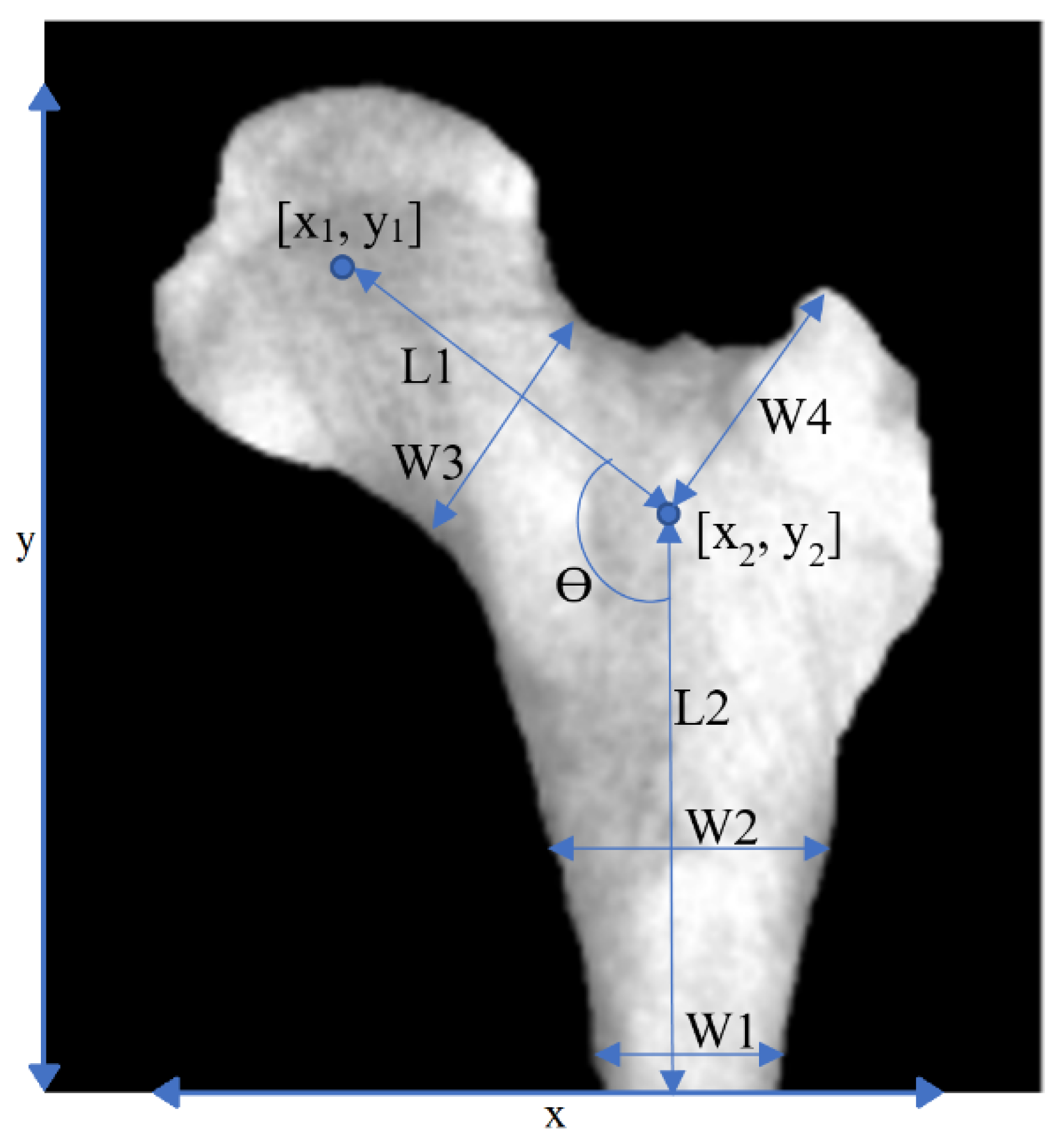
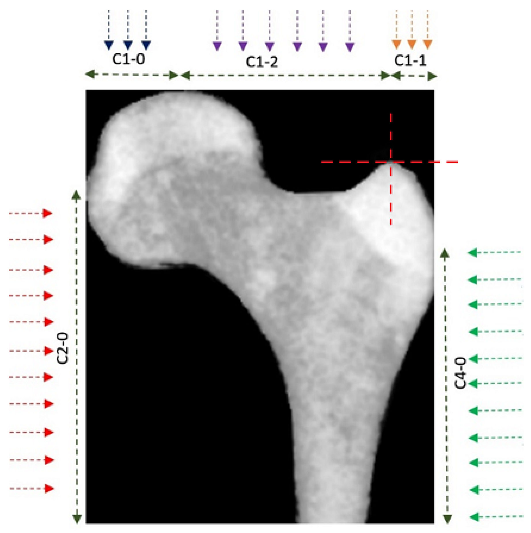
| Geometrical features | As in Figure 2, i.e.,: x1, y1, L1, L2, Ɵ, W0, W1, W2, W3,W4, x, y | 12 |
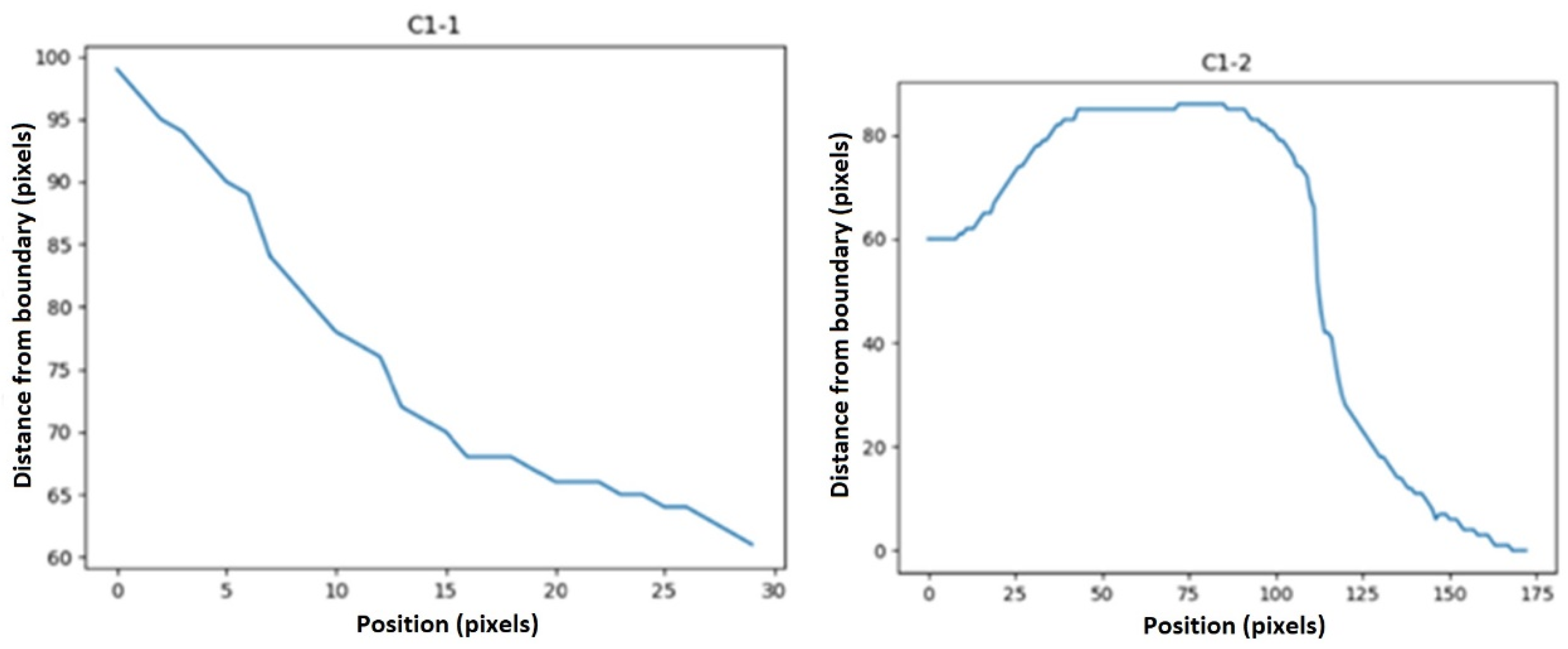
| C1-1 | min, max, average ramp, kurtosis (ramp_removed_sig), skew (ramp_removed_sig), first to last point ramp, moment1 (ramped_remov_sig), moment 2 (ramp_removed_sig), variance, max. of second derivative | 10 |
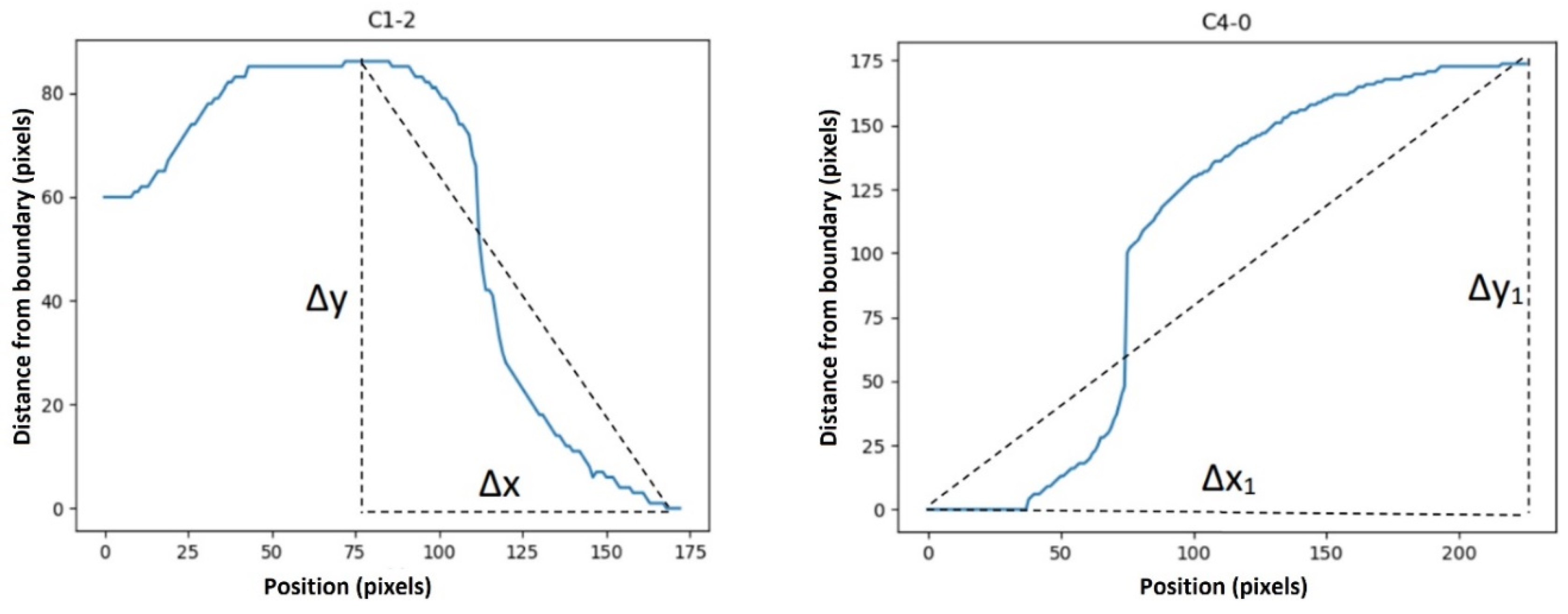
| C1-2 | min, max, mean, variance, kurtosis, skew, moment1, moment2 | 8 |
| C1-0 | min, max, average ramp, kurtosis (ramp_removed_sig), skew (ramp_removed_sig), first to last point ramp, moment1 (ramped_remov_sig), moment 2 (ramp_removed_sig), variance, max of second derivative | 10 |
| C2-0 | min, max, average ramp, kurtosis (ramp_removed_sig), skew (ramp_removed_sig), first to last point ramp, moment 1 (ramped_remov_sig), moment2 (ramp_removed_sig), variance, max of second derivative | 10 |
| C4-0 | min, max, average ramp, kurtosis (ramp_removed_sig), skew (ramp_removed_sig), first to last point ramp, moment1 (ramped_remov_sig), moment2 (ramp_removed_sig), variance, max of second derivative | 10 |
| Features based on texture | mean, variance, skew | 3 |
| Fractal dimensions | fractal dimensions | 1 |
| Features based on texture | gray-level co-occurrence matrix (GLCM) | 4 |
| Features | Classifier | TH | FH | TU | FU | Acc. (%) | F1 Score (%) | No. of Selected Features |
|---|---|---|---|---|---|---|---|---|
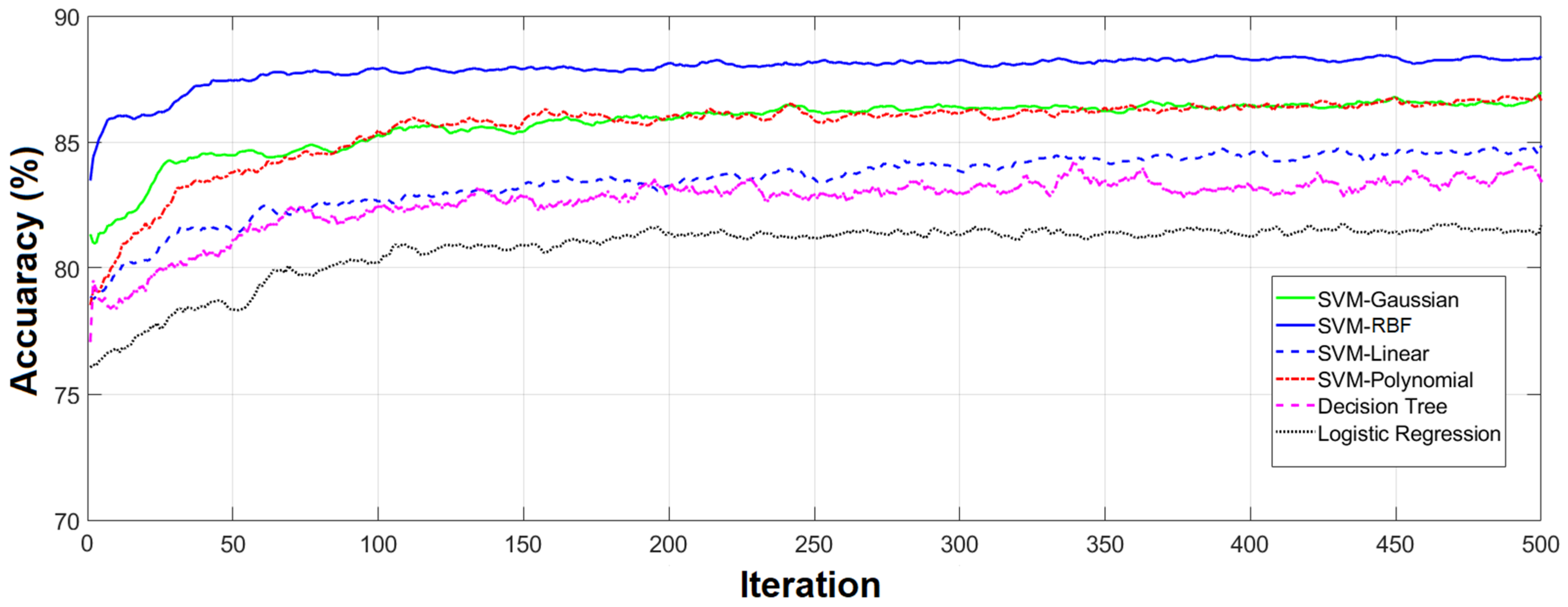
| Using selected features by the Genetic algorithm | SVM-Linear | 167 | 24 | 75 | 18 | 85.21 | 83.48 | 60 |
| SVM-RBF | 172 | 18 | 81 | 13 | 89.08 | 87.84 | 56 | |
| SVM-Gaussian | 173 | 24 | 75 | 12 | 87.32 | 85.61 | 7 | |
| SVM-Polynomial | 161 | 11 | 88 | 24 | 87.68 | 86.80 | 54 | |
| Decision Tree | 168 | 24 | 75 | 17 | 85.56 | 83.83 | 62 | |
| Logistic Regression | 158 | 24 | 75 | 27 | 82.04 | 80.37 | 80 |
| Methods | ACC. (%) | F1 Score (%) | Time per Iteration |
|---|---|---|---|
| ResNet17 | 89.05 | 87.14 | 4.2 s |
| VGG19 | 88.90 | 89.1 | 7.1 s |
| GoogleNet | 79.47 | 80.36 | 9 s |
| Inception v3 | 85.04 | 86.74 | 8.5 s |
| Proposed Model | 89.08 | 87.84 | 1 s |
Disclaimer/Publisher’s Note: The statements, opinions and data contained in all publications are solely those of the individual author(s) and contributor(s) and not of MDPI and/or the editor(s). MDPI and/or the editor(s) disclaim responsibility for any injury to people or property resulting from any ideas, methods, instructions or products referred to in the content. |
© 2023 by the authors. Licensee MDPI, Basel, Switzerland. This article is an open access article distributed under the terms and conditions of the Creative Commons Attribution (CC BY) license (https://creativecommons.org/licenses/by/4.0/).
Share and Cite
Najafi, M.; Yousefi Rezaii, T.; Danishvar, S.; Razavi, S.N. Qualitative Classification of Proximal Femoral Bone Using Geometric Features and Texture Analysis in Collected MRI Images for Bone Density Evaluation. Sensors 2023, 23, 7612. https://doi.org/10.3390/s23177612
Najafi M, Yousefi Rezaii T, Danishvar S, Razavi SN. Qualitative Classification of Proximal Femoral Bone Using Geometric Features and Texture Analysis in Collected MRI Images for Bone Density Evaluation. Sensors. 2023; 23(17):7612. https://doi.org/10.3390/s23177612
Chicago/Turabian StyleNajafi, Mojtaba, Tohid Yousefi Rezaii, Sebelan Danishvar, and Seyed Naser Razavi. 2023. "Qualitative Classification of Proximal Femoral Bone Using Geometric Features and Texture Analysis in Collected MRI Images for Bone Density Evaluation" Sensors 23, no. 17: 7612. https://doi.org/10.3390/s23177612
APA StyleNajafi, M., Yousefi Rezaii, T., Danishvar, S., & Razavi, S. N. (2023). Qualitative Classification of Proximal Femoral Bone Using Geometric Features and Texture Analysis in Collected MRI Images for Bone Density Evaluation. Sensors, 23(17), 7612. https://doi.org/10.3390/s23177612