
GRP-YOLOv5: An Improved Bearing Defect Detection Algorithm Based on YOLOv5


Abstract
:1. Introduction
- In the preprocessing stage, a gamma transformation preprocessing technique is introduced to perform a nonlinear transformation of the image’s grayscale values, thus enhancing the image’s contrast and brightness. This process eliminates the similarity between bearing defects and non-defective regions, reducing the occurrence of false positives and false negatives.
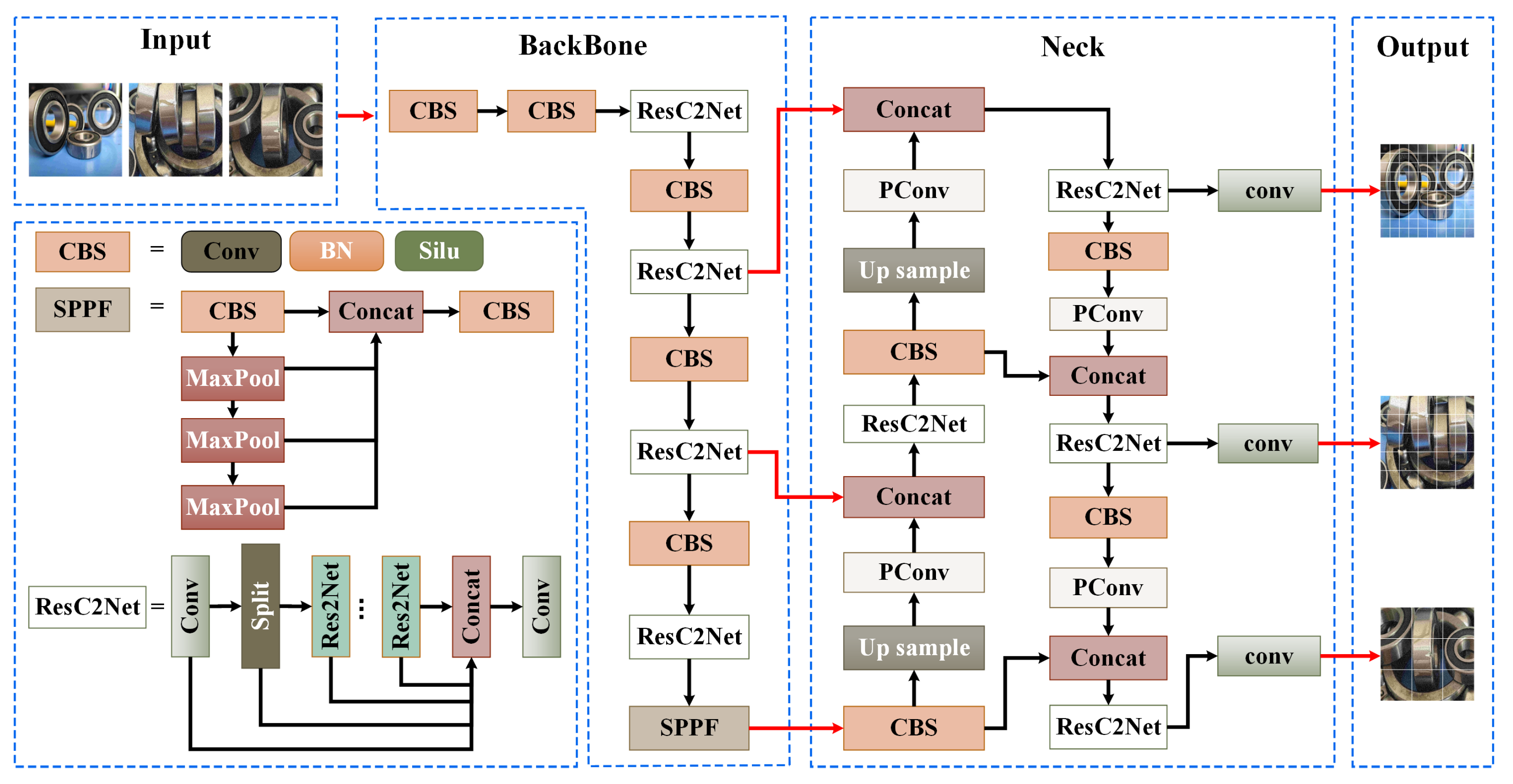
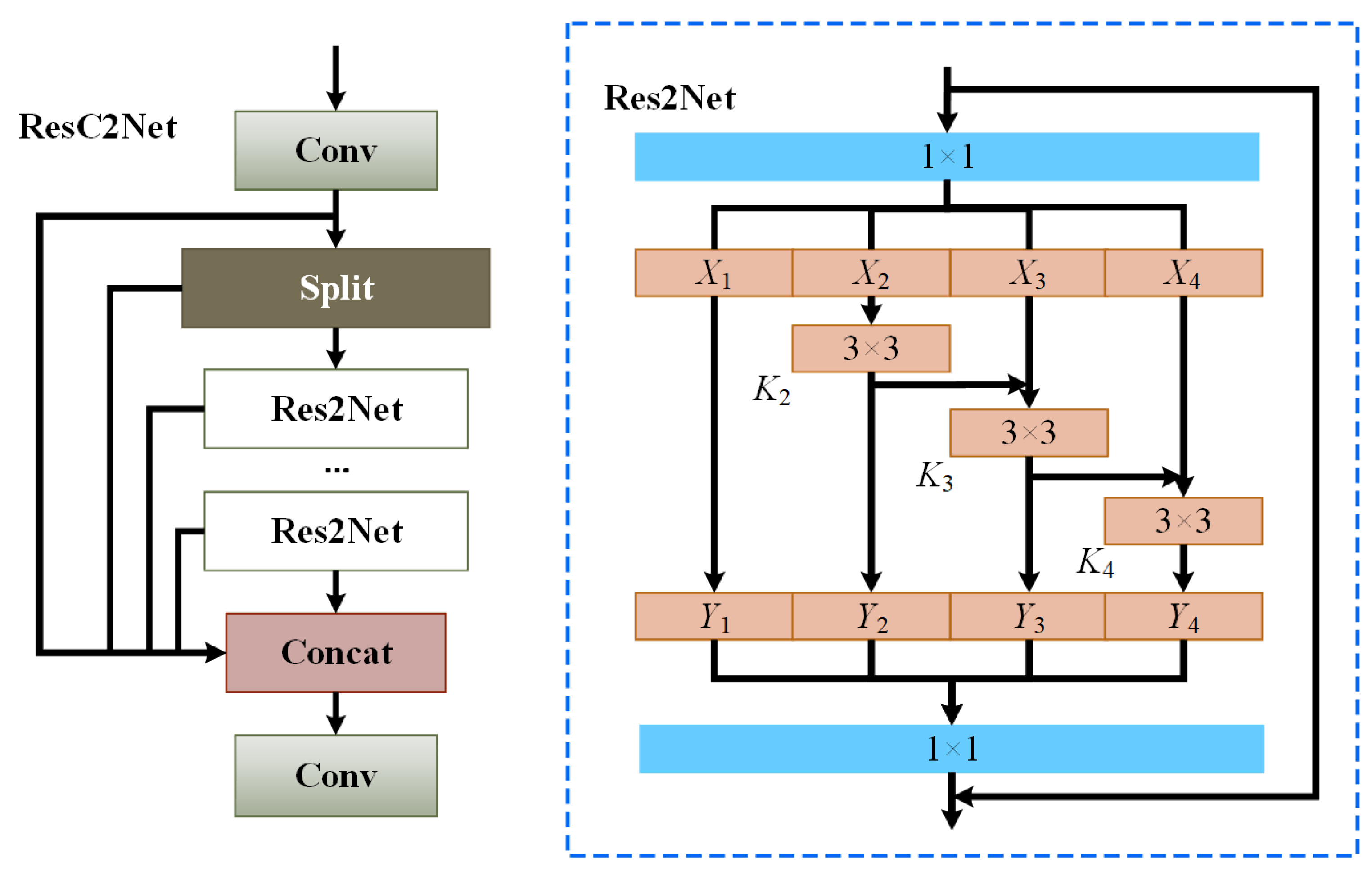
- In the backbone network, a novel ResC2Net residual-like network structure is proposed to enhance the network’s feature representation and attention enhancement capabilities, further improving the detection performance for small bearing defects.
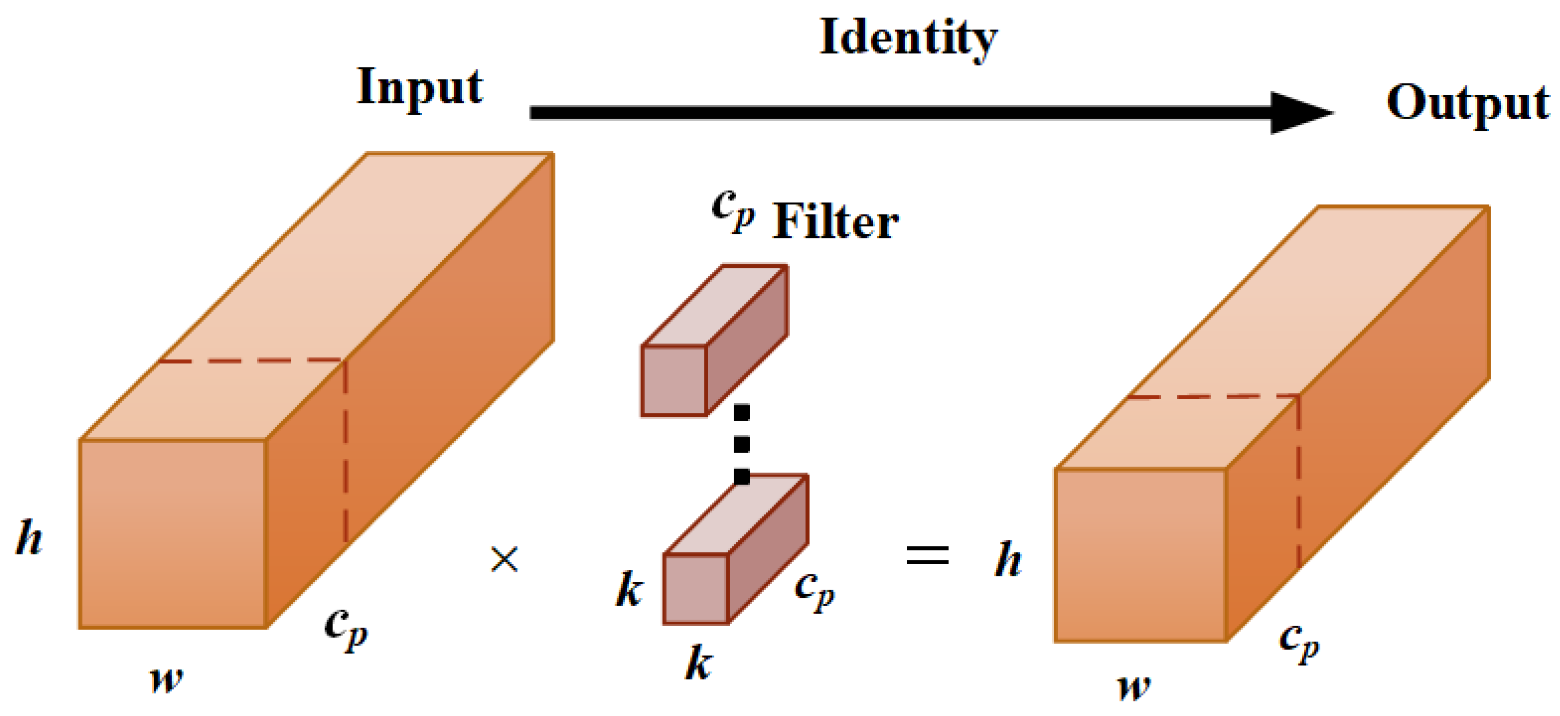
- In the model’s neck, a PConv local convolution operation is added to improve the accuracy of defect edge detection without increasing the computational complexity.
2. Research Status at Home and Abroad
2.1. Traditional Detection Methods
2.2. Deep Learning-Based Detection Methods
3. Algorithm Description
3.1. Data Preprocessing
3.2. Backbone
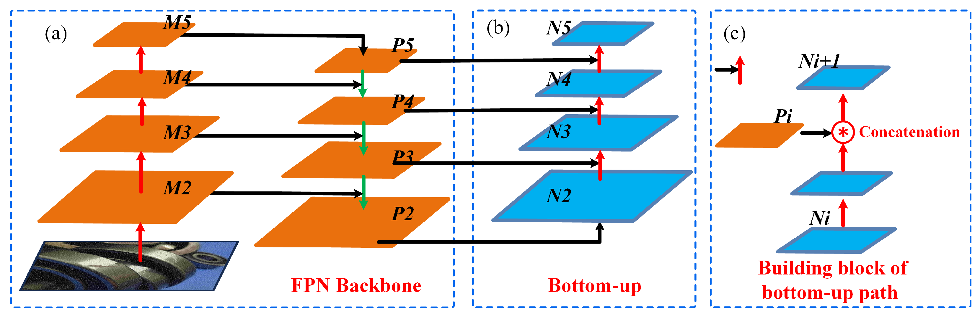
3.3. Neck
3.4. Loss Function
4. Experimental Results and Analysis
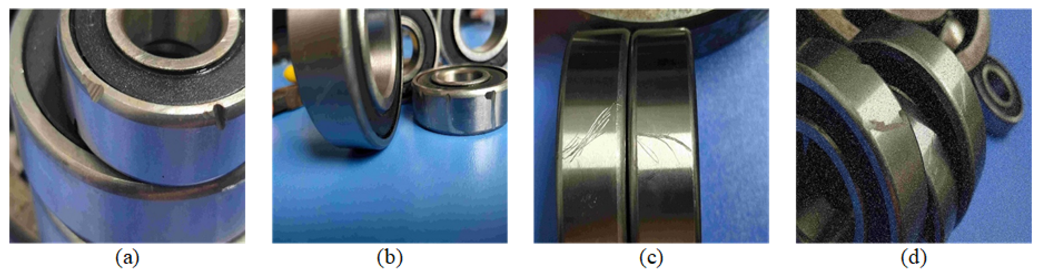
4.1. Dataset Introduction
4.2. Evaluation Metrics
4.3. Experimental Setup
4.4. Analysis of Defect Detection Results
4.4.1. Ablation Experiment
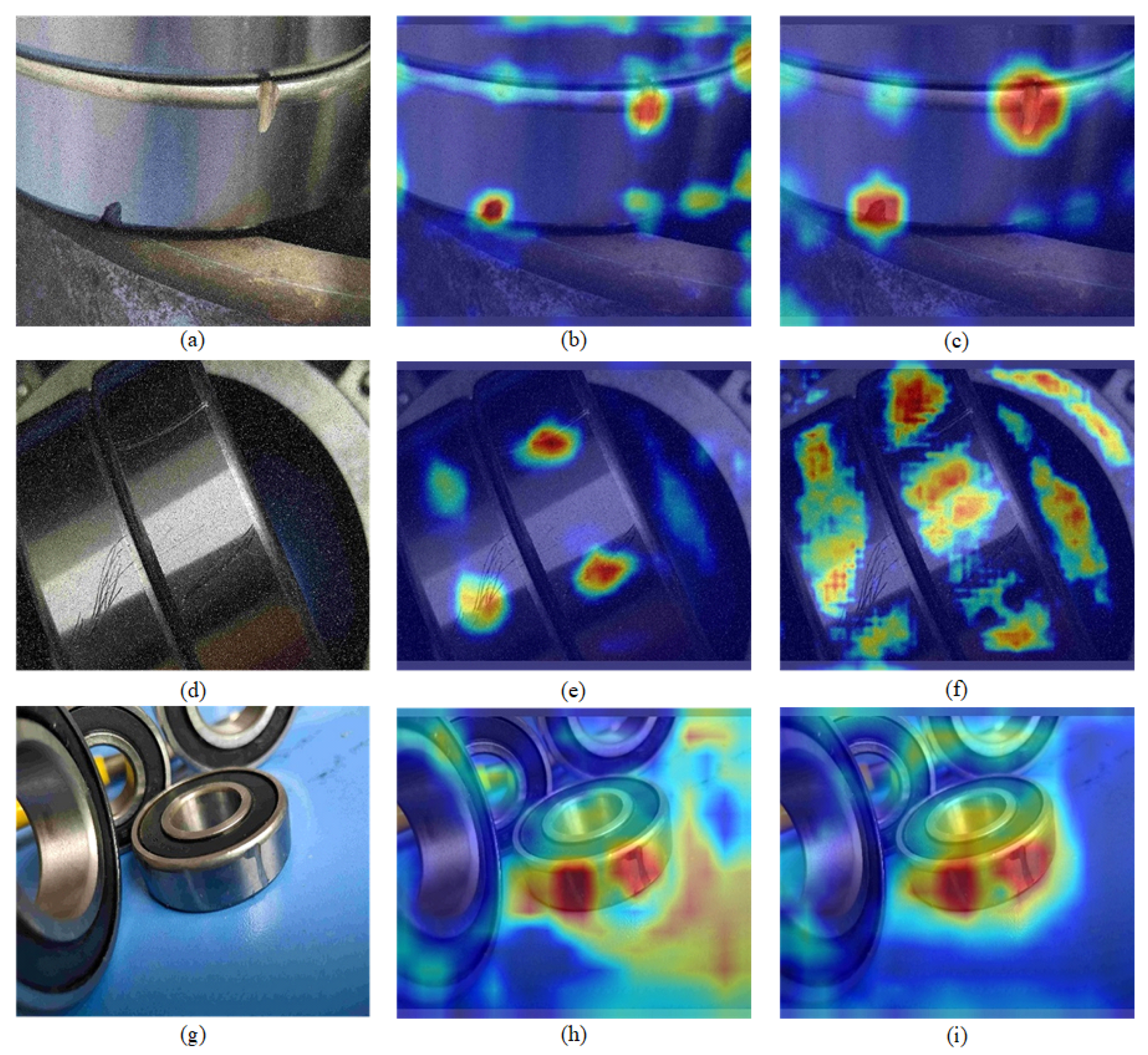
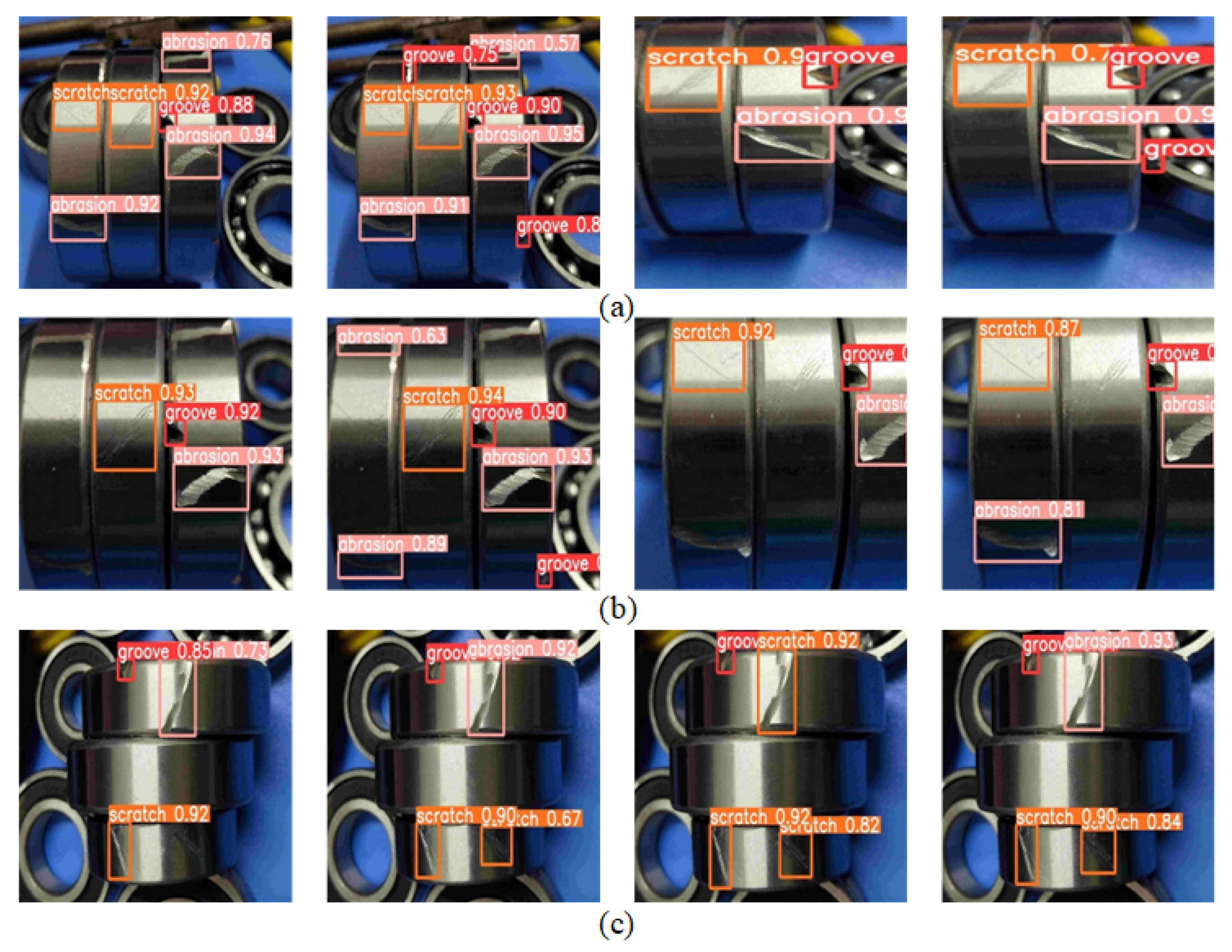
4.4.2. Visualization Result Analysis
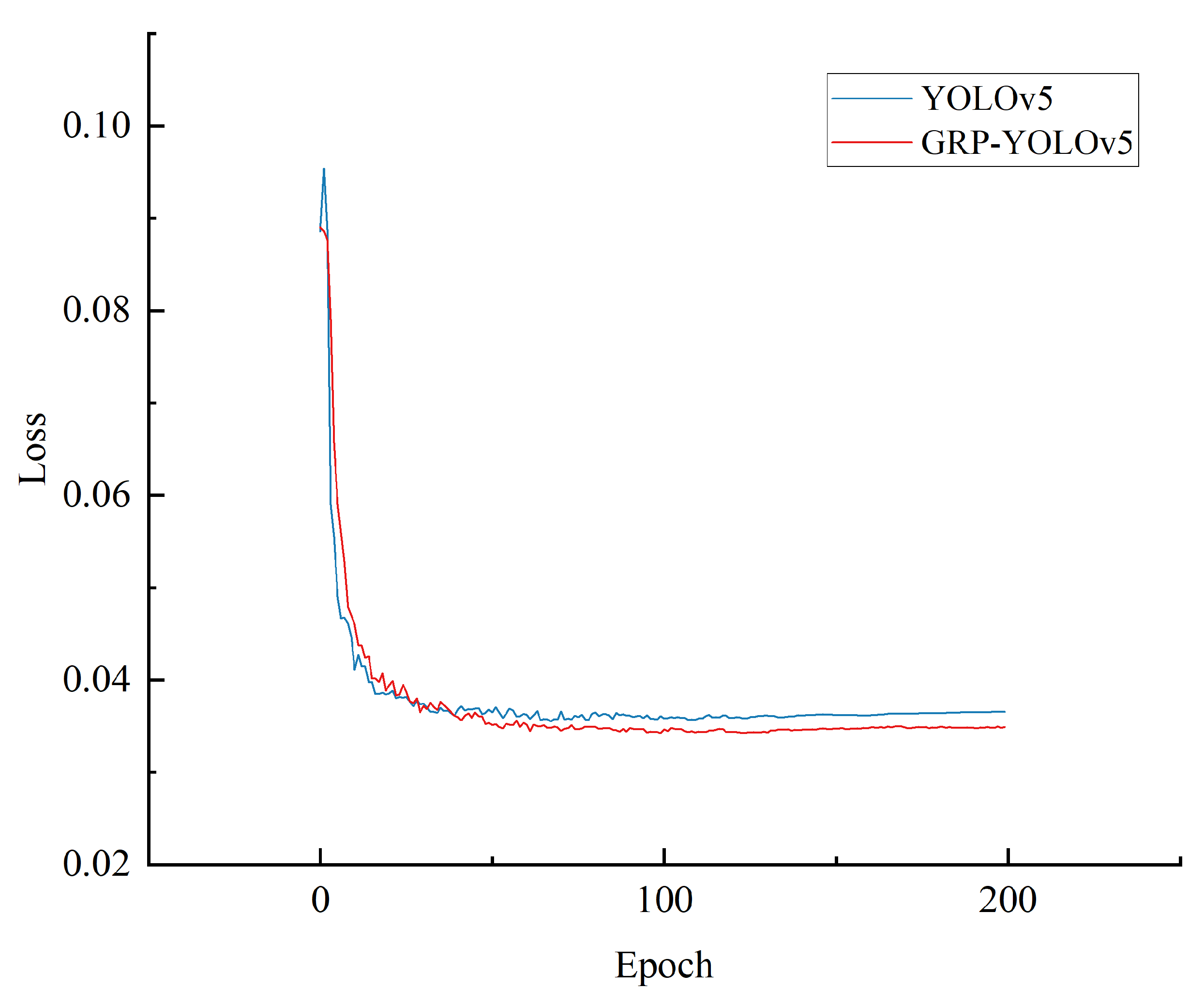
4.4.3. Model Training
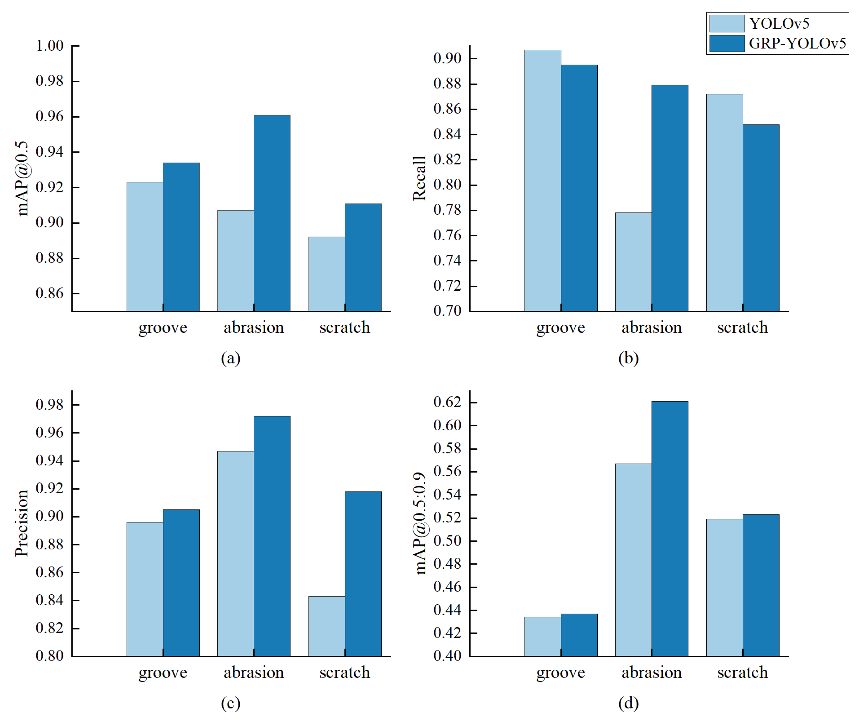
4.4.4. Detection Performance for Different Types of Defects
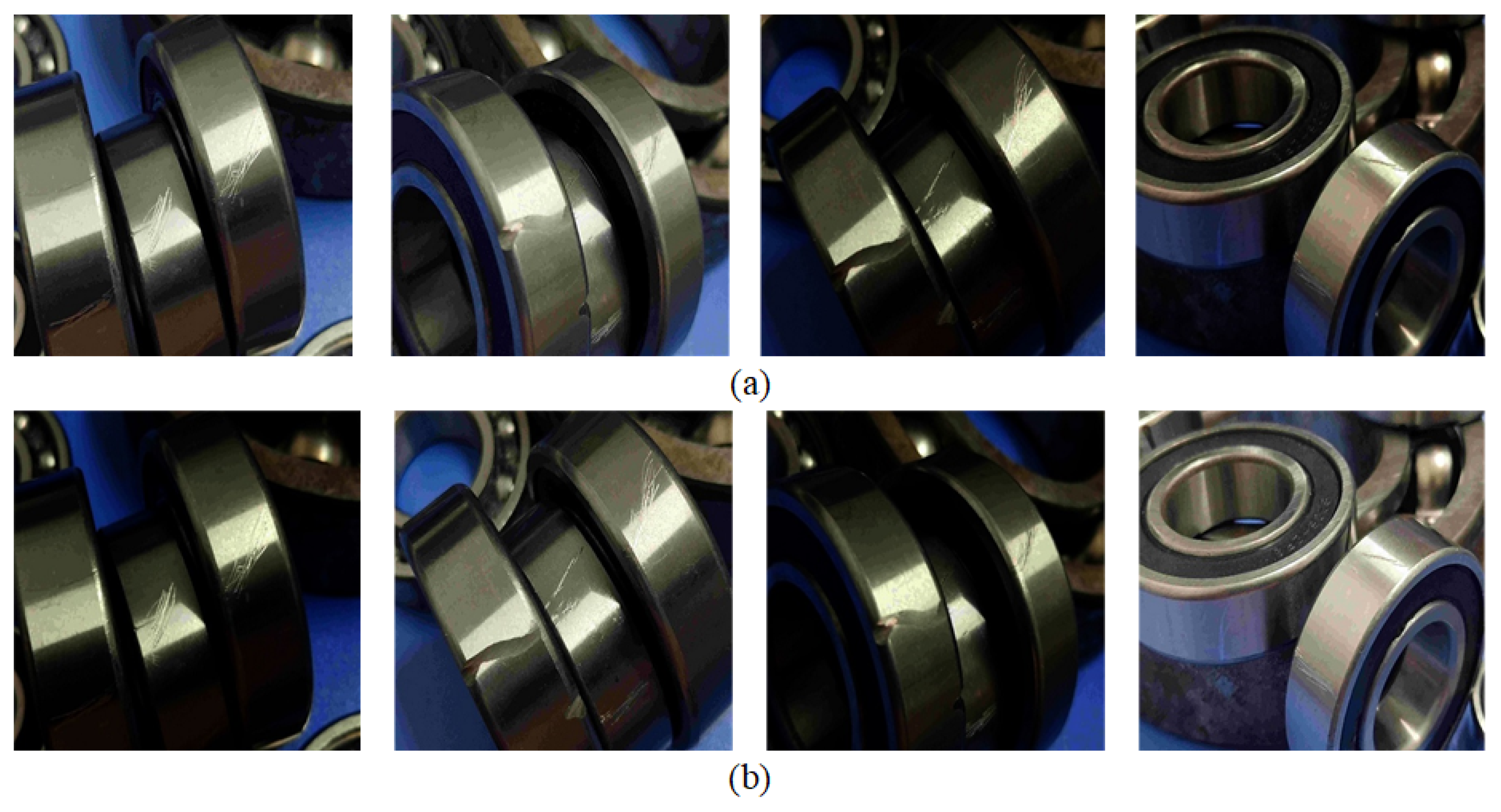
4.4.5. Test Results Visualization
5. Comparative Experiments
6. Conclusions
Author Contributions
Funding
Institutional Review Board Statement
Informed Consent Statement
Data Availability Statement
Acknowledgments
Conflicts of Interest
Sample Availability
References
- Deveci, B.U.; Celtikoglu, M.; Albayrak, O.; Unal, P.; Kirci, P. Transfer Learning Enabled Bearing Fault Detection Methods Based on Image Representations of Single-Dimensional Signals. Inf. Syst. Front. 2023. [Google Scholar] [CrossRef]
- Girshick, R.; Donahue, J.; Darrell, T.; Malik, J. Rich Feature Hierarchies for Accurate Object Detection and Semantic Segmentation. IEEE Comput. Soc. 2014, 8, 580–587. [Google Scholar] [CrossRef]
- Girshick, R.B. Fast R-CNN. In Proceedings of the 2015 IEEE International Conference on Computer Vision (ICCV), Santiago, Chile, 7–13 December 2015; pp. 1440–1448. [Google Scholar]
- Ren, S.; He, K.; Girshick, R.; Sun, J. Faster R-CNN: Towards Real-Time Object Detection with Region Proposal Networks. IEEE Trans. Pattern Anal. Mach. Intell. 2017, 39, 1137–1149. [Google Scholar] [CrossRef] [PubMed]
- Liu, J.; Meng, W. Review on Single-Stage Object Detection Algorithm Based on Deep Learning. Aero Weapon. 2020, 27, 44–53. [Google Scholar]
- Zhao, Y.; Liu, Z.; Yi, D.; Yu, X.; Sha, X.; Li, L.; Sun, H.; Zhan, Z.; Li, W.J. A Review on Rail Defect Detection Systems Based on Wireless Sensors. Sensors 2022, 22, 6409. [Google Scholar] [CrossRef]
- Zhang, X.; Cui, Y.; Wang, Y.; Sun, M.; Hu, H. An improved AE detection method of rail defect based on multi-level ANC with VSS-LMS. Mech. Syst. Signal Process. 2018, 99, 420–433. [Google Scholar] [CrossRef]
- Mandriota, C.; Nitti, M.; Ancona, N.; Stella, E.; Distante, A. Filter-based feature selection for rail defect detection. Mach. Vis. Appl. 2004, 15, 179–185. [Google Scholar] [CrossRef]
- Liu, C.J.; Chen, Z.L.; Liu, P.Y.; Lin, Z.Q. Intelligent bearing quality checking system based on visual inspection. In Proceedings of the 2020 Chinese Automation Congress (CAC), Shanghai, China, 6–8 November 2020. [Google Scholar]
- Pernkopf, F.; O’Leary, P. Visual Inspection of Machined Metallic High-Precision Surfaces. EURASIP J. Adv. Signal Process. 2002, 2002, 650750. [Google Scholar] [CrossRef]
- Ng, T.W. Optical inspection of ball bearing defects. Meas. Sci. Technol. 2007, 18, N73. [Google Scholar] [CrossRef]
- Chen, Y.; Kang, Y.; Feng, B.; Li, Y.; Cai, X.; Wang, S. Automatic defect identification in magnetic particle testing using a digital model aided De-noising method. Measurement 2022, 198, 111427. [Google Scholar] [CrossRef]
- Li, G.P.; Zhang, Y.K.; Ai, C.S.; Ma, Y.Z. Defects Inspection of Steel Ball Based on Optical Fiber Sensing Technique. Appl. Mech. Mater. 2011, 55–57, 658–663. [Google Scholar] [CrossRef]
- Yuzhen, M.; Xuan, S.; Guoping, L.; Xinjua, W. Surface Defect Detection Based on Capacitive Probe for Bearing Ball. In Proceedings of the 2013 25th Chinese Control and Decision Conference (CCDC), Guiyang, China, 25–27 May 2013. [Google Scholar] [CrossRef]
- Esmaeil, M. Modeling and Effect of Ultrasonic Waves on Bearing Shells in Industry by Non-Destructive Testing. Russ. J. Nondestruct. Test. 2020, 56, 853–863. [Google Scholar] [CrossRef]
- Gu, Z.; Liu, X.; Wei, L. A Detection and Identification Method Based on Machine Vision for Bearing Surface Defects. In Proceedings of the 2021 International Conference on Computer, Control and Robotics (ICCCR), Shanghai, China, 8–10 January 2021; pp. 128–132. [Google Scholar]
- Ma, Y.; Ge, X. An Effective Method for Defect Detection of Copper Coated Iron Wire Based on Machine Vision. IOP Conf. Ser. Mater. Sci. Eng. 2019, 631, 022077. [Google Scholar] [CrossRef]
- Liu, G. Surface Defect Detection Methods Based on Deep Learning: A Brief Review. In Proceedings of the 2020 2nd International Conference on Information Technology and Computer Application (ITCA), Guangzhou, China, 18–20 December 2020; pp. 200–203. [Google Scholar]
- Zhao, M.; Song, K.K.; Tian, X.; Liao, X.; Xiao, J. A Method of Removing Oil Droplets from Bearing Image Based on a Two-stage Neural Network. In Proceedings of the 2022 7th International Conference on Signal and Image Processing (ICSIP), Suzhou, China, 20–22 July 2022; pp. 473–479. [Google Scholar]
- Xu, X.J.; Lei, Y.; Yang, F. Railway Subgrade Defect Automatic Recognition Method Based on Improved Faster R-CNN. Sci. Program. 2018, 2018, 4832972. [Google Scholar] [CrossRef]
- Ma, J.; Liu, M.; Hu, S.; Fu, J.; Chen, G.; Yang, A. A novel CNN ensemble framework for bearing surface defects classification based on transfer learning. Meas. Sci. Technol. 2023, 34, 025902. [Google Scholar] [CrossRef]
- Tao, J.; Zhu, Y.; Jiang, F.; Liu, H.; Liu, H. Rolling Surface Defect Inspection for Drum-Shaped Rollers Based on Deep Learning. IEEE Sens. J. 2022, 22, 8693–8700. [Google Scholar] [CrossRef]
- Zheng, Z.; Zhao, J.; Li, Y. Research on Detecting Bearing-Cover Defects Based on Improved YOLOv3. IEEE Access 2021, 9, 10304–10315. [Google Scholar] [CrossRef]
- Song, K.K.; Zhao, M.; Liao, X.; Tian, X.; Zhu, Y.; Xiao, J.; Peng, C. An Improved Bearing Defect Detection Algorithm Based on Yolo. In Proceedings of the 2022 International Symposium on Control Engineering and Robotics (ISCER), Changsha, China, 18–20 February 2022; pp. 184–187. [Google Scholar]
- Wen, S.; Zhou, Z.; Zhang, X.; Chen, Z. Online Detection System of Bearing Roller’s Surface Defects Based on Computational Vision. J. South China Univ. Technol. Nat. Sci. Ed. 2020, 48, 76–87. [Google Scholar]
- Xie, R.; Zhu, Y.; Luo, J.; Qin, G.; Wang, D. Detection algorithm for bearing roller end surface defects based on improved YOLOv5n and image fusion. Meas. Sci. Technol. 2023, 34, 045402. [Google Scholar] [CrossRef]
- Yuan, T.; Yuan, J.; Zhu, Y.; Zheng, H. Surface defect detection algorithm of thrust ball bearing based on improved YOLOv5. J. Zhejiang Univ. Eng. Sci. 2022, 56, 2349–2357. [Google Scholar]
- Yu, G.; Zhou, X. An Improved YOLOv5 Crack Detection Method Combined with a Bottleneck Transformer. Mathematics 2023, 11, 2377. [Google Scholar] [CrossRef]
- Gao, S.H.; Cheng, M.M.; Zhao, K.; Zhang, X.Y.; Yang, M.H.; Torr, P. Res2Net: A New Multi-Scale Backbone Architecture. IEEE Trans. Pattern Anal. Mach. Intell. 2021, 43, 652–662. [Google Scholar] [CrossRef] [PubMed]
- Chen, J.; Kao, S.H.; He, H.; Zhuo, W.; Wen, S.; Lee, C.H.; Chan, S.H.G. Run, Don’t Walk: Chasing Higher FLOPS for Faster Neural Networks. arXiv 2023, arXiv:2303.03667. [Google Scholar]
- Liu, S.; Qi, L.; Qin, H.; Shi, J.; Jia, J. Path Aggregation Network for Instance Segmentation. In Proceedings of the 2018 IEEE/CVF Conference on Computer Vision and Pattern Recognition, Salt Lake City, UT, USA, 16 December 2018; pp. 8759–8768. [Google Scholar] [CrossRef]
- Lin, T.Y.; Dollár, P.; Girshick, R.; He, K.; Hariharan, B.; Belongie, S. Feature Pyramid Networks for Object Detection. In Proceedings of the 2017 IEEE Conference on Computer Vision and Pattern Recognition (CVPR), Honolulu, HI, USA, 21–26 July 2017; pp. 936–944. [Google Scholar] [CrossRef]
- Yadong, L.; Xing, M.; Jiandong, L.; Chunyang, M. Improved Small Target Detection Method of Bearing Defects in YOLOX Network (in Chinese). Comput. Eng. Appl. 2023, 59, 8. [Google Scholar]
- Lin, T.Y.; Goyal, P.; Girshick, R.; He, K.; Dollár, P. Focal Loss for Dense Object Detection. In Proceedings of the 2017 IEEE International Conference on Computer Vision (ICCV), Venice, Italy, 22–29 October 2017; pp. 2999–3007. [Google Scholar] [CrossRef]
- Li, C.; Li, L.; Jiang, H.; Weng, K.; Geng, Y.; Li, L.; Ke, Z.; Li, Q.; Cheng, M.; Nie, W.; et al. YOLOv6: A Single-Stage Object Detection Framework for Industrial Applications. arXiv 2022, arXiv:abs/2209.02976. [Google Scholar]
- Wang, C.Y.; Bochkovskiy, A.; Liao, H.Y.M. YOLOv7: Trainable bag-of-freebies sets new state-of-the-art for real-time object detectors. arXiv 2022, arXiv:abs/2207.02696. [Google Scholar]
- Wei, S.; Jianan, L.I.; Huili, Z.; Yingjiu, H.; Ai, C.S. Research on Surface Defect Detection of Train Bearings Based on Faster R-CNN Algorithm (in Chinese). Mach. Tool Hydraul. 2021, 49, 103–108. [Google Scholar] [CrossRef]
- Ge, Z.; Liu, S.; Wang, F.; Li, Z.; Sun, J. YOLOX: Exceeding YOLO Series in 2021. arXiv 2021, arXiv:abs/2107.08430. [Google Scholar]


| Algorithm | G | R | P | Recall | Precision | mAP@0.5 | mAP@0.5:0.95 | FNR | F-Score |
|---|---|---|---|---|---|---|---|---|---|
| YOLOv5s | 85.2% | 89.5% | 90.7% | 50.6% | 14.8% | 87.3% | |||
| YOLOv5s+G | √ | 86.0% | 89.1% | 91.5% | 50.5% | 14.0% | 87.5% | ||
| YOLOv5s+R | √ | 86.3% | 90.6% | 92.6% | 52.2% | 13.7% | 88.4% | ||
| YOLOv5s+P | √ | 87.1% | 88.3% | 91.6% | 51.4% | 12.9% | 87.7% | ||
| GRP-YOLOv5 | √ | √ | √ | 87.4% | 93.2% | 93.5% | 52.7% | 12.6% | 90.2% |
| Algorithm | mAP@0.5 | mAP@0.5:0.95 | Model Size | GFLOPs | FPS |
|---|---|---|---|---|---|
| SSD | 72.3% | 36.9% | 90.84 MB | 62.7 | 104.8 f/s |
| RetinaNet | 91.9% | 51.4% | 138.16 MB | 146.0 | 26.8 f/s |
| YOLOv6s6 | 88.2% | 48.4% | - | 45.2 | 30.4 f/s |
| YOLOv7 | 93.2% | 52.5% | 141.38 MB | 105.1 | 51.3 f/s |
| YOLOv8s | 90.8% | 52.4% | 42.29 MB | 28.4 | 357.1 f/s |
| YOLOv5s | 90.7% | 50.6% | 26.74 MB | 15.8 | 77.5 f/s |
| Improved Faster R-CNN | 82.2% | 41.2% | 107.55 MB | 941.0 | 18.3 f/s |
| Improved YOLOxs | 89.7% | 51.7% | 33.91 MB | 26.7 | 50.4 f/s |
| GRP-YOLOv5 | 93.5% | 52.7% | 25.17 MB | 16.0 | 68.5 f/s |
Disclaimer/Publisher’s Note: The statements, opinions and data contained in all publications are solely those of the individual author(s) and contributor(s) and not of MDPI and/or the editor(s). MDPI and/or the editor(s) disclaim responsibility for any injury to people or property resulting from any ideas, methods, instructions or products referred to in the content. |
© 2023 by the authors. Licensee MDPI, Basel, Switzerland. This article is an open access article distributed under the terms and conditions of the Creative Commons Attribution (CC BY) license (https://creativecommons.org/licenses/by/4.0/).
Share and Cite
Zhao, Y.; Chen, B.; Liu, B.; Yu, C.; Wang, L.; Wang, S. GRP-YOLOv5: An Improved Bearing Defect Detection Algorithm Based on YOLOv5. Sensors 2023, 23, 7437. https://doi.org/10.3390/s23177437
Zhao Y, Chen B, Liu B, Yu C, Wang L, Wang S. GRP-YOLOv5: An Improved Bearing Defect Detection Algorithm Based on YOLOv5. Sensors. 2023; 23(17):7437. https://doi.org/10.3390/s23177437
Chicago/Turabian StyleZhao, Yue, Bolun Chen, Bushi Liu, Cuiying Yu, Ling Wang, and Shanshan Wang. 2023. "GRP-YOLOv5: An Improved Bearing Defect Detection Algorithm Based on YOLOv5" Sensors 23, no. 17: 7437. https://doi.org/10.3390/s23177437
APA StyleZhao, Y., Chen, B., Liu, B., Yu, C., Wang, L., & Wang, S. (2023). GRP-YOLOv5: An Improved Bearing Defect Detection Algorithm Based on YOLOv5. Sensors, 23(17), 7437. https://doi.org/10.3390/s23177437