

Holistic Spatio-Temporal Graph Attention for Trajectory Prediction in Vehicle–Pedestrian Interactions

Abstract
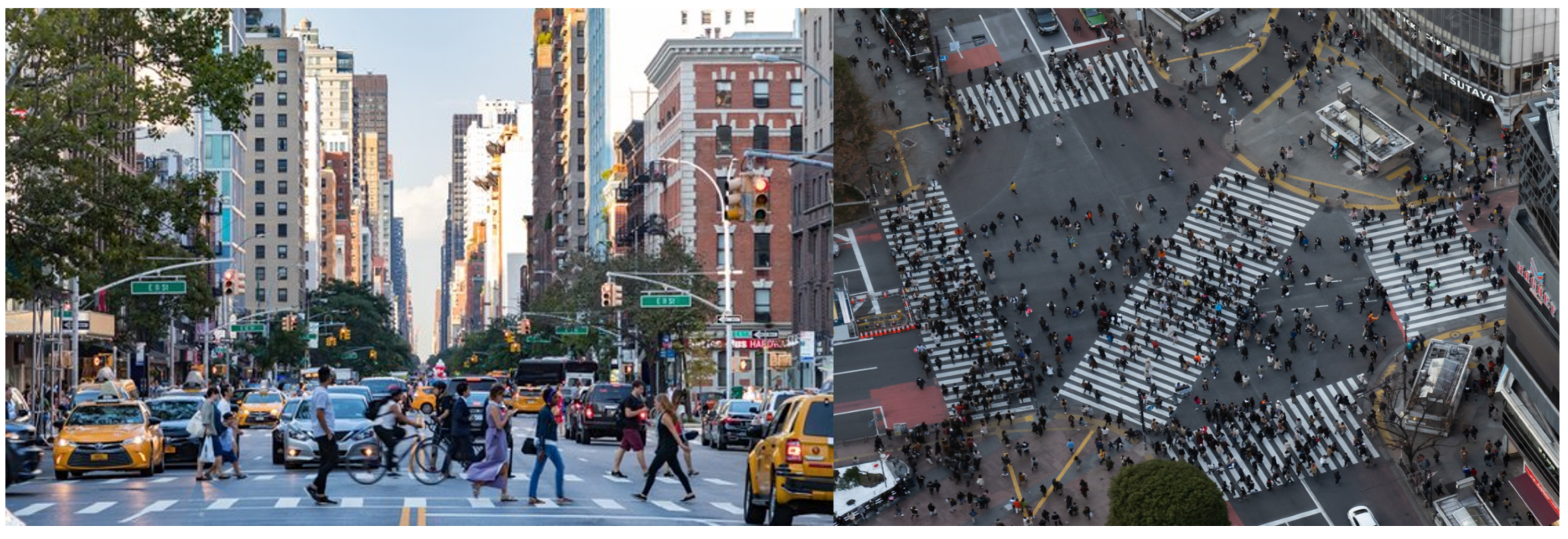
:1. Introduction

- We develop a novel encoder–decoder interaction model called Holistic Spatio-Temporal Graph Attention (HSTGA) for trajectory prediction in vehicle–pedestrian interactions. HSTGA models pedestrian–vehicle interactions in non-signalized and non-crosswalk scenarios using a trajectory-based model for long-horizon pedestrian and vehicle trajectory prediction.
- We develop a vehicle–pedestrian interaction feature extraction model using a multi-layer perceptron (MLP) sub-network and max pooling.
- We develop an LSTM network to adaptively learn the vehicle–pedestrian spatial interaction.
- We predict pedestrian and vehicle trajectories by modeling the spatio-temporal interactions between pedestrian–pedestrian, vehicle–vehicle, and vehicle–pedestrian using only the historical trajectories of pedestrians and vehicles. This approach reduces the information requirements compared to other learning-based methods.
2. Related Works
2.1. Pedestrian Trajectory Prediction Methods
- Physics-based models.
- Planning-based models.
- Pattern-based models.
2.1.1. Physics-Based Models
2.1.2. Planning-Based Models
2.1.3. Pattern-Based Models
2.2. Vehicle–Pedestrian Interaction
2.2.1. Explicit Interaction Modeling
2.2.2. Implicit Interaction Modeling
- Pooling Models
- B.
- Graph Neural Network Model
- C.
- Ego Vehicle–Pedestrian Interaction Model
2.3. Intelligent Vehicle Trajectory Prediction
2.3.1. Interaction-Aware Trajectory Prediction
2.3.2. Graph-Based Interaction Reasoning
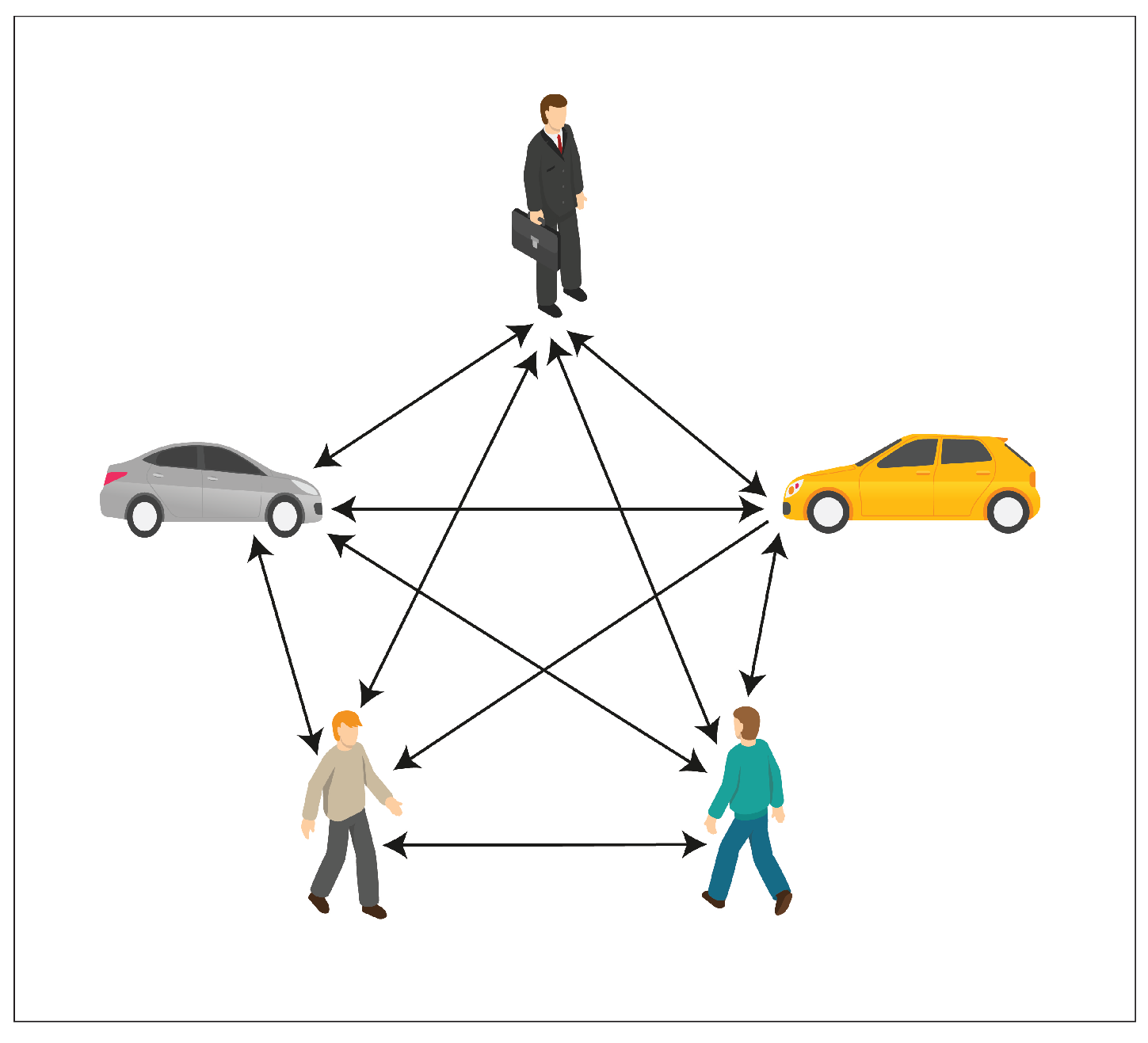
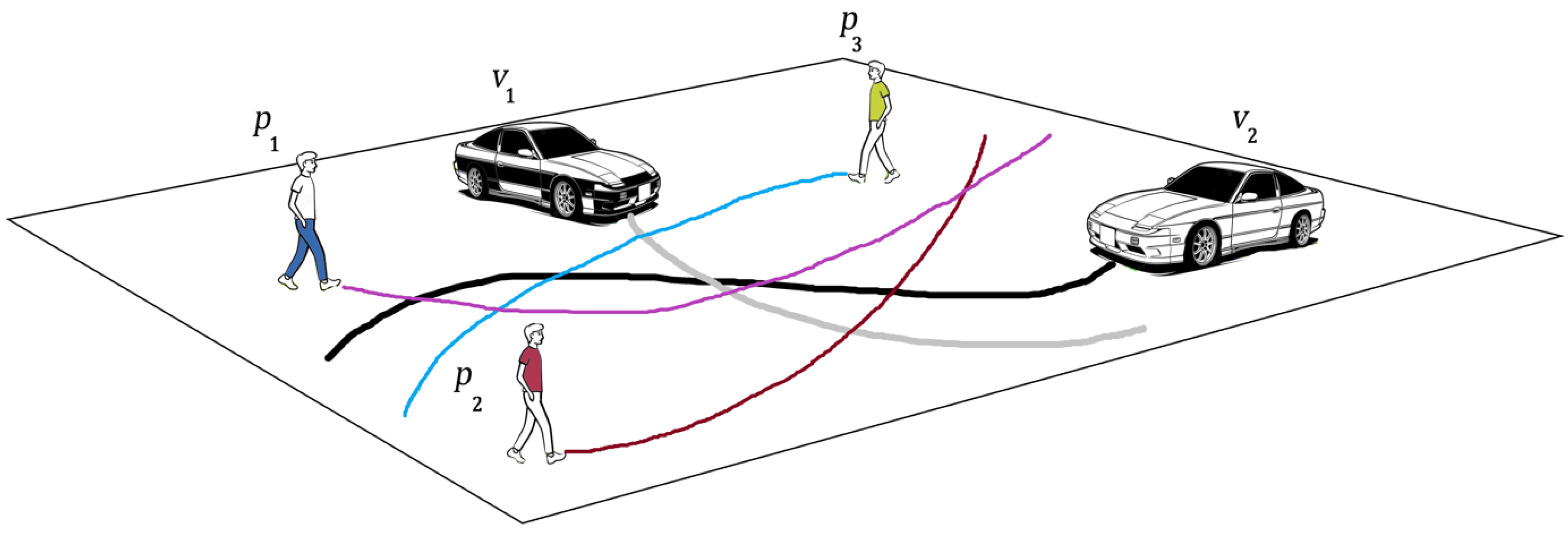
3. Problem Definition
4. Methodology
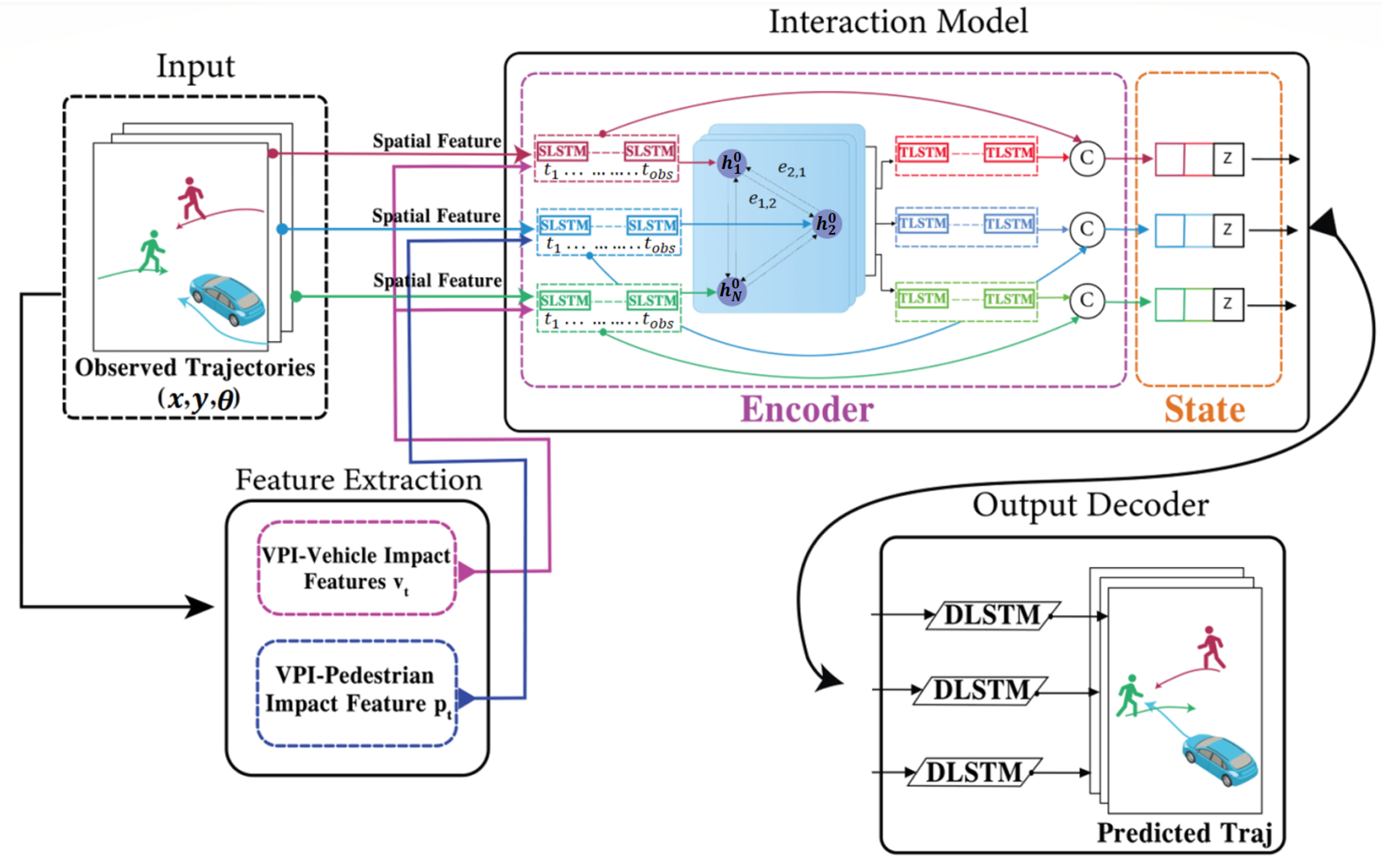
4.1. HSTGA Overview
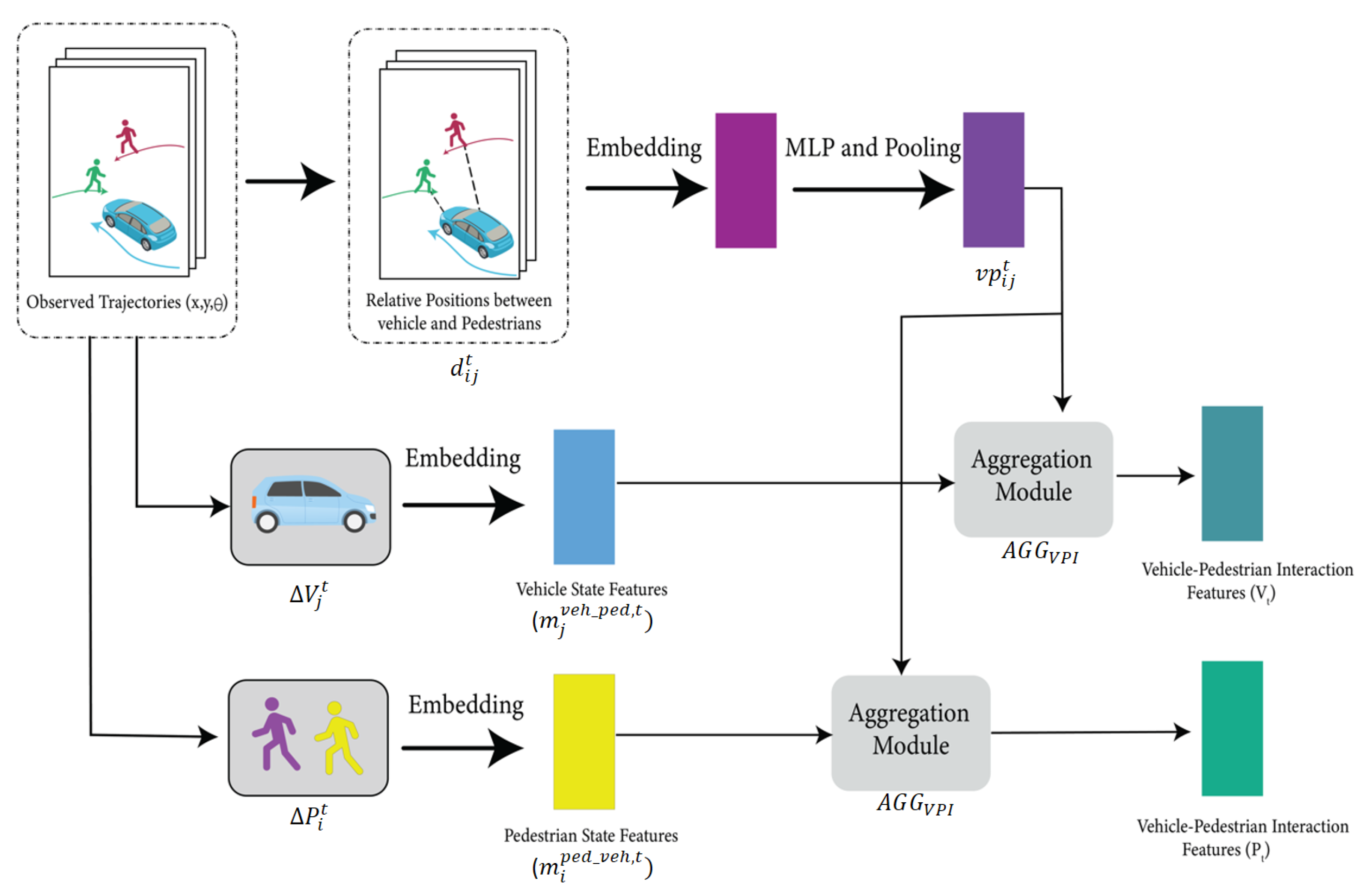
4.2. Vehicle–Pedestrian Interaction (VPI) Feature Extraction
4.3. Trajectory Encoding
4.3.1. Pedestrian Trajectory Encoding
- We first calculate each pedestrian’s relative position and pose to the previous time step.For the relative pose:
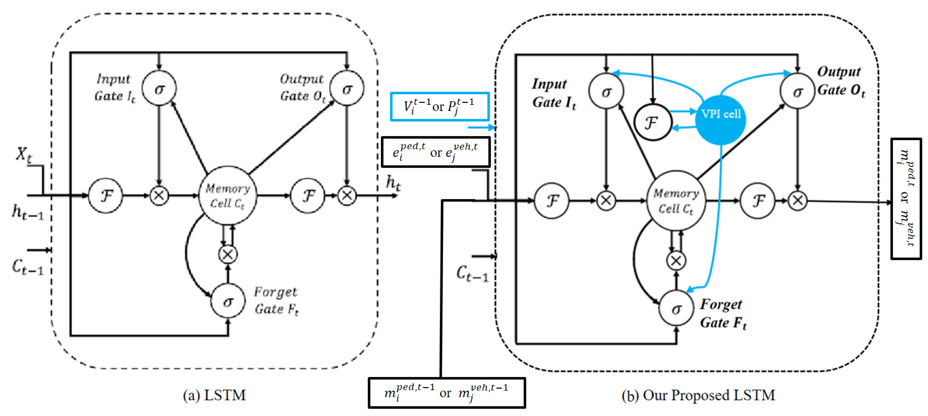
- The calculated relative positions and pose are then embedded into a fixed-length vector for every time step, which is called the spatial feature of the pedestrian.where is an embedding function, and is the embedding weight. This vector is the input to the SLSTM cell. Then, this vector is aggregated with the vehicle–pedestrian interaction feature from Equation (10) and then fed to the SLSTM hidden state.where is the hidden state of the SLSTM at time step t, and is the weight of the SLSTM cell.
4.3.2. Vehicle Trajectory Encoding
- We first calculate each vehicle’s relative position and pose to the previous time step.For the relative pose:
- The calculated relative positions and pose are then embedded into a fixed-length vector for every time step, which is called the spatial feature of the vehicle.where is an embedding function, and is the embedding weight. This vector is the input to the SLSTM cell. Then, this vector is aggregated with the vehicle–pedestrian interaction feature from Equation (11) and then fed to the SLSTM hidden state.where is the hidden state of the SLSTM at time step t, and is the weight of the SLSTM cell.
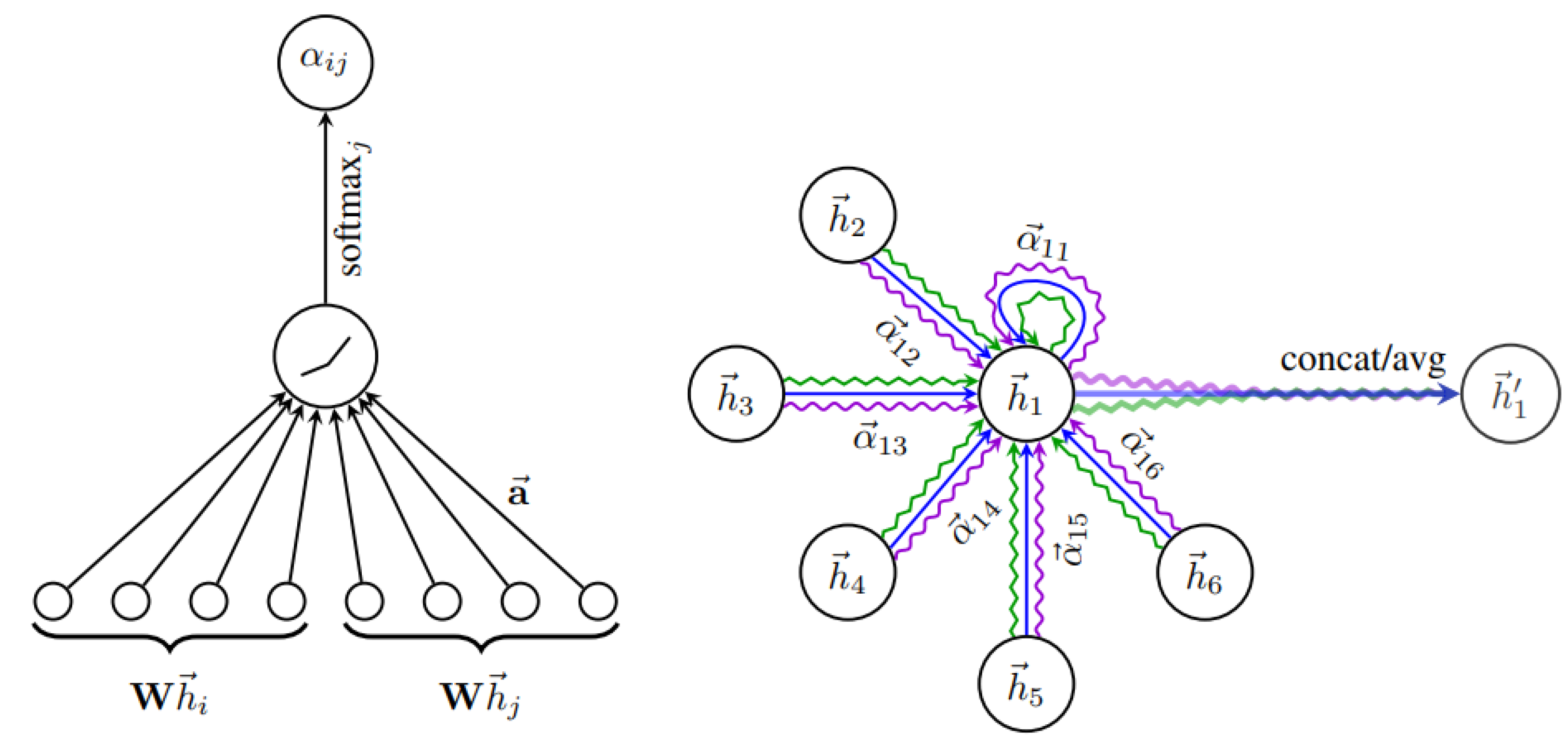
4.4. Interaction Modeling and Prediction
5. Implementation Details
- The variety loss is selected, as shown in Equations (39) and (40), to quantify the difference between the predicted and actual trajectories. Moreover, we used two evaluation metrics, namely the Average Displacement Error (ADE) and Final Displacement Error (FDE), to report the prediction errors.
- The Adam optimizer is used with a good learning rate to balance fast convergence and avoid overshooting.
- Batch-size, backpropagation, weight-update, and regularization techniques are included in our model implementation.
- Proper datasets for training and validation are an essential part of our model implementation.
- We monitor the performance of our model and tune the hyperparameters if needed.
6. Experiments
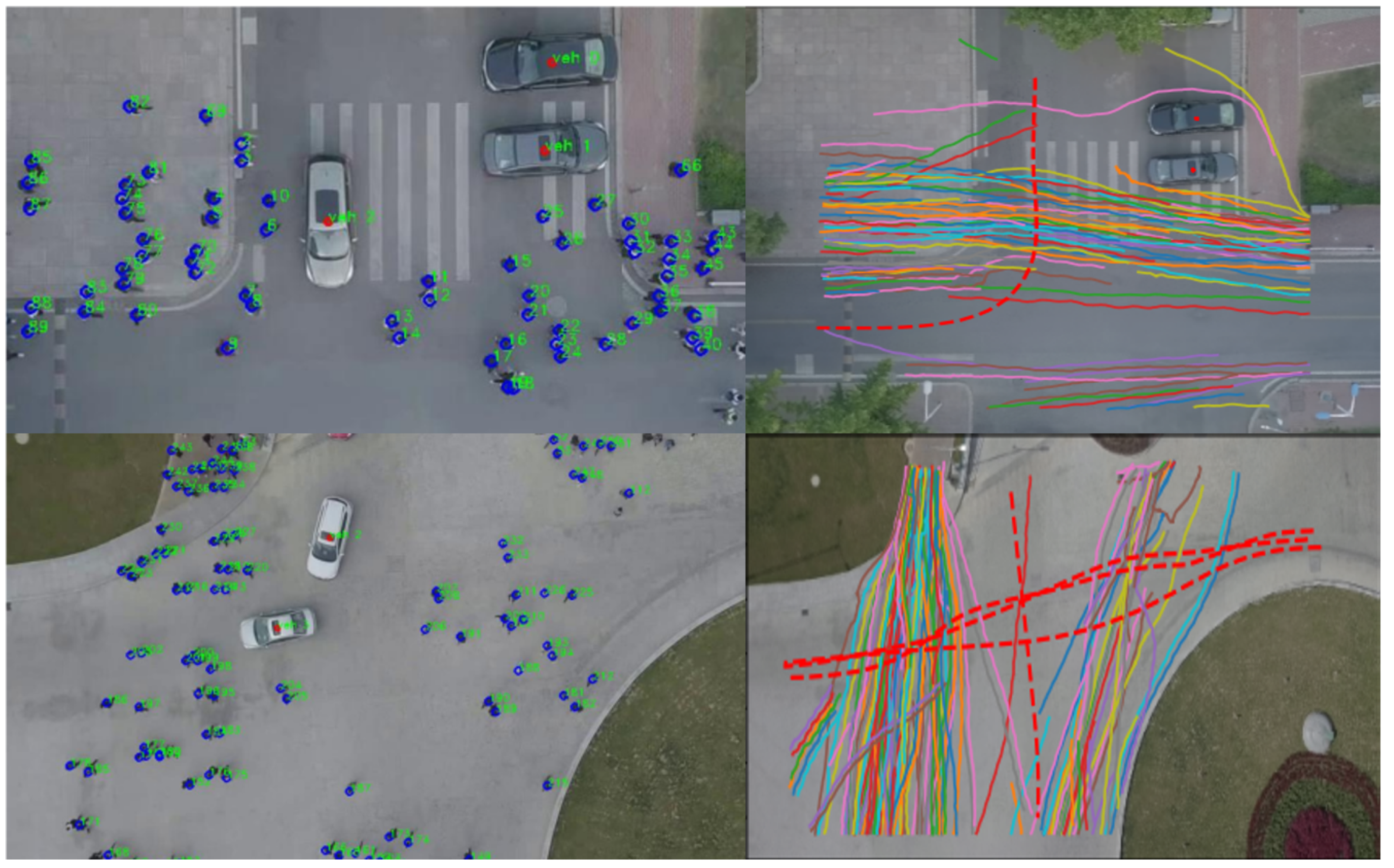
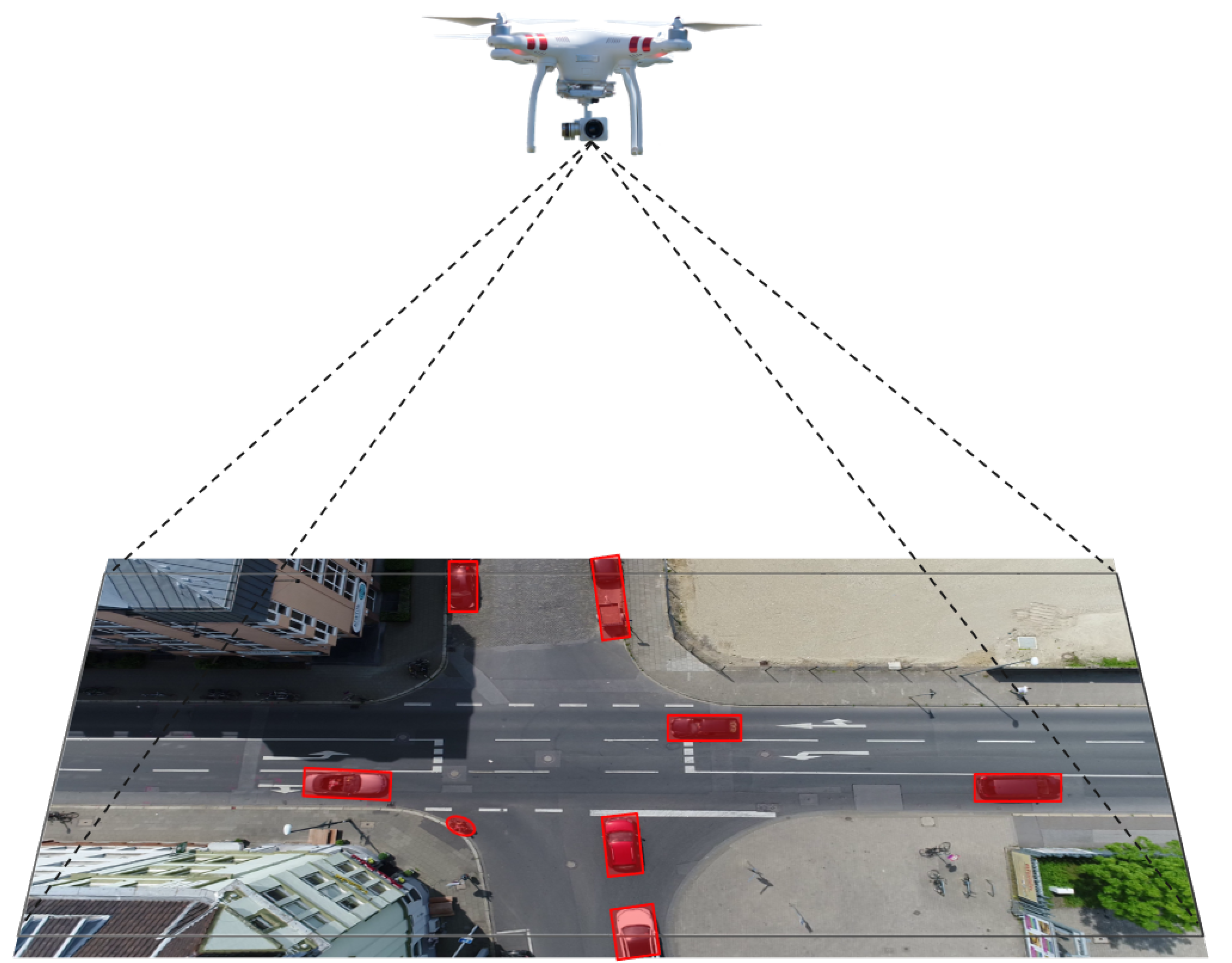
6.1. Dataset
6.2. Evaluation Metrics
- Average Displacement Error (ADE): The mean distance between the actual and predicted trajectories over all predicted time steps, as specified in Equation (40).
- Final Displacement Error (FDE): The mean distance between the actual and predicted trajectories at the last predicted time step, which is expressed in Equation (41).
7. Results and Analysis
7.1. Quantitative Results
- Constant Velocity (CV) [79]: The pedestrian is assumed to travel at a constant velocity.
- Social GAN (SGAN) [52]: A GAN architecture that uses a permutation-invariant pooling module to capture pedestrian interactions at different scales.
- Multi-Agent Tensor Fusion (MATF) [54]: A GAN architecture that uses a global pooling layer to combine trajectory and semantic information.
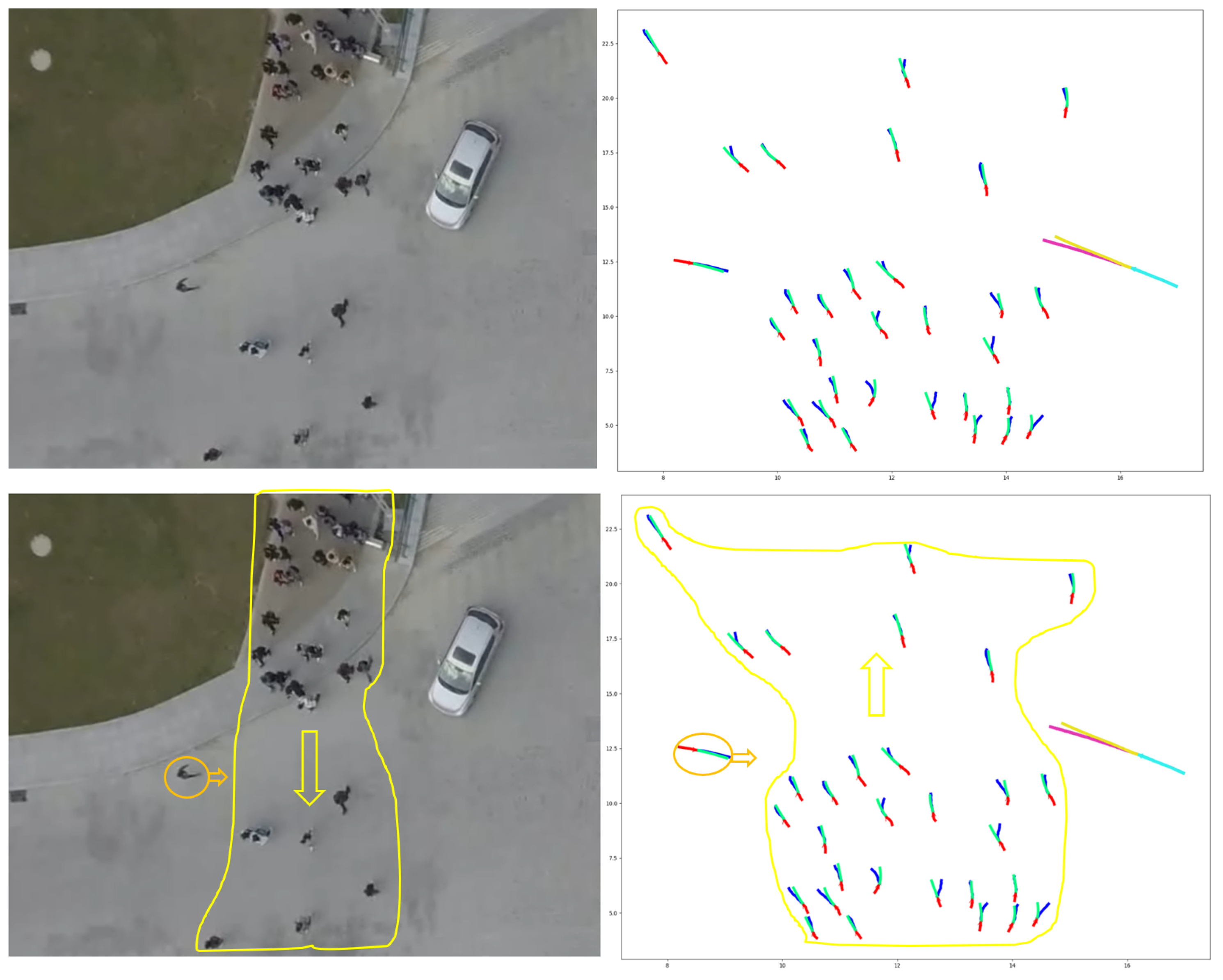
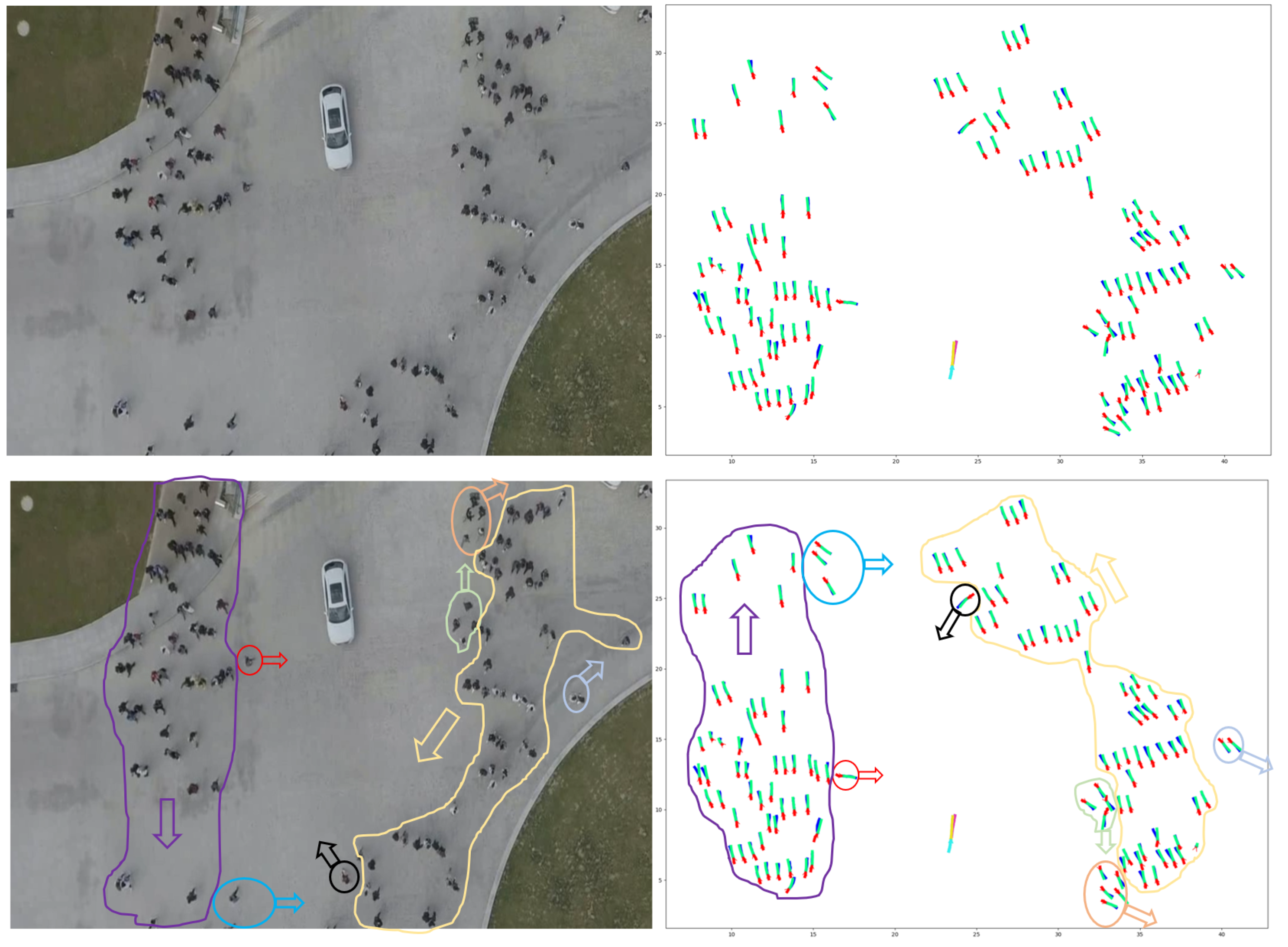
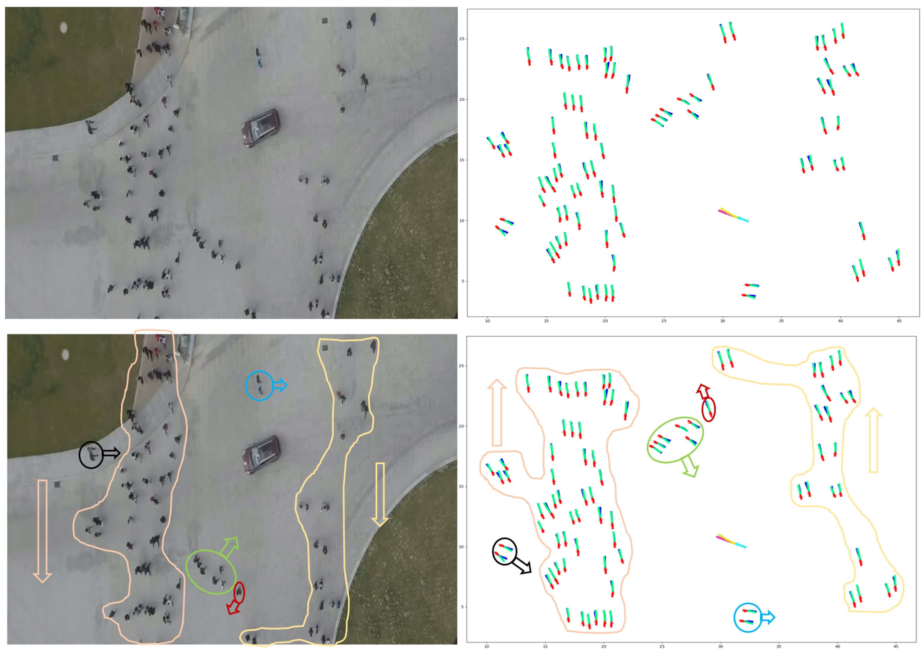
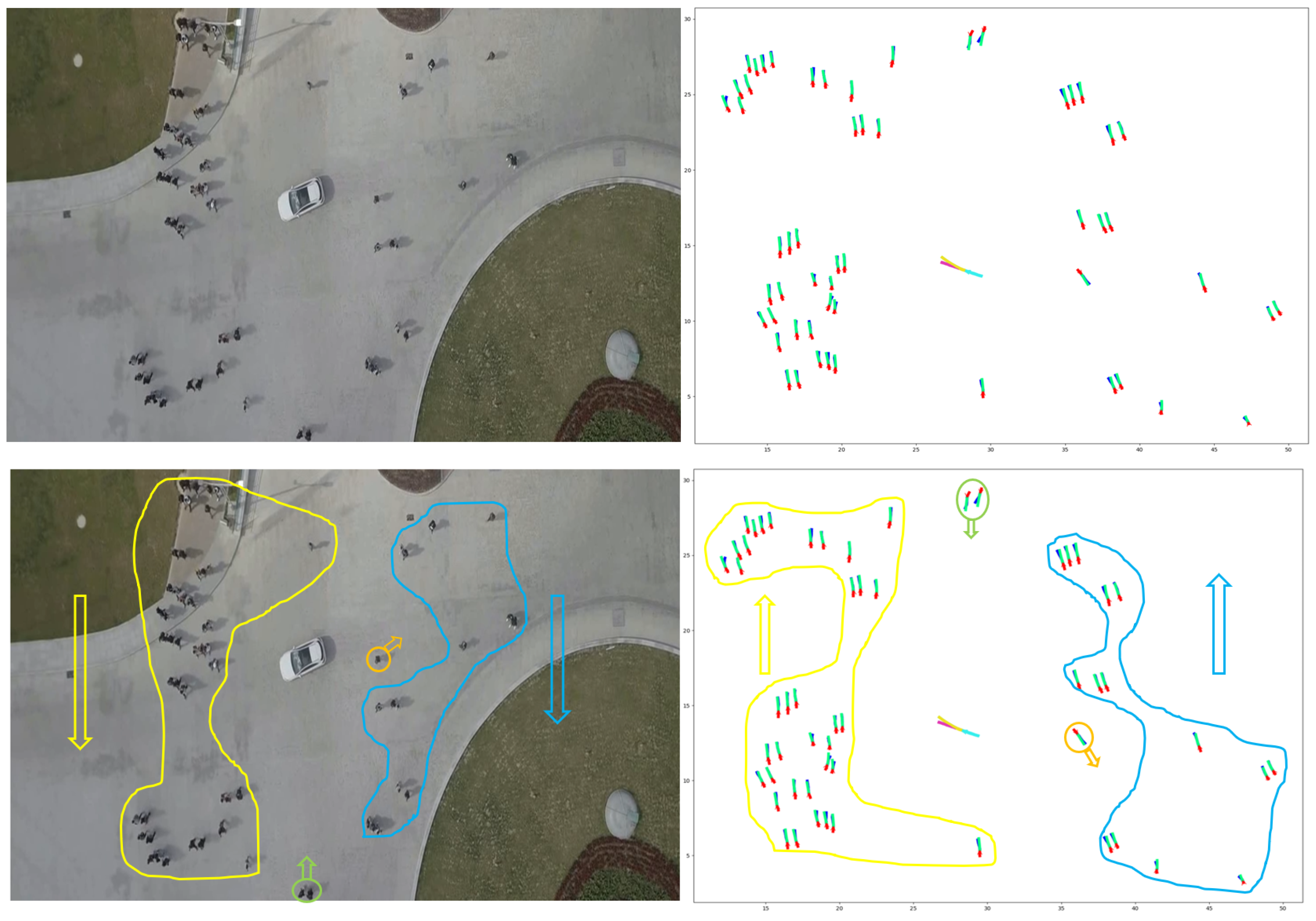
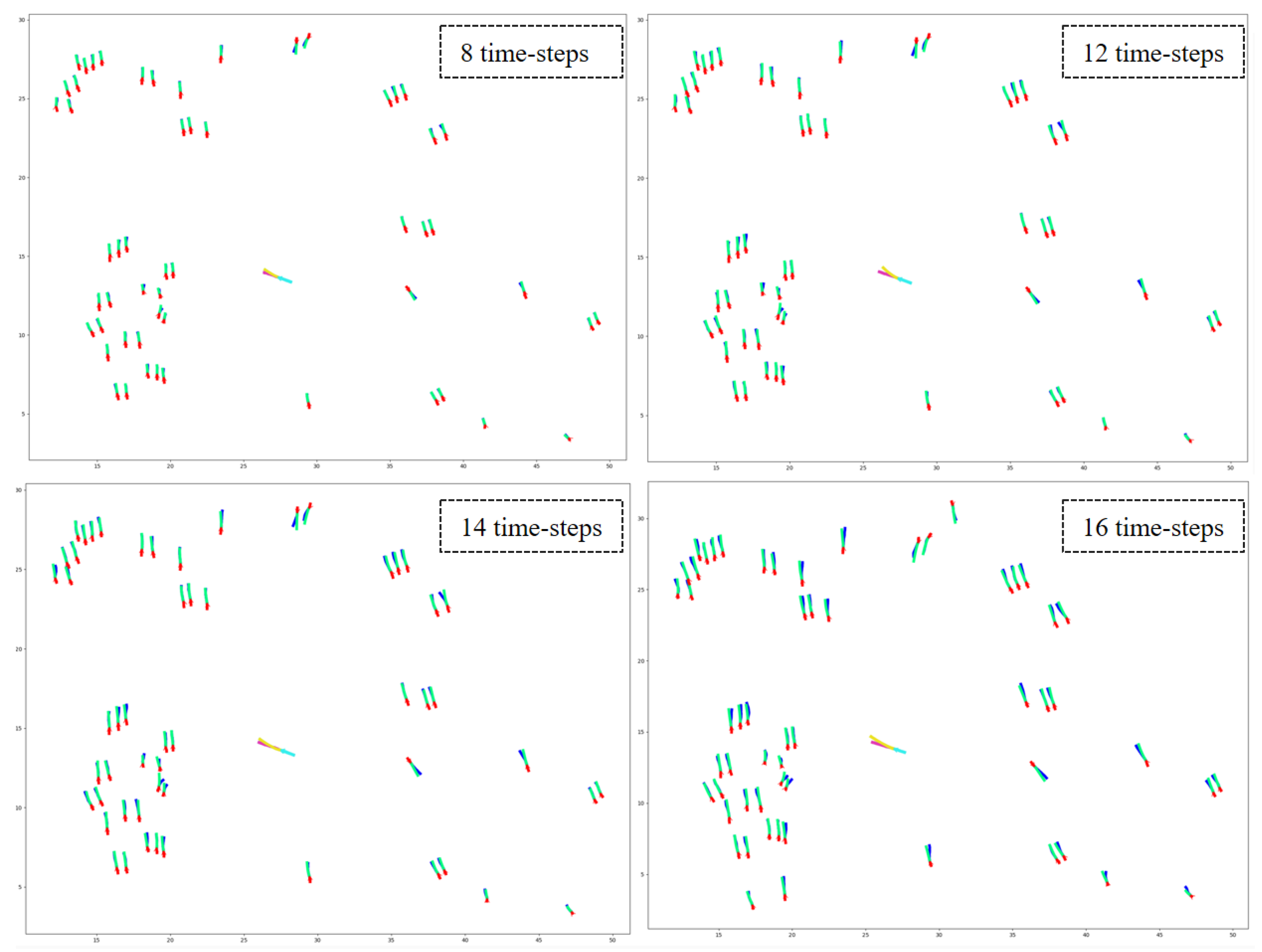
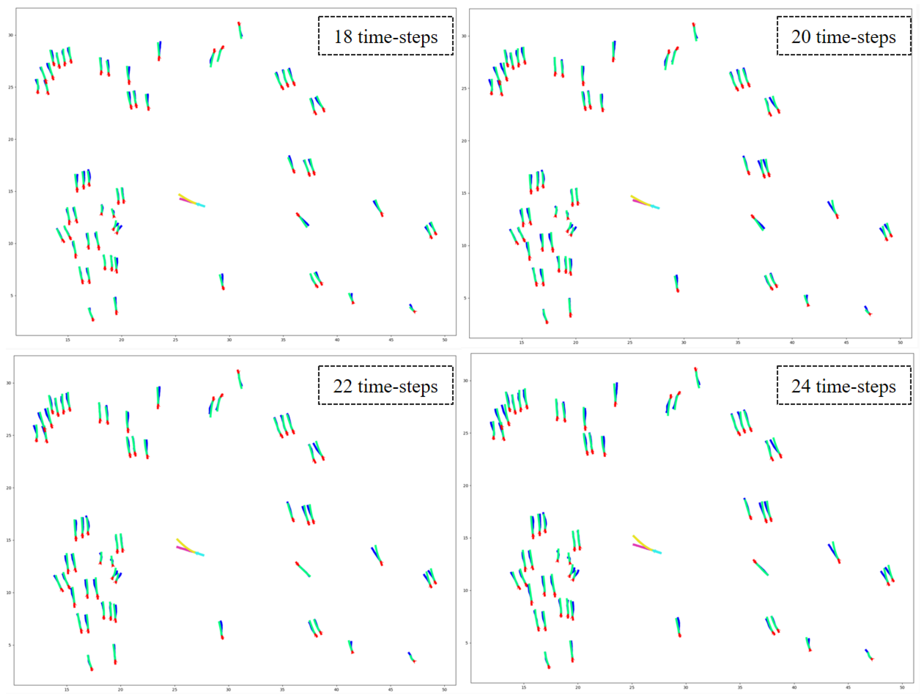
7.2. Qualitative Results
8. Conclusions
Author Contributions
Funding
Institutional Review Board Statement
Informed Consent Statement
Data Availability Statement
Conflicts of Interest
References
- Pedestrian Safety | NHTSA. Available online: https://www.nhtsa.gov/road-safety/pedestrian-safety (accessed on 6 April 2023).
- Seize the Moment to Tackle Road Crash Deaths and Build a Safe and Sustainable Future. Available online: https://www.who.int/news/item/25-06-2023-seize-the-moment-to-tackle-road-crash-deaths-and-build-a-safe-and-sustainable-future (accessed on 14 August 2023).
- Ahmed, S.K.; Mohammed, M.G.; Abdulqadir, S.O.; El-Kader, R.G.A.; El-Shall, N.A.; Chandran, D.; Rehman, M.E.U.; Dhama, K. Road traffic accidental injuries and deaths: A neglected global health issue. Health Sci. Rep. 2023, 6, e1240. [Google Scholar] [CrossRef] [PubMed]
- Pedestrian Safety Campaign. Available online: http://txdot.gov/en/home/safety/traffic-safety-campaigns/pedestrian-safety.html (accessed on 16 April 2023).
- Lu, Y.; Shen, J.; Wang, C.; Lu, H.; Xin, J. Studying on the design and simulation of collision protection system between vehicle and pedestrian. Int. J. Distrib. Sens. Netw. 2020, 16, 1550147719900109. [Google Scholar] [CrossRef]
- Crandall, J.R.; Bhalla, K.S.; Madeley, N.J. Designing road vehicles for pedestrian protection. BMJ 2002, 324, 1145–1148. [Google Scholar] [CrossRef]
- Stcherbatcheff, G.; Tarriere, C.; Duclos, P.; Fayon, A.; Got, C.; Patel, A. Simulation of Collisions Between Pedestrians and Vehicles Using Adult and Child Dummies; SAE Technical Paper 751167; SAE International: Warrendale, PA, USA, 1975. [Google Scholar] [CrossRef]
- Ganichev, A.; Batishcheva, O. Evaluating the conflicts between vehicles and pedestrians. Transp. Res. Procedia 2020, 50, 145–151. [Google Scholar] [CrossRef]
- Tahmasbi-Sarvestani, A.; Mahjoub, H.N.; Fallah, Y.P.; Moradi-Pari, E.; Abuchaar, O. Implementation and Evaluation of a Cooperative Vehicle-to-Pedestrian Safety Application. IEEE Intell. Transp. Syst. Mag. 2017, 9, 62–75. [Google Scholar] [CrossRef]
- Gandhi, T.; Trivedi, M.M. Pedestrian Protection Systems: Issues, Survey, and Challenges. IEEE Trans. Intell. Transp. Syst. 2007, 8, 413–430. [Google Scholar] [CrossRef]
- Amini, R.E.; Yang, K.; Antoniou, C. Development of a conflict risk evaluation model to assess pedestrian safety in interaction with vehicles. Accid. Anal. Prev. 2022, 175, 106773. [Google Scholar] [CrossRef]
- Bai, S.; Legge, D.D.; Young, A.; Bao, S.; Zhou, F. Investigating External Interaction Modality and Design Between Automated Vehicles and Pedestrians at Crossings. In Proceedings of the 2021 IEEE International Intelligent Transportation Systems Conference (ITSC), Indianapolis, IN, USA, 19–22 September 2021; pp. 1691–1696. [Google Scholar] [CrossRef]
- Plitt, A. New York City’s Streets Are ‘More Congested Than Ever’: Report. Curbed NY, 15 August 2019. Available online: https://ny.curbed.com/2019/8/15/20807470/nyc-streets-dot-mobility-report-congestion (accessed on 6 May 2023).
- Pedestrian Scramble. Wikipedia. 2 May 2023. Available online: https://en.wikipedia.org/w/index.php?title=Pedestrian_scramble&oldid=1152818953 (accessed on 6 May 2023).
- Zheng, L.; Ismail, K.; Meng, X. Traffic conflict techniques for road safety analysis: Open questions and some insights. Can. J. Civ. Eng. 2014, 41, 633–641. [Google Scholar] [CrossRef]
- Parker, M.R. Traffic Conflict Techniques for Safety and Operations: Observers Manual; Federal Highway Administration: McLean, VA, USA, 1989.
- Amundsen and Hydén. In Proceedings of the 1st Workshop on Traffic Conflicts, Oslo, Norway, November 1977.
- Almodfer, R.; Xiong, S.; Fang, Z.; Kong, X.; Zheng, S. Quantitative analysis of lane-based pedestrian-vehicle conflict at a non-signalized marked crosswalk. Transp. Res. Part F Traffic Psychol. Behav. 2016, 42, 468–478. [Google Scholar] [CrossRef]
- Liu, Y.-C.; Tung, Y.-C. Risk analysis of pedestrians’ road-crossing decisions: Effects of age, time gap, time of day, and vehicle speed. Saf. Sci. 2014, 63, 77–82. [Google Scholar] [CrossRef]
- Yagil, D. Beliefs, motives and situational factors related to pedestrians’ self-reported behavior at signal-controlled crossings. Transp. Res. Part F Traffic Psychol. Behav. 2000, 3, 1–13. [Google Scholar] [CrossRef]
- Tom, A.; Granié, M.-A. Gender differences in pedestrian rule compliance and visual search at signalized and unsignalized crossroads. Accid. Anal. Prev. 2011, 43, 1794–1801. [Google Scholar] [CrossRef] [PubMed]
- Cheng, G.; Wang, Y.; Li, D. Setting Conditions of Crosswalk Signal on Urban Road Sections in China. ScholarMate. 2013. Available online: https://www.scholarmate.com/A/Evu6ja (accessed on 18 April 2023).
- Himanen, V.; Kulmala, R. An application of logit models in analysing the behaviour of pedestrians and car drivers on pedestrian crossings. Accid. Anal. Prev. 1988, 20, 187–197. [Google Scholar] [CrossRef] [PubMed]
- Shetty, A.; Yu, M.; Kurzhanskiy, A.; Grembek, O.; Tavafoghi, H.; Varaiya, P. Safety challenges for autonomous vehicles in the absence of connectivity. Transp. Res. Part C Emerg. Technol. 2021, 128, 103133. [Google Scholar] [CrossRef]
- Iftikhar, S.; Zhang, Z.; Asim, M.; Muthanna, A.; Koucheryavy, A.; El-Latif, A.A.A. Deep Learning-Based Pedestrian Detection in Autonomous Vehicles: Substantial Issues and Challenges. Electronics 2022, 11, 21. [Google Scholar] [CrossRef]
- Eiffert, S.; Li, K.; Shan, M.; Worrall, S.; Sukkarieh, S.; Nebot, E. Probabilistic Crowd GAN: Multimodal Pedestrian Trajectory Prediction using a Graph Vehicle-Pedestrian Attention Network. IEEE Robot. Autom. Lett. 2020, 5, 5026–5033. [Google Scholar] [CrossRef]
- Chandra, R.; Bhattacharya, U.; Bera, A.; Manocha, D. TraPHic: Trajectory Prediction in Dense and Heterogeneous Traffic Using Weighted Interactions. In Proceedings of the 2019 IEEE/CVF Conference on Computer Vision and Pattern Recognition (CVPR), Long Beach, CA, USA, 15–20 June 2019; pp. 8475–8484. [Google Scholar] [CrossRef]
- Chandra, R.; Bhattacharya, U.; Roncal, C.; Bera, A.; Manocha, D. RobustTP: End-to-End Trajectory Prediction for Heterogeneous Road-Agents in Dense Traffic with Noisy Sensor Inputs. arXiv 2019, arXiv:1907.08752. [Google Scholar]
- Chandra, R.; Guan, T.; Panuganti, S.; Mittal, T.; Bhattacharya, U.; Bera, A.; Manocha, D. Forecasting Trajectory and Behavior of Road-Agents Using Spectral Clustering in Graph-LSTMs. arXiv 2020, arXiv:1912.01118. [Google Scholar] [CrossRef]
- Carrasco, S.; Llorca, D.F.; Sotelo, M.Á. SCOUT: Socially-COnsistent and UndersTandable Graph Attention Network for Trajectory Prediction of Vehicles and VRUs. arXiv 2021, arXiv:2102.06361. [Google Scholar]
- Pellegrini, S.; Ess, A.; Schindler, K.; van Gool, L. You’ll never walk alone: Modeling social behavior for multi-target tracking. In Proceedings of the 2009 IEEE 12th International Conference on Computer Vision, Kyoto, Japan, 29 September–2 October 2009; pp. 261–268. [Google Scholar] [CrossRef]
- Lerner, A.; Chrysanthou, Y.; Lischinski, D. Crowds by Example. Comput. Graph. Forum 2007, 26, 655–664. [Google Scholar] [CrossRef]
- Yang, D.; Li, L.; Redmill, K.; Özgüner, Ü. Top-view Trajectories: A Pedestrian Dataset of Vehicle-Crowd Interaction from Controlled Experiments and Crowded Campus. arXiv 2019, arXiv:1902.00487. [Google Scholar]
- Krajewski, R.; Moers, T.; Bock, J.; Vater, L.; Eckstein, L. The rounD Dataset: A Drone Dataset of Road User Trajectories at Roundabouts in Germany. In Proceedings of the 2020 IEEE 23rd International Conference on Intelligent Transportation Systems (ITSC), Rhodes, Greece, 20–23 September 2020; pp. 1–6. [Google Scholar] [CrossRef]
- Bock, J.; Vater, L.; Krajewski, R.; Moers, T. Highly Accurate Scenario and Reference Data for Automated Driving. ATZ Worldw 2021, 123, 50–55. [Google Scholar] [CrossRef]
- Rudenko, A.; Palmieri, L.; Herman, M.; Kitani, K.M.; Gavrila, D.M.; Arras, K.O. Human Motion Trajectory Prediction: A Survey. Int. J. Robot. Res. 2020, 39, 895–935. [Google Scholar] [CrossRef]
- Zhang, E.; Masoud, N.; Bandegi, M.; Lull, J.; Malhan, R.K. Step Attention: Sequential Pedestrian Trajectory Prediction. IEEE Sensors J. 2022, 22, 8071–8083. [Google Scholar] [CrossRef]
- Kim, S.; Guy, S.J.; Liu, W.; Wilkie, D.; Lau, R.W.H.; Lin, M.C.; Manocha, D. BRVO: Predicting pedestrian trajectories using velocity-space reasoning. Int. J. Robot. Res. 2015, 34, 201–217. [Google Scholar] [CrossRef]
- Zanlungo, F.; Ikeda, T.; Kanda, T. Social force model with explicit collision prediction. EPL 2011, 93, 68005. [Google Scholar] [CrossRef]
- Martinelli, A.; Gao, H.; Groves, P.D.; Morosi, S. Probabilistic Context-Aware Step Length Estimation for Pedestrian Dead Reckoning. IEEE Sensors J. 2018, 18, 1600–1611. [Google Scholar] [CrossRef]
- SmartPDR: Smartphone-Based Pedestrian Dead Reckoning for Indoor Localization. IEEE Sens. J. 2015, 15, 15018804. Available online: https://ieeexplore.ieee.org/document/6987239 (accessed on 5 May 2023).
- Indoor Trajectory Prediction Algorithm Based on Communication Analysis of Built-In Sensors in Mobile Terminals. IEEE Sens. J. 2021, 21, 21388524.
- Ziebart, B.D.; Ratliff, N.; Gallagher, G.; Mertz, C.; Peterson, K.; Bagnell, J.A.; Hebert, M.; Dey, A.K.; Srinivasa, S. Planning-based prediction for pedestrians. In Proceedings of the 2009 IEEE/RSJ International Conference on Intelligent Robots and Systems, St. Louis, MO, USA, 10–15 October 2009; pp. 3931–3936. [Google Scholar] [CrossRef]
- Galata, A.; Johnson, N.; Hogg, D. Learning Variable-Length Markov Models of Behavior. Comput. Vis. Image Underst. 2001, 81, 398–413. [Google Scholar] [CrossRef]
- Deo, N.; Trivedi, M.M. Learning and predicting on-road pedestrian behavior around vehicles. In Proceedings of the 2017 IEEE 20th International Conference on Intelligent Transportation Systems (ITSC), Yokohama, Japan, 16–19 October 2017; pp. 1–6. [Google Scholar] [CrossRef]
- Rehder, E.; Wirth, F.; Lauer, M.; Stiller, C. Pedestrian Prediction by Planning Using Deep Neural Networks. arXiv 2017, arXiv:1706.05904. [Google Scholar]
- Dendorfer, P.; Ošep, A.; Leal-Taixé, L. Goal-GAN: Multimodal Trajectory Prediction Based on Goal Position Estimation. arXiv 2020, arXiv:2010.01114. [Google Scholar]
- Yao, Y.; Atkins, E.; Johnson-Roberson, M.; Vasudevan, R.; Du, X. BiTraP: Bi-directional Pedestrian Trajectory Prediction with Multi-modal Goal Estimation. arXiv 2020, arXiv:2007.14558. [Google Scholar] [CrossRef]
- Tran, H.; Le, V.; Tran, T. Goal-driven Long-Term Trajectory Prediction. arXiv 2020, arXiv:2011.02751. [Google Scholar]
- Alahi, A.; Goel, K.; Ramanathan, V.; Robicquet, A.; Fei-Fei, L.; Savarese, S. Social LSTM: Human Trajectory Prediction in Crowded Spaces. In Proceedings of the 2016 IEEE Conference on Computer Vision and Pattern Recognition (CVPR), Las Vegas, NV, USA, 27–30 June 2016; pp. 961–971. [Google Scholar] [CrossRef]
- Xue, H.; Huynh, D.Q.; Reynolds, M. SS-LSTM: A Hierarchical LSTM Model for Pedestrian Trajectory Prediction. In Proceedings of the 2018 IEEE Winter Conference on Applications of Computer Vision (WACV), Lake Tahoe, NV, USA, 12–15 March 2018; pp. 1186–1194. [Google Scholar] [CrossRef]
- Gupta, A.; Johnson, J.; Fei-Fei, L.; Savarese, S.; Alahi, A. Social GAN: Socially Acceptable Trajectories with Generative Adversarial Networks. arXiv 2018, arXiv:1803.10892. [Google Scholar]
- Zhang, P.; Ouyang, W.; Zhang, P.; Xue, J.; Zheng, N. SR-LSTM: State Refinement for LSTM towards Pedestrian Trajectory Prediction. arXiv 2019, arXiv:1903.02793. [Google Scholar]
- Zhao, T.; Xu, Y.; Monfort, M.; Choi, W.; Baker, C.; Zhao, Y.; Wang, Y.; Wu, Y.N. Multi-Agent Tensor Fusion for Contextual Trajectory Prediction. arXiv 2019, arXiv:1904.04776. [Google Scholar]
- Nikhil, N.; Morris, B.T. Convolutional Neural Network for Trajectory Prediction. arXiv 2018, arXiv:1809.00696. [Google Scholar]
- Huang, Y.; Bi, H.; Li, Z.; Mao, T.; Wang, Z. STGAT: Modeling Spatial-Temporal Interactions for Human Trajectory Prediction. In Proceedings of the 2019 IEEE/CVF International Conference on Computer Vision (ICCV), Seoul, Republic of Korea, 27 October–2 November 2019; pp. 6271–6280. [Google Scholar] [CrossRef]
- Xu, Y.; Piao, Z.; Gao, S. Encoding Crowd Interaction with Deep Neural Network for Pedestrian Trajectory Prediction. In Proceedings of the 2018 IEEE/CVF Conference on Computer Vision and Pattern Recognition, Salt Lake City, UT, USA, 18–23 June 2018; pp. 5275–5284. [Google Scholar] [CrossRef]
- Pedestrian Trajectory Prediction Based on Deep Convolutional LSTM Network. IEEE Trans. Intell. Transp. Syst. Available online: https://ieeexplore.ieee.org/document/9043898 (accessed on 5 May 2023).
- Quan, R.; Zhu, L.; Wu, Y.; Yang, Y. Holistic LSTM for Pedestrian Trajectory Prediction. IEEE Trans. Image Process 2021, 30, 3229–3239. [Google Scholar] [CrossRef]
- Zhang, C.; Berger, C. Learning the Pedestrian-Vehicle Interaction for Pedestrian Trajectory Prediction. arXiv 2022, arXiv:2202.05334. [Google Scholar]
- Anvari, B.; Bell, M.G.H.; Sivakumar, A.; Ochieng, W.Y. Modelling shared space users via rule-based social force model. Transp. Res. Part C Emerg. Technol. 2015, 51, 83–103. [Google Scholar] [CrossRef]
- Johora, F.T.; Müller, J.P. Modeling Interactions of Multimodal Road Users in Shared Spaces. In Proceedings of the 2018 21st International Conference on Intelligent Transportation Systems (ITSC), Maui, HI, USA, 4–7 November 2018. [Google Scholar]
- Hesham, O.; Wainer, G. Advanced models for centroidal particle dynamics: Short-range collision avoidance in dense crowds. Simulation 2021, 97, 529–543. [Google Scholar] [CrossRef] [PubMed]
- Prédhumeau, M.; Mancheva, L.; Dugdale, J.; Spalanzani, A. An Agent-Based Model to Predict Pedestrians Trajectories with an Autonomous Vehicle in Shared Spaces. J. Artif. Intell. Res. 2021, 73. [Google Scholar] [CrossRef]
- Zhang, Z.; Fu, D. Modeling pedestrian–vehicle mixed-flow in a complex evacuation scenario. Phys. A Stat. Mech. Its Appl. 2022, 599, 127468. [Google Scholar] [CrossRef]
- Golchoubian, M.; Ghafurian, M.; Dautenhahn, K.; Azad, N.L. Pedestrian Trajectory Prediction in Pedestrian-Vehicle Mixed Environments: A Systematic Review. IEEE Trans. Intell. Transp. Syst. 2023, 1–24. [Google Scholar] [CrossRef]
- Helbing, D.; Molnar, P. Social Force Model for Pedestrian Dynamics. Phys. Rev. E 1995, 51, 4282–4286. [Google Scholar] [CrossRef]
- Yang, D.; Maroli, J.M.; Li, L.; El-Shaer, M.; Jabr, B.A.; Redmill, K.; Özguner, F.; Özguner, Ü. Crowd Motion Detection and Prediction for Transportation Efficiency in Shared Spaces. In Proceedings of the 2018 IEEE International Science of Smart City Operations and Platforms Engineering in Partnership with Global City Teams Challenge (SCOPE-GCTC), Porto, Portugal, 10–13 April 2018; pp. 1–6. [Google Scholar] [CrossRef]
- Borsche, R.; Meurer, A. Microscopic and macroscopic models for coupled car traffic and pedestrian flow. J. Comput. Appl. Math. 2019, 348, 356–382. [Google Scholar] [CrossRef]
- Yang, D.; Özgüner, Ü.; Redmill, K. A Social Force Based Pedestrian Motion Model Considering Multi-Pedestrian Interaction with a Vehicle. ACM Trans. Spat. Algorithms Syst. 2020, 6, 1–27. [Google Scholar] [CrossRef]
- Yang, D.; Kurt, A.; Redmill, K.; Özgüner, Ü. Agent-based microscopic pedestrian interaction with intelligent vehicles in shared space. In Proceedings of the 2nd International Workshop on Science of Smart City Operations and Platforms Engineering, Pittsburgh, PA, USA, 18–21 April 2017; pp. 69–74. [Google Scholar] [CrossRef]
- Anvari, B.; Bell, M.G.H.; Angeloudis, P.; Ochieng, W.Y. Long-range Collision Avoidance for Shared Space Simulation based on Social Forces. Transp. Res. Procedia 2014, 2, 318–326. [Google Scholar] [CrossRef]
- Yang, D.; Özgüner, Ü.; Redmill, K. Social Force Based Microscopic Modeling of Vehicle-Crowd Interaction. In Proceedings of the 2018 IEEE Intelligent Vehicles Symposium (IV), Changshu, China, 26–30 June 2018; pp. 1537–1542. [Google Scholar] [CrossRef]
- Rinke, N.; Schiermeyer, C.; Pascucci, F.; Berkhahn, V.; Friedrich, B. A multi-layer social force approach to model interactions in shared spaces using collision prediction. Transp. Res. Procedia 2017, 25, 1249–1267. [Google Scholar] [CrossRef]
- Johora, F.T.; Müller, J.P. On transferability and calibration of pedestrian and car motion models in shared spaces. Transp. Lett. 2021, 13, 172–182. [Google Scholar] [CrossRef]
- Johora, F.T.; Müller, J.P. Zone-Specific Interaction Modeling of Pedestrians and Cars in Shared Spaces. Transp. Res. Procedia 2020, 47, 251–258. [Google Scholar] [CrossRef]
- Zhang, L.; Yuan, K.; Chu, H.; Huang, Y.; Ding, H.; Yuan, J.; Chen, H. Pedestrian Collision Risk Assessment Based on State Estimation and Motion Prediction. IEEE Trans. Veh. Technol. 2022, 71, 98–111. [Google Scholar] [CrossRef]
- Jan, Q.H.; Kleen, J.M.A.; Berns, K. Self-aware Pedestrians Modeling for Testing Autonomous Vehicles in Simulation. In Proceedings of the 6th International Conference on Vehicle Technology and Intelligent Transport Systems, Prague, Czech Republic, 2–4 August 2023; pp. 577–584. Available online: https://www.scitepress.org/Link.aspx?doi=10.5220/0009377505770584 (accessed on 7 August 2023).
- Anderson, C.; Vasudevan, R.; Johnson-Roberson, M. Off The Beaten Sidewalk: Pedestrian Prediction In Shared Spaces For Autonomous Vehicles. arXiv 2020, arXiv:2006.00962. [Google Scholar] [CrossRef]
- Kabtoul, M.; Spalanzani, A.; Martinet, P. Towards Proactive Navigation: A Pedestrian-Vehicle Cooperation Based Behavioral Model. In Proceedings of the 2020 IEEE International Conference on Robotics and Automation (ICRA), Paris, France, 31 May–31 August 2020; pp. 6958–6964. [Google Scholar] [CrossRef]
- Bi, H.; Fang, Z.; Mao, T.; Wang, Z.; Deng, Z. Joint Prediction for Kinematic Trajectories in Vehicle-Pedestrian-Mixed Scenes. In Proceedings of the 2019 IEEE/CVF International Conference on Computer Vision (ICCV), Seoul, Republic of Korea, 27 October–2 November 2019; pp. 10382–10391. [Google Scholar] [CrossRef]
- Rasouli, A.; Kotseruba, I.; Kunic, T.; Tsotsos, J. PIE: A Large-Scale Dataset and Models for Pedestrian Intention Estimation and Trajectory Prediction. In Proceedings of the 2019 IEEE/CVF International Conference on Computer Vision (ICCV), Seoul, Republic of Korea, 27 October–2 November 2019; pp. 6261–6270. [Google Scholar] [CrossRef]
- Santos, A.C.D.; Grassi, V. Pedestrian Trajectory Prediction with Pose Representation and Latent Space Variables. In Proceedings of the 2021 Latin American Robotics Symposium (LARS), 2021 Brazilian Symposium on Robotics (SBR), and 2021 Workshop on Robotics in Education (WRE), Natal, Brazil, 11–15 October 2021; pp. 192–197. [Google Scholar] [CrossRef]
- Yin, Z.; Liu, R.; Xiong, Z.; Yuan, Z. Multimodal Transformer Networks for Pedestrian Trajectory Prediction. In Proceedings of the Twenty-Ninth International Joint Conference on Artificial Intelligence, Montreal, QC, Canada, 7–15 August 2021; pp. 1259–1265. [Google Scholar] [CrossRef]
- Rasouli, A.; Rohani, M.; Luo, J. Bifold and Semantic Reasoning for Pedestrian Behavior Prediction. In Proceedings of the 2021 IEEE/CVF International Conference on Computer Vision (ICCV), Montreal, QC, Canada, 10–17 October 2021; pp. 15580–15590. [Google Scholar] [CrossRef]
- Cheng, H.; Liao, W.; Yang, M.Y.; Sester, M.; Rosenhahn, B. MCENET: Multi-Context Encoder Network for Homogeneous Agent Trajectory Prediction in Mixed Traffic. arXiv 2020, arXiv:2002.05966. [Google Scholar]
- Hassan, M.A.; Khan, M.U.G.; Iqbal, R.; Riaz, O.; Bashir, A.K.; Tariq, U. Predicting humans future motion trajectories in video streams using generative adversarial network. Multimed. Tools Appl. 2021. [Google Scholar] [CrossRef]
- Wang, Y.; Chen, S. Multi-Agent Trajectory Prediction With Spatio-Temporal Sequence Fusion. IEEE Trans. Multimed. 2023, 25, 13–23. [Google Scholar] [CrossRef]
- Girase, H.; Gang, H.; Malla, S.; Li, J.; Kanehara, A.; Mangalam, K.; Choi, C. LOKI: Long Term and Key Intentions for Trajectory Prediction. arXiv 2021, arXiv:2108.08236. [Google Scholar]
- Li, J.; Ma, H.; Zhang, Z.; Li, J.; Tomizuka, M. Spatio-Temporal Graph Dual-Attention Network for Multi-Agent Prediction and Tracking. IEEE Trans. Intell. Transp. Syst. 2021, 23, 21954051. [Google Scholar] [CrossRef]
- Hu, Y.; Chen, S.; Zhang, Y.; Gu, X. Collaborative Motion Prediction via Neural Motion Message Passing. arXiv 2020, arXiv:2003.06594. [Google Scholar]
- Li, J.; Yang, F.; Ma, H.; Malla, S.; Tomizuka, M.; Choi, C. RAIN: Reinforced Hybrid Attention Inference Network for Motion Forecasting. arXiv 2021, arXiv:2108.01316. [Google Scholar]
- Zhang, X.; Zhang, W.; Wu, X.; Cao, W. Probabilistic trajectory prediction of heterogeneous traffic agents based on layered spatio-temporal graph. Proc. Inst. Mech. Eng. Part D J. Automob. Eng. 2021, 235, 2413–2424. [Google Scholar] [CrossRef]
- Su, Y.; Du, J.; Li, Y.; Li, X.; Liang, R.; Hua, Z.; Zhou, J. Trajectory Forecasting Based on Prior-Aware Directed Graph Convolutional Neural Network. IEEE Trans. Intell. Transp. Syst. 2022, 23, 16773–16785. [Google Scholar] [CrossRef]
- Mo, X.; Huang, Z.; Xing, Y.; Lv, C. Multi-Agent Trajectory Prediction With Heterogeneous Edge-Enhanced Graph Attention Network. IEEE Trans. Intell. Transp. Syst. 2022, 23, 21948356. [Google Scholar] [CrossRef]
- Men, Q.; Shum, H.P.H. PyTorch-based implementation of label-aware graph representation for multi-class trajectory prediction. Softw. Impacts 2022, 11, 100201. [Google Scholar] [CrossRef]
- Rainbow, B.A.; Men, Q.; Shum, H.P.H. Semantics-STGCNN: A Semantics-guided Spatial-Temporal Graph Convolutional Network for Multi-class Trajectory Prediction. arXiv 2021. [Google Scholar] [CrossRef]
- Li, Z.; Gong, J.; Lu, C.; Yi, Y. Interactive Behavior Prediction for Heterogeneous Traffic Participants in the Urban Road: A Graph-Neural-Network-Based Multitask Learning Framework. IEEE/ASME Trans. Mechatronics 2021, 26, 1339–1349. [Google Scholar] [CrossRef]
- Cai, Y.; Dai, L.; Wang, H.; Chen, L.; Li, Y.; Sotelo, M.A.; Li, Z. Pedestrian Motion Trajectory Prediction in Intelligent Driving from Far Shot First-Person Perspective Video. IEEE Trans. Intell. Transp. Syst. 2022, 23, 5298–5313. [Google Scholar] [CrossRef]
- Herman, M.; Wagner, J.; Prabhakaran, V.; Möser, N.; Ziesche, H.; Ahmed, W.; Bürkle, L.; Kloppenburg, E.; Gläser, C. Pedestrian Behavior Prediction for Automated Driving: Requirements, Metrics, and Relevant Features. arXiv 2021, arXiv:2012.08418. [Google Scholar] [CrossRef]
- Ridel, D.A.; Deo, N.; Wolf, D.; Trivedi, M.M. Understanding Pedestrian-Vehicle Interactions with Vehicle Mounted Vision: An LSTM Model and Empirical Analysis. arXiv 2019, arXiv:1905.05350. [Google Scholar]
- Kim, K.; Lee, Y.K.; Ahn, H.; Hahn, S.; Oh, S. Pedestrian Intention Prediction for Autonomous Driving Using a Multiple Stakeholder Perspective Model. In Proceedings of the 2020 IEEE/RSJ International Conference on Intelligent Robots and Systems (IROS), Las Vegas, NV, USA, 24 October–24 January 2020; pp. 7957–7962. [Google Scholar] [CrossRef]
- Jyothi, R.; Mahalakshmi, K.; Vaishnavi, C.K.; Apoorva, U.; Nitya, S. Driver Assistance for Safe Navigation Under Unstructured Traffic Environment. In Proceedings of the 2019 Global Conference for Advancement in Technology (GCAT), Bangalore, India, 18–20 October 2019; pp. 1–5. [Google Scholar] [CrossRef]
- Kerscher, S.; Balbierer, N.; Kraust, S.; Hartmannsgruber, A.; Müller, N.; Ludwig, B. Intention-based Prediction for Pedestrians and Vehicles in Unstructured Environments. In Proceedings of the 4th International Conference on Vehicle Technology and Intelligent Transport Systems, Funchal, Madeira, Portugal, 27–29 April 2018; SCITEPRESS—Science and Technology Publications: Setúbal, Portugal, 2018; pp. 307–314. [Google Scholar] [CrossRef]
- Golchoubian, M.; Ghafurian, M.; Azad, N.L.; Dautenhahn, K. Characterizing Structured Versus Unstructured Environments Based on Pedestrians’ and Vehicles’ Motion Trajectories. In Proceedings of the 2022 IEEE 25th International Conference on Intelligent Transportation Systems (ITSC), Macau, China, 8–12 October 2022; pp. 2888–2895. [Google Scholar] [CrossRef]
- Mohamed, A.; Qian, K.; Elhoseiny, M.; Claudel, C. Social-STGCNN: A Social Spatio-Temporal Graph Convolutional Neural Network for Human Trajectory Prediction. arXiv 2020, arXiv:2002.11927. [Google Scholar]
- Sadeghian, A.; Kosaraju, V.; Sadeghian, A.; Hirose, N.; Rezatofighi, S.H.; Savarese, S. SoPhie: An Attentive GAN for Predicting Paths Compliant to Social and Physical Constraints. arXiv 2018, arXiv:1806.01482. [Google Scholar]
- Manh, H.; Alaghband, G. Scene-LSTM: A Model for Human Trajectory Prediction. arXiv 2019, arXiv:1808.04018. [Google Scholar]
- Azadani, M.N.; Boukerche, A. STAG: A novel interaction-aware path prediction method based on Spatio-Temporal Attention Graphs for connected automated vehicles. Ad. Hoc. Netw. 2023, 138, 103021. [Google Scholar] [CrossRef]
- Agamennoni, G.; Nieto, J.I.; Nebot, E.M. A bayesian approach for driving behavior inference. In Proceedings of the 2011 IEEE Intelligent Vehicles Symposium (IV), Baden-Baden, Germany, 5–9 June 2011; pp. 595–600. [Google Scholar] [CrossRef]
- Brand, M.; Oliver, N.; Pentland, A. Coupled hidden Markov models for complex action recognition. In Proceedings of the IEEE Computer Society Conference on Computer Vision and Pattern Recognition, San Juan, PR, USA, 17–19 June 1997; pp. 994–999. [Google Scholar] [CrossRef]
- Gindele, T.; Brechtel, S.; Dillmann, R. A probabilistic model for estimating driver behaviors and vehicle trajectories in traffic environments. In Proceedings of the 13th International IEEE Conference on Intelligent Transportation Systems, Funchal, Portugal, 19–22 September 2010; pp. 1625–1631. [Google Scholar] [CrossRef]
- Liebner, M.; Baumann, M.; Klanner, F.; Stiller, C. Driver intent inference at urban intersections using the intelligent driver model. In Proceedings of the 2012 IEEE Intelligent Vehicles Symposium, Madrid, Spain, 3–7 June 2012; pp. 1162–1167. [Google Scholar] [CrossRef]
- A Survey on Motion Prediction and Risk Assessment for Intelligent Vehicles. Robomech J. 2014, 1, 1. Available online: https://robomechjournal.springeropen.com/articles/10.1186/s40648-014-0001-z (accessed on 7 May 2023). [CrossRef]
- Modeling Vehicle Interactions via Modified LSTM Models for Trajectory Prediction. IEEE Access 2019, 7, 38287–38296. Available online: https://ieeexplore.ieee.org/document/8672889 (accessed on 7 May 2023). [CrossRef]
- Ma, Y.; Zhu, X.; Zhang, S.; Yang, R.; Wang, W.; Manocha, D. TrafficPredict: Trajectory Prediction for Heterogeneous Traffic-Agents. arXiv 2019, arXiv:1811.02146. [Google Scholar] [CrossRef]
- Ding, W.; Shen, S. Online Vehicle Trajectory Prediction using Policy Anticipation Network and Optimization-based Context Reasoning. arXiv 2019, arXiv:1903.00847. [Google Scholar]
- Koschi, M.; Althoff, M. Set-Based Prediction of Traffic Participants Considering Occlusions and Traffic Rules. IEEE Trans. Intell. Veh. 2021, 6, 249–265. [Google Scholar] [CrossRef]
- Ding, W.; Chen, J.; Shen, S. Predicting Vehicle Behaviors Over An Extended Horizon Using Behavior Interaction Network. arXiv 2019, arXiv:1903.00848. [Google Scholar]
- Deo, N.; Trivedi, M.M. Multi-Modal Trajectory Prediction of Surrounding Vehicles with Maneuver based LSTMs. In Proceedings of the 2018 IEEE Intelligent Vehicles Symposium (IV), Changshu, China, 26–30 June 2018; pp. 1179–1184. [Google Scholar] [CrossRef]
- Deo, N.; Trivedi, M.M. Convolutional Social Pooling for Vehicle Trajectory Prediction. arXiv 2018, arXiv:1805.06771. [Google Scholar]
- Messaoud, K.; Yahiaoui, I.; Verroust-Blondet, A.; Nashashibi, F. Attention Based Vehicle Trajectory Prediction. IEEE Trans. Intell. Veh. 2021, 6, 175–185. [Google Scholar] [CrossRef]
- Messaoud, K.; Yahiaoui, I.; Verroust-Blondet, A.; Nashashibi, F. Non-local Social Pooling for Vehicle Trajectory Prediction. In Proceedings of the 2019 IEEE Intelligent Vehicles Symposium (IV), Paris, France, 9–12 June 2019; pp. 975–980. [Google Scholar] [CrossRef]
- Diehl, F.; Brunner, T.; Le, M.T.; Knoll, A. Graph Neural Networks for Modelling Traffic Participant Interaction. arXiv 2019, arXiv:1903.01254. [Google Scholar]
- Li, X.; Ying, X.; Chuah, M.C. GRIP: Graph-based Interaction-aware Trajectory Prediction. In Proceedings of the 2019 IEEE Intelligent Transportation Systems Conference (ITSC), Auckland, New Zealand, 27–30 October 2019; pp. 3960–3966. [Google Scholar] [CrossRef]
- Azadani, M.N.; Boukerche, A. An Interaction-Aware Vehicle Behavior Prediction for Connected Automated Vehicles. In Proceedings of the ICC 2022—IEEE International Conference on Communications, Seoul, Republic of Korea, 16–20 May 2022; pp. 279–284. [Google Scholar] [CrossRef]
- Wu, Y.; Chen, G.; Li, Z.; Zhang, L.; Xiong, L.; Liu, Z.; Knoll, A. HSTA: A Hierarchical Spatio-Temporal Attention Model for Trajectory Prediction. IEEE Trans. Veh. Technol. 2021, 70, 11295–11307. [Google Scholar] [CrossRef]
- Sheng, Z.; Xu, Y.; Xue, S.; Li, D. Graph-Based Spatial-Temporal Convolutional Network for Vehicle Trajectory Prediction in Autonomous Driving. IEEE Trans. Intell. Transport. Syst. 2022, 23, 17654–17665. [Google Scholar] [CrossRef]
- Gao, J.; Sun, C.; Zhao, H.; Shen, Y.; Anguelov, D.; Li, C.; Schmid, C. VectorNet: Encoding HD Maps and Agent Dynamics from Vectorized Representation. arXiv 2020, arXiv:2005.04259. [Google Scholar]
- Alghodhaifi, H.; Lakshmanan, S. Autonomous Vehicle Evaluation: A Comprehensive Survey on Modeling and Simulation Approaches. IEEE Access 2021, 9, 151531–151566. [Google Scholar] [CrossRef]
- Alghodhaifi, H.; Lakshmanan, S. Simulation-based model for surrogate safety measures analysis in automated vehicle-pedestrian conflict on an urban environment. In Autonomous Systems: Sensors, Processing, and Security for Vehicles and Infrastructure, 2020; SPIE: San Diego, CA, USA, 2020; pp. 8–21. [Google Scholar]
- Lakshmanan, S.; Yan, Y.; Baek, S.; Alghodhaifi, H. Modeling and simulation of leader-follower autonomous vehicles: Environment effects. In Unmanned Systems Technology XXI; SPIE: San Diego, CA, USA, 2019; pp. 116–123. [Google Scholar] [CrossRef]
- Cheek, E.; Alghodhaifi, H.; Adam, C.; Andres, R.; Lakshmanan, S. Dedicated short range communications used as fail-safe in autonomous navigation. In Unmanned Systems Technology XXII; SPIE: San Diego, CA, USA, 2020; pp. 159–177. [Google Scholar] [CrossRef]
- Alghodhaifi, H.; Lakshmanan, S.; Baek, S.; Richardson, P. Autonomy modeling and validation in a highly uncertain environment. In Proceedings of the 2018 Ndia Ground Vehicle Systems Engineering and Technology Symposiumat, Novi, MI, USA, 7–9 August 2018. [Google Scholar]
- Alghodhaifi, H.; Lakshmanan, S. Safety model of automated vehicle-VRU conflict under uncertain weather conditions and sensors failure. In Unmanned Systems Technology XXII; SPIE: San Diego, CA, USA, 2020; pp. 56–65. [Google Scholar]
- Alghodhaifi, H.M. Prediction of Intelligent Vehicle-Pedestrian Conflict in a Highly Uncertain Environment. Ph.D. Thesis, University of Michigan, Ann Arbor, MI, USA, 2023. Available online: https://deepblue.lib.umich.edu/handle/2027.42/177045 (accessed on 19 June 2023).
- Chen, K.; Zhu, H.; Tang, D.; Zheng, K. Future pedestrian location prediction in first-person videos for autonomous vehicles and social robots. Image Vis. Comput. 2023, 134, 104671. [Google Scholar] [CrossRef]
- Czech, P.; Braun, M.; Kreßel, U.; Yang, B. Behavior-Aware Pedestrian Trajectory Prediction in Ego-Centric Camera Views with Spatio-Temporal Ego-Motion Estimation. Mach. Learn. Knowl. Extr. 2023, 5, 3. [Google Scholar] [CrossRef]
- Su, H.; Zhu, J.; Dong, Y.; Zhang, B. Forecast the plausible paths in crowd scenes. In Proceedings of the 26th International Joint Conference on Artificial Intelligence, in IJCAI’17, Melbourne, Australia, 19–25 August 2017; AAAI Press: Palo Alto, CA, USA, 2017; pp. 2772–2778. [Google Scholar]
- Veličković, P.; Cucurull, G.; Casanova, A.; Romero, A.; Liò, P.; Bengio, Y. Graph Attention Networks. arXiv 2018, arXiv:1710.10903. [Google Scholar]
- Bock, J.; Krajewski, R.; Moers, T.; Runde, S.; Vater, L.; Eckstein, L. The inD Dataset: A Drone Dataset of Naturalistic Road User Trajectories at German Intersections. In Proceedings of the 2020 IEEE Intelligent Vehicles Symposium (IV), Las Vegas, NV, USA, 19 October–17 November 2020; pp. 1929–1934. [Google Scholar] [CrossRef]
- Robicquet, A.; Sadeghian, A.; Alahi, A.; Savarese, S. Learning Social Etiquette: Human Trajectory Understanding In Crowded Scenes. In Computer Vision—ECCV 2016; Leibe, B., Matas, J., Sebe, N., Welling, M., Eds.; Lecture Notes in Computer Science; Springer: Cham, Switzerland, 2016; pp. 549–565. [Google Scholar] [CrossRef]
- Vemula, A.; Muelling, K.; Oh, J. Social Attention: Modeling Attention in Human Crowds. arXiv 2018, arXiv:1710.04689. [Google Scholar]


| Metric | Dataset | LSTM | S-LSTM [50] | Social Attention [143] | CIDNN [57] | SGAN [52] | STGAT [56] | HSTGA (Ours) |
|---|---|---|---|---|---|---|---|---|
| ADE | ETH | 0.70/1.09 | 0.73/1.09 | 1.04/1.39 | 0.89/1.25 | 0.60/0.87 | 0.56/0.65 | 0.42/0.53 |
| ADE | HOTEL | 0.55/0.86 | 0.49/0.79 | 1.95/2.51 | 1.25/1.31 | 0.48/0.72 | 0.27/0.35 | 0.22/0.31 |
| ADE | UNIV | 0.36/0.61 | 0.41/0.67 | 0.78/1.25 | 0.59/0.90 | 0.36/0.60 | 0.31/0.51 | 0.27/0.44 |
| ADE | ZARA1 | 0.25/0.41 | 0.27/0.47 | 0.59/1.01 | 0.29/0.50 | 0.21/0.34 | 0.21/0.34 | 0.19/0.31 |
| ADE | ZARA2 | 0.31/0.52 | 0.33/0.56 | 0.55/0.88 | 0.28/0.51 | 0.27/0.42 | 0.20/0.29 | 0.20/0.27 |
| FDE | ETH | 1.45/2.41 | 1.48/2.35 | 1.83/2.39 | 1.89/2.32 | 1.19/1.62 | 1.10/1.12 | 0.96/1.03 |
| FDE | HOTEL | 1.17/1.91 | 1.01/1.76 | 2.97/2.91 | 2.20/2.36 | 0.95/1.61 | 0.50/0.66 | 0.44/0.52 |
| FDE | UNIV | 0.77/1.31 | 0.84/1.40 | 1.56/2.54 | 1.13/1.86 | 0.75/1.26 | 0.66/1.10 | 0.55/0.98 |
| FDE | ZARA1 | 0.53/0.88 | 0.56/1.00 | 1.24/2.17 | 0.59/1.04 | 0.42/0.69 | 0.42/0.69 | 0.41/0.62 |
| FDE | ZARA2 | 0.65/1.11 | 0.70/1.17 | 1.09/1.75 | 0.60/1.07 | 0.54/0.84 | 0.40/0.60 | 0.38/0.61 |
| Model Name | Dataset | ADE | FDE | Influencing Factors | ||||||
|---|---|---|---|---|---|---|---|---|---|---|
| LSTM | ETH | 0.70/1.09 | 1.45/2.41 | - | - | - | - | - | - | - |
| S-LSTM [50] | ETH | 0.73/1.09 | 1.48/2.35 | SI | - | RP | - | - | - | - |
| SocialAttention [143] | ETH | 1.04/1.39 | 1.83/2.39 | SI | - | RP | - | - | - | - |
| CIDNN [78] | ETH | 0.89/1.25 | 1.89/2.32 | SI | - | RP | - | - | - | - |
| SGAN [52] | ETH | 0.60/0.87 | 1.19/1.62 | SI | - | RP | RV | - | - | - |
| STGAT [56] | ETH | 0.56/0.65 | 1.10/1.12 | SI | TI | RP | RV | - | - | - |
| HSTGA (Ours) | ETH | 0.42/0.53 | 0.96/1.03 | SI | TI | RP | RV | LIA | - | HA |
Disclaimer/Publisher’s Note: The statements, opinions and data contained in all publications are solely those of the individual author(s) and contributor(s) and not of MDPI and/or the editor(s). MDPI and/or the editor(s) disclaim responsibility for any injury to people or property resulting from any ideas, methods, instructions or products referred to in the content. |
© 2023 by the authors. Licensee MDPI, Basel, Switzerland. This article is an open access article distributed under the terms and conditions of the Creative Commons Attribution (CC BY) license (https://creativecommons.org/licenses/by/4.0/).
Share and Cite
Alghodhaifi, H.; Lakshmanan, S. Holistic Spatio-Temporal Graph Attention for Trajectory Prediction in Vehicle–Pedestrian Interactions. Sensors 2023, 23, 7361. https://doi.org/10.3390/s23177361
Alghodhaifi H, Lakshmanan S. Holistic Spatio-Temporal Graph Attention for Trajectory Prediction in Vehicle–Pedestrian Interactions. Sensors. 2023; 23(17):7361. https://doi.org/10.3390/s23177361
Chicago/Turabian StyleAlghodhaifi, Hesham, and Sridhar Lakshmanan. 2023. "Holistic Spatio-Temporal Graph Attention for Trajectory Prediction in Vehicle–Pedestrian Interactions" Sensors 23, no. 17: 7361. https://doi.org/10.3390/s23177361
APA StyleAlghodhaifi, H., & Lakshmanan, S. (2023). Holistic Spatio-Temporal Graph Attention for Trajectory Prediction in Vehicle–Pedestrian Interactions. Sensors, 23(17), 7361. https://doi.org/10.3390/s23177361