
Automatic Life Detection Based on Efficient Features of Ground-Penetrating Rescue Radar Signals


Abstract
1. Introduction
2. Measuring Principle and Method Overview
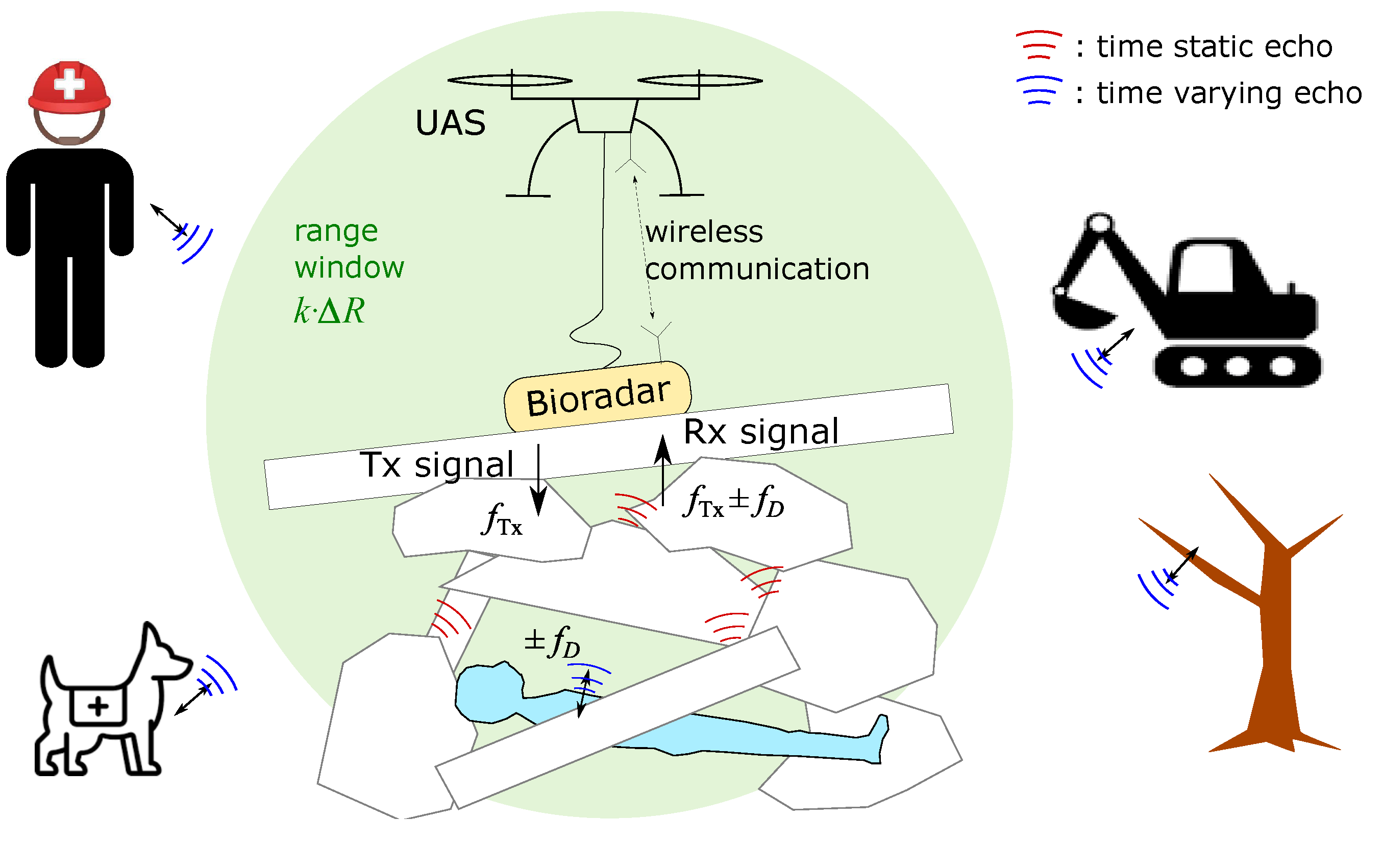
2.1. Bioradar Measuring Principle
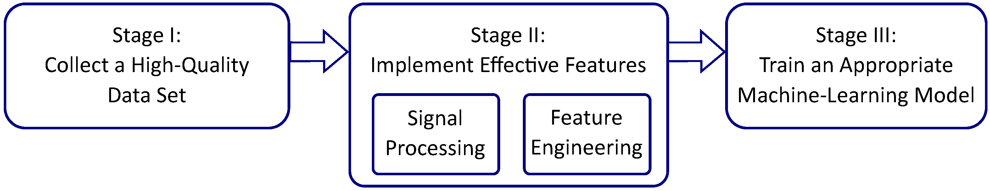
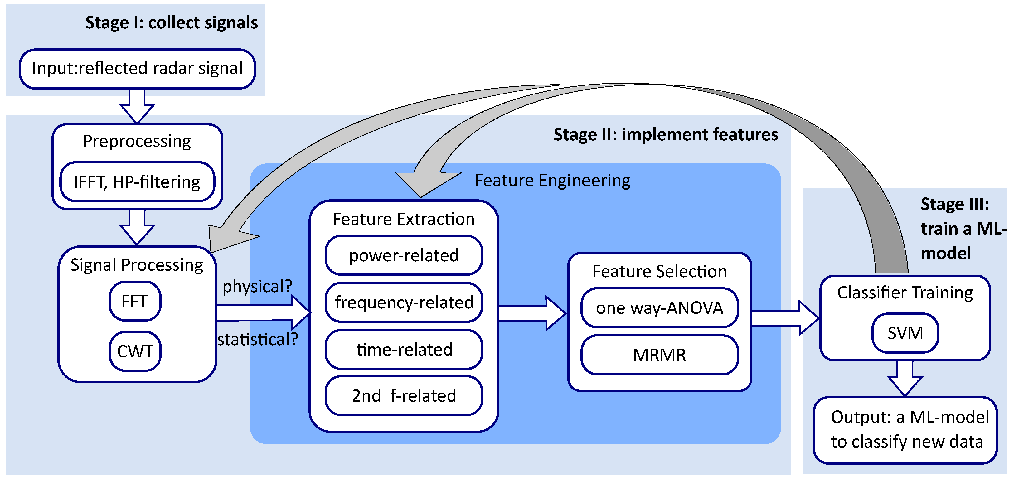
2.2. Workflow and Outline of this Contribution
3. Data Collection
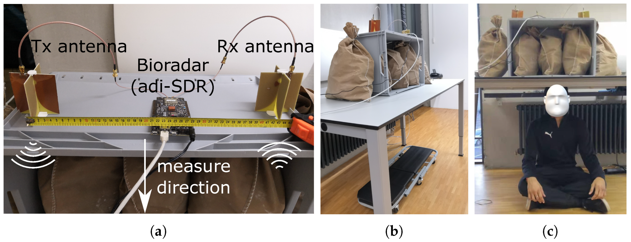
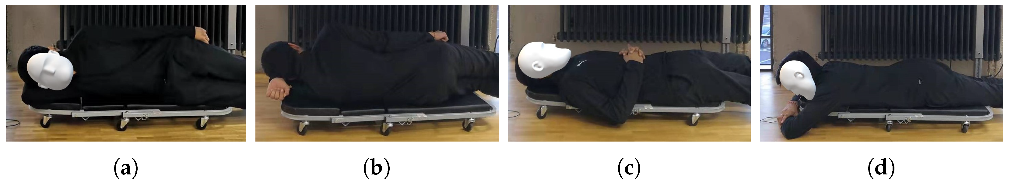
3.1. Experiment
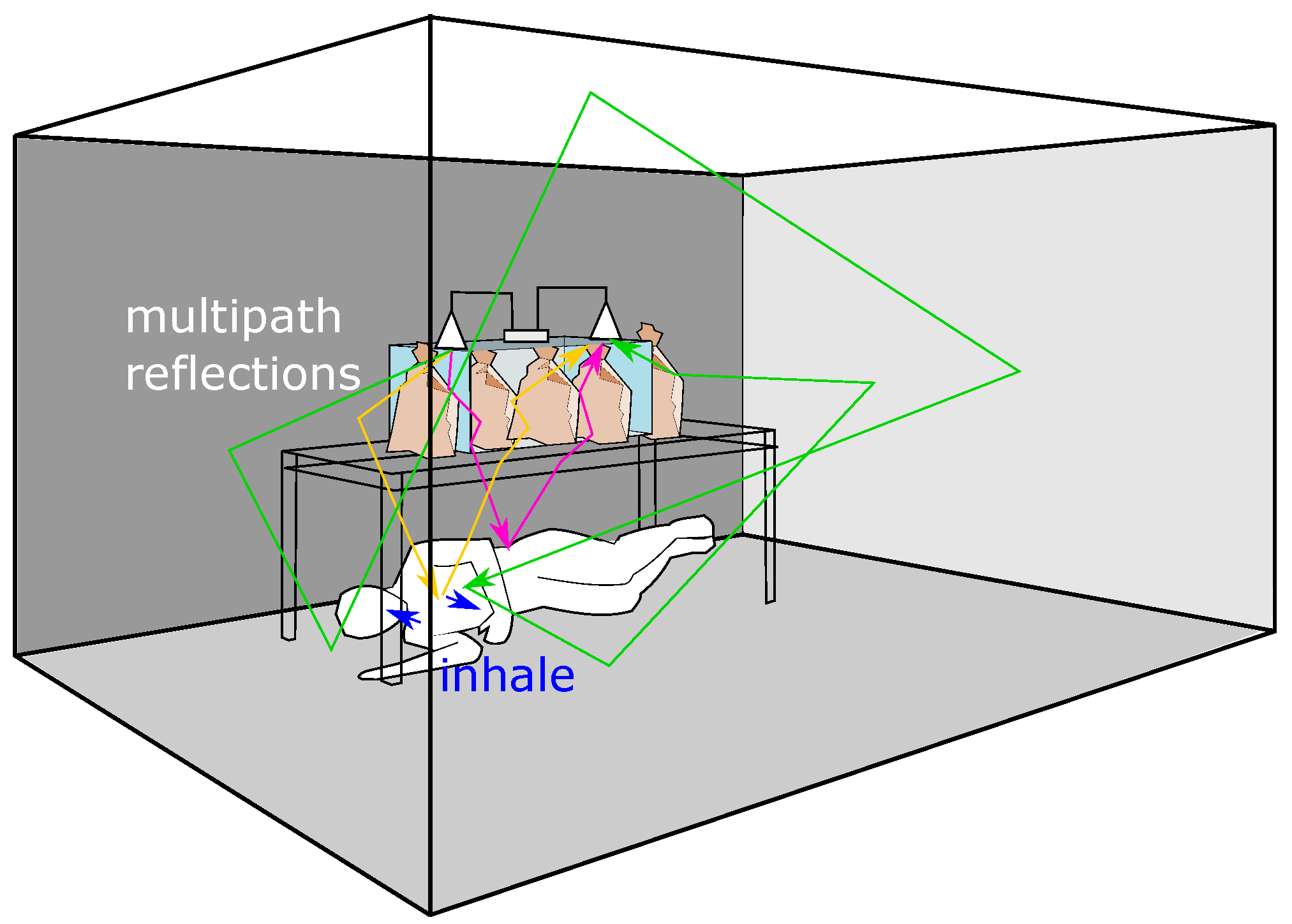
3.2. Obtaining Multiple Virtual Scenes Using Multipath-Reflections
4. Feature Extraction
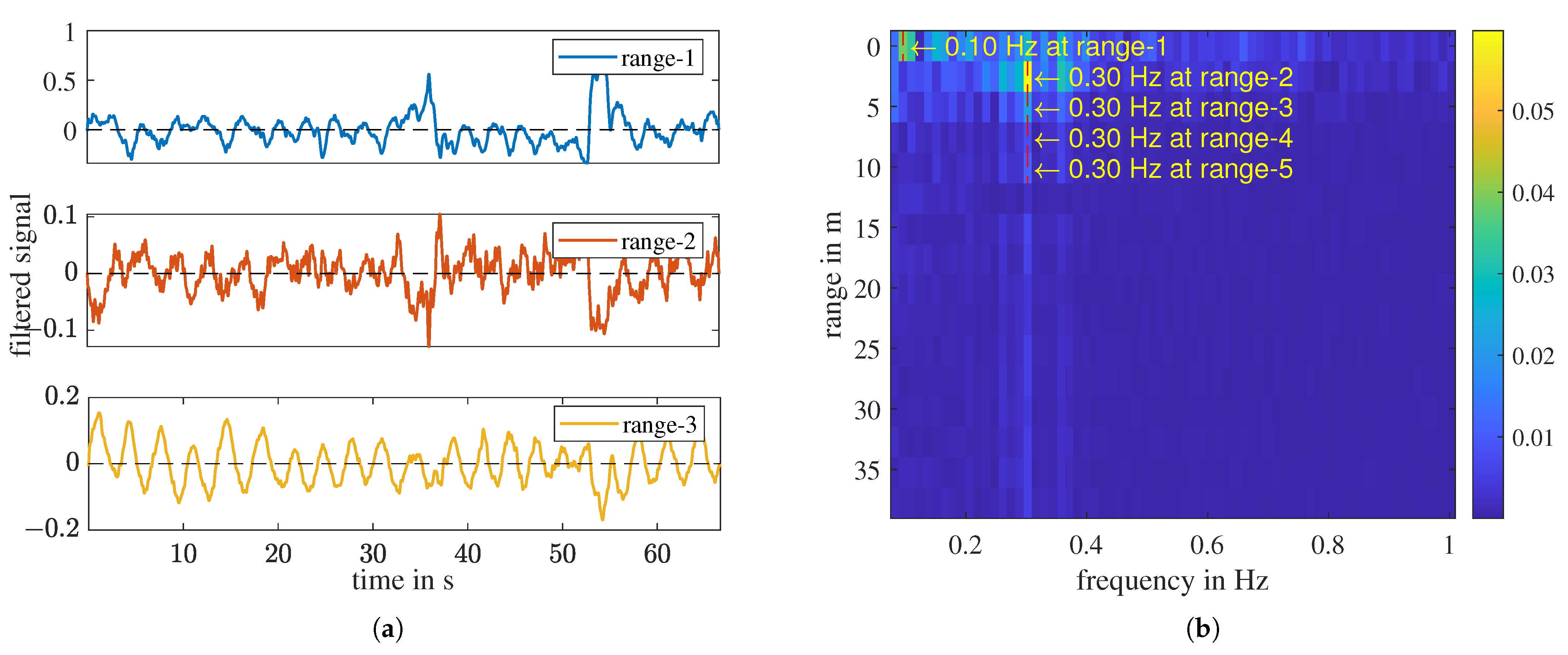
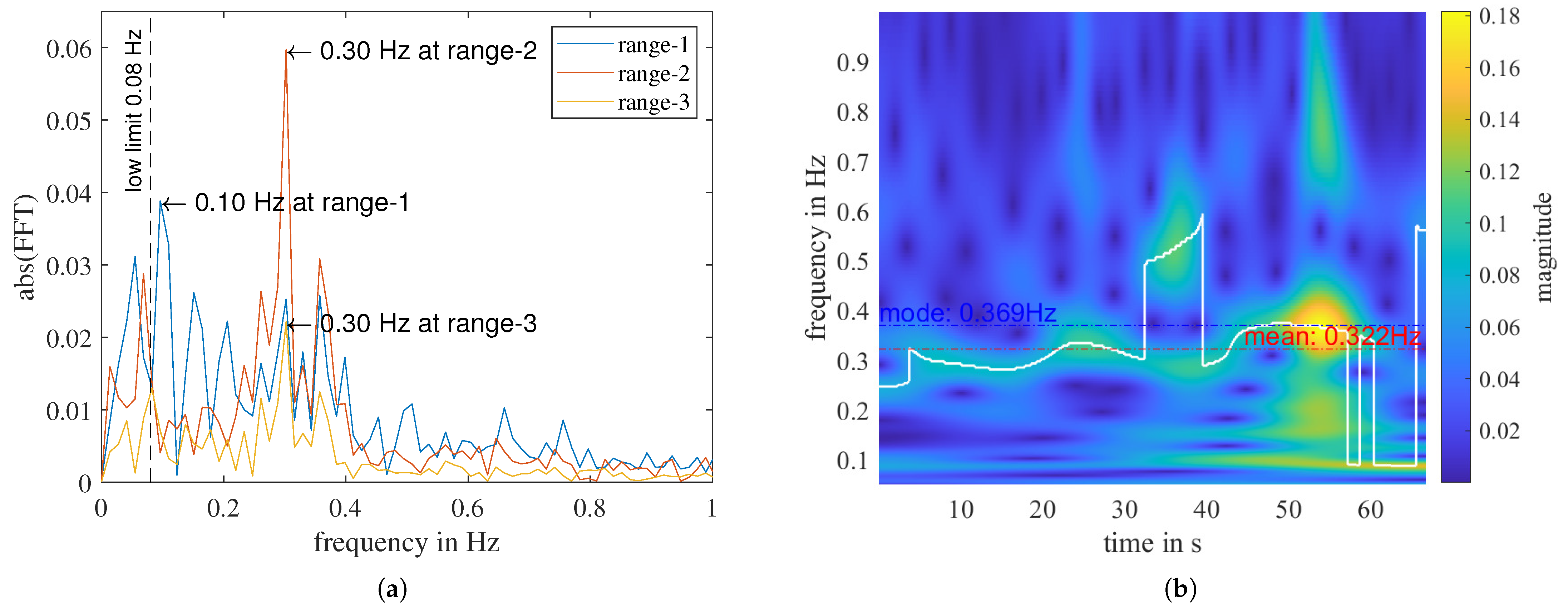
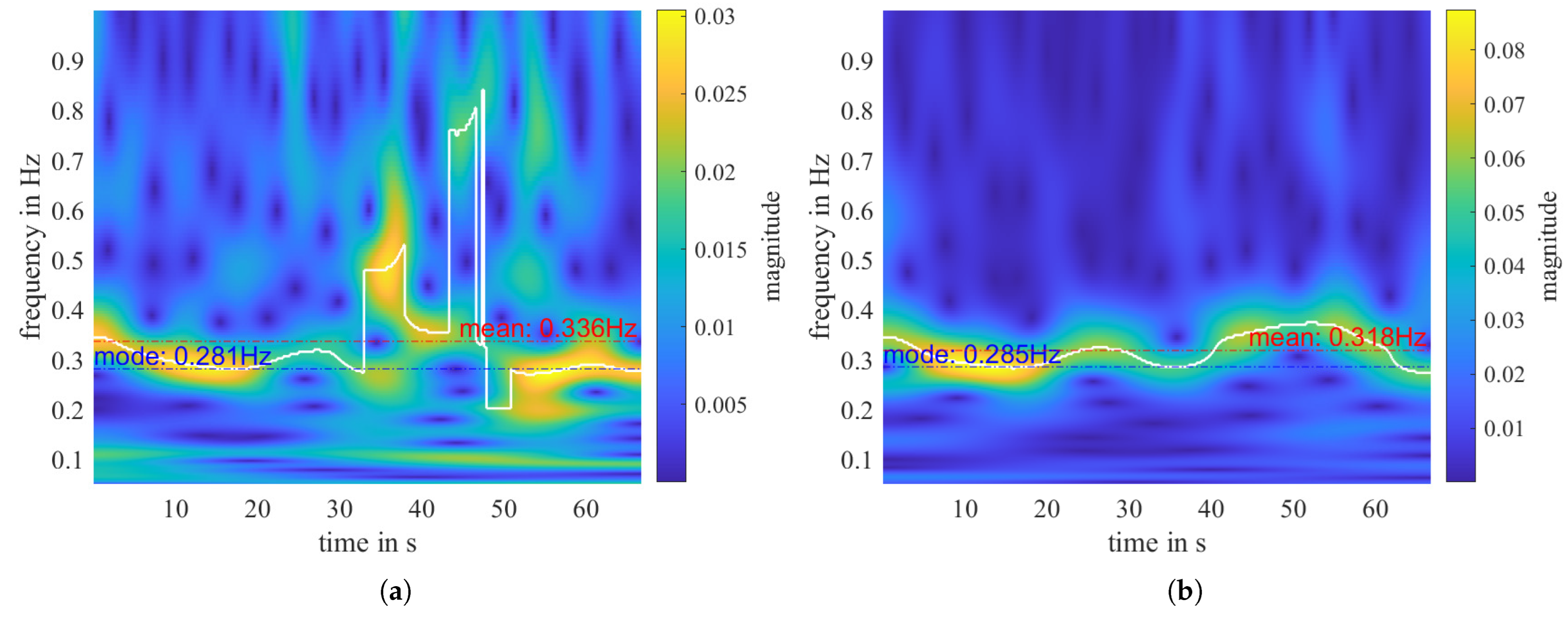
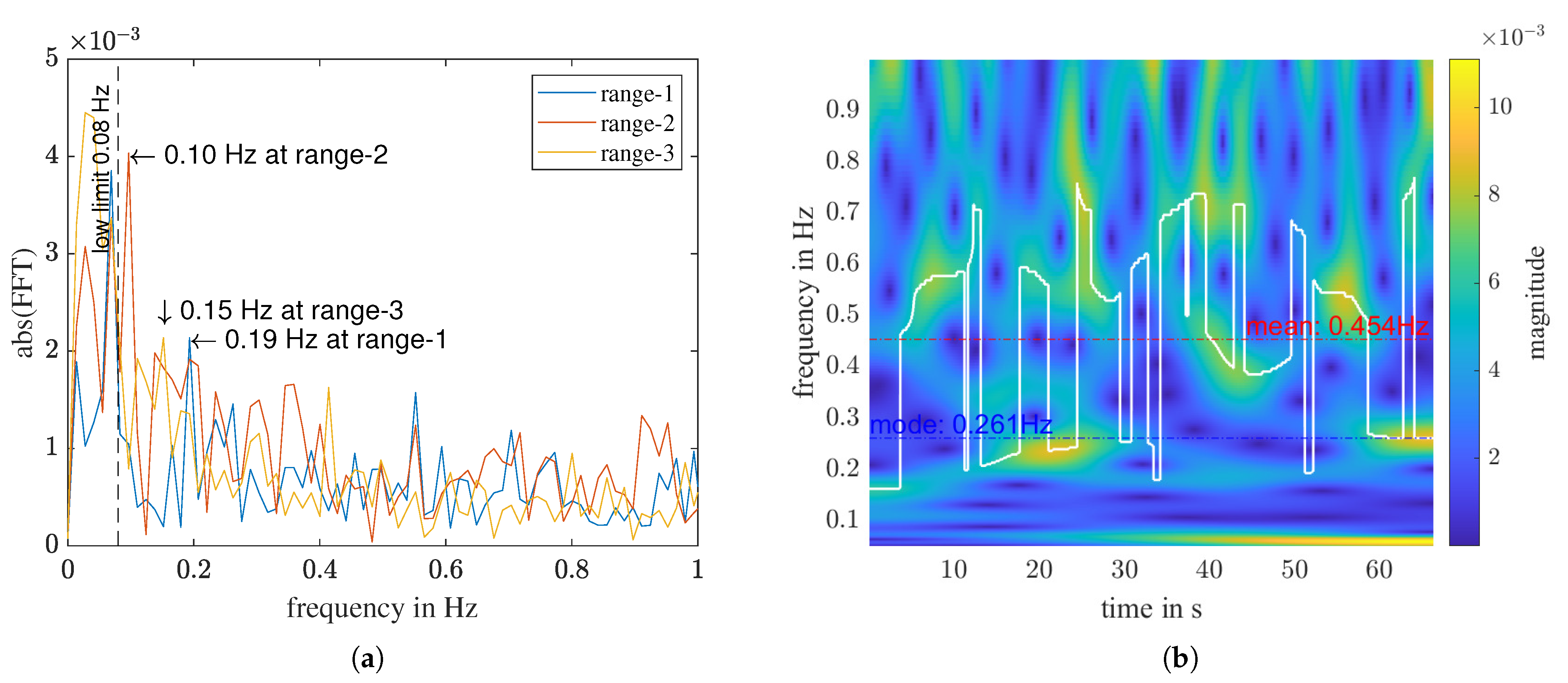
4.1. Physical Features Related to Respiratory Rate
4.2. Statistical Features
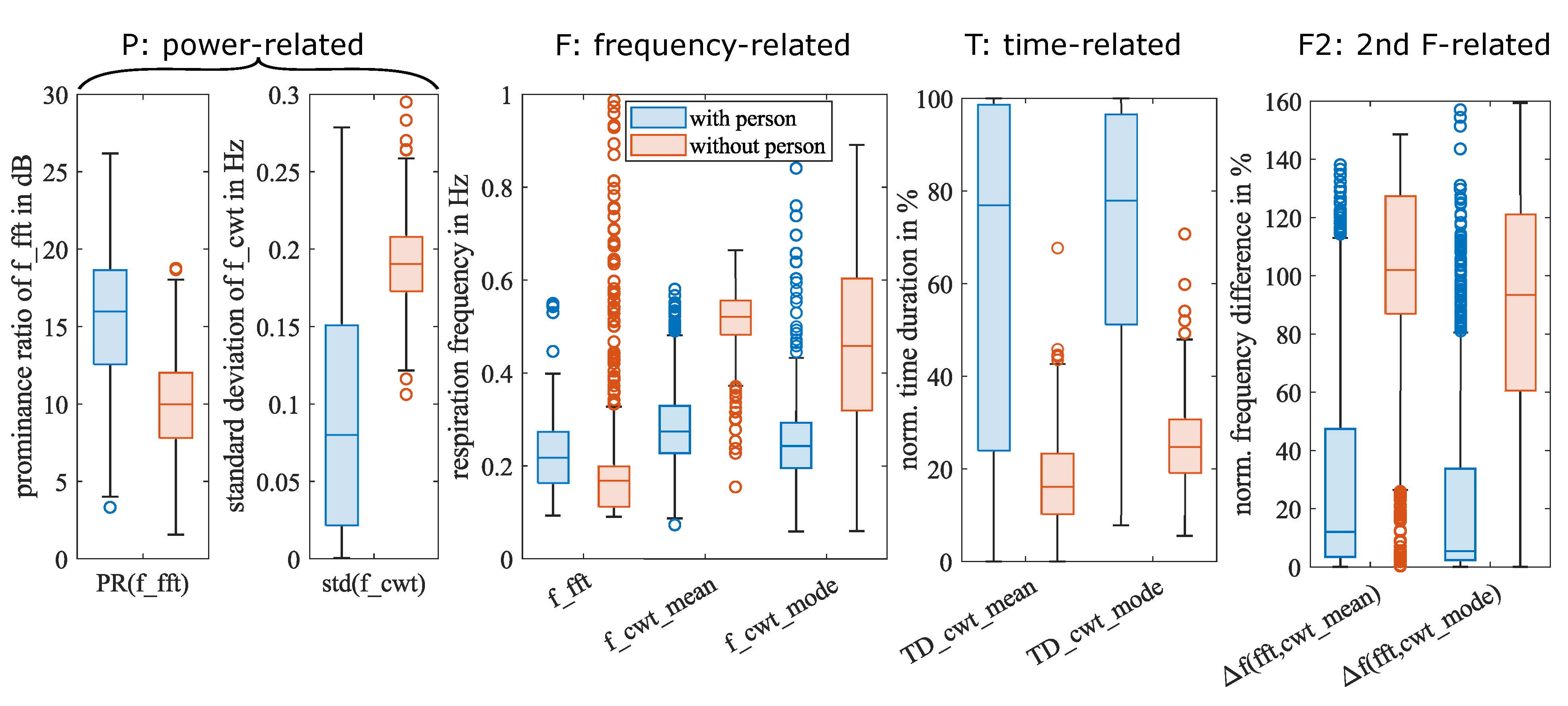
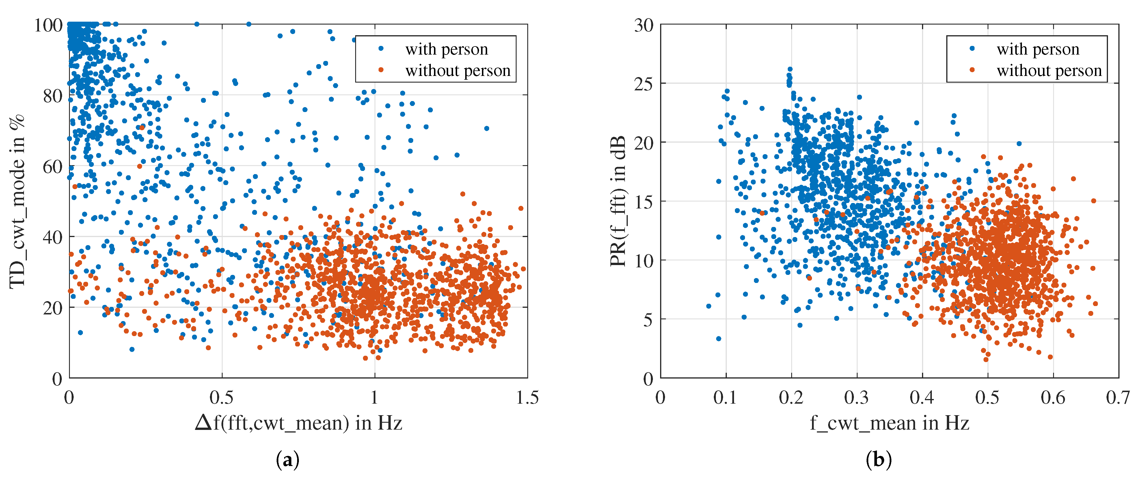
4.3. Summary and Analysis of Extracted Features
5. Feature Selection
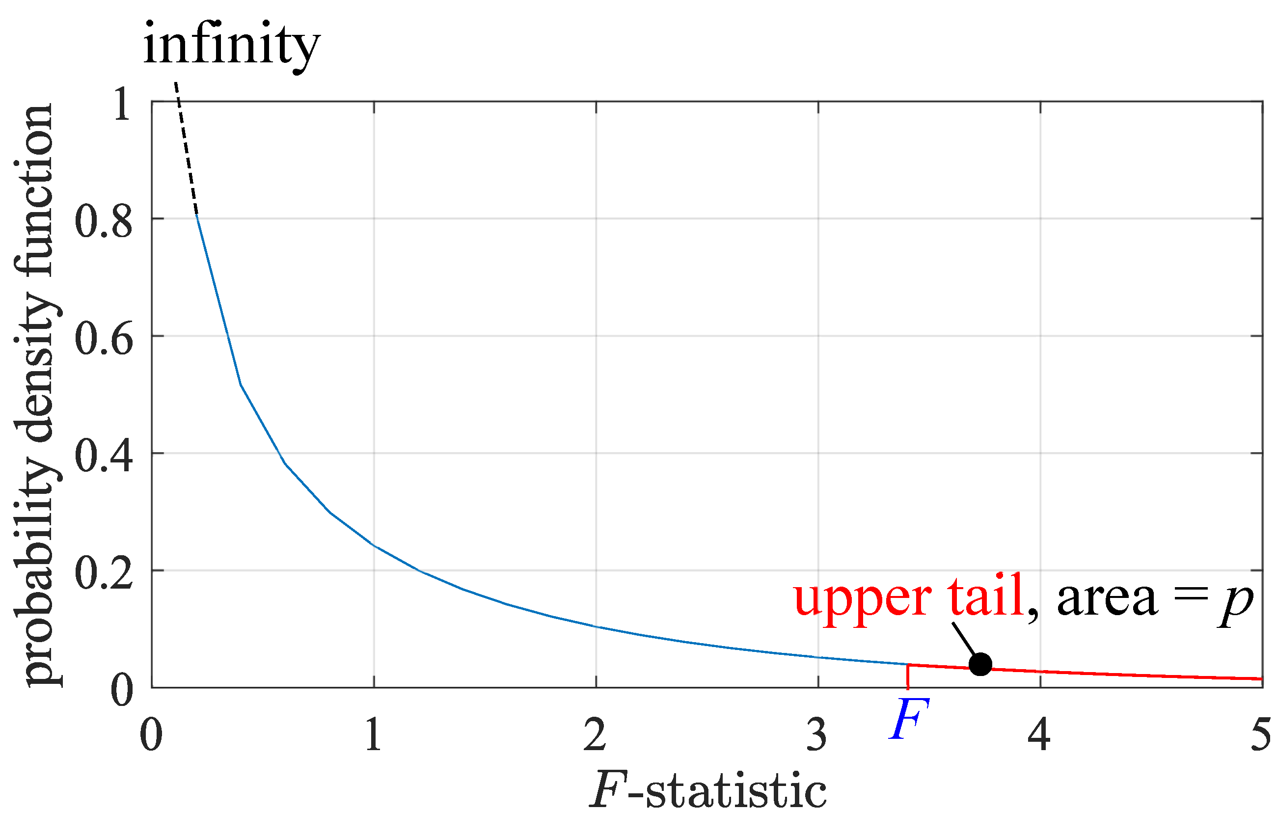
5.1. Basics of One-Way ANOVA
5.2. Basics of MRMR
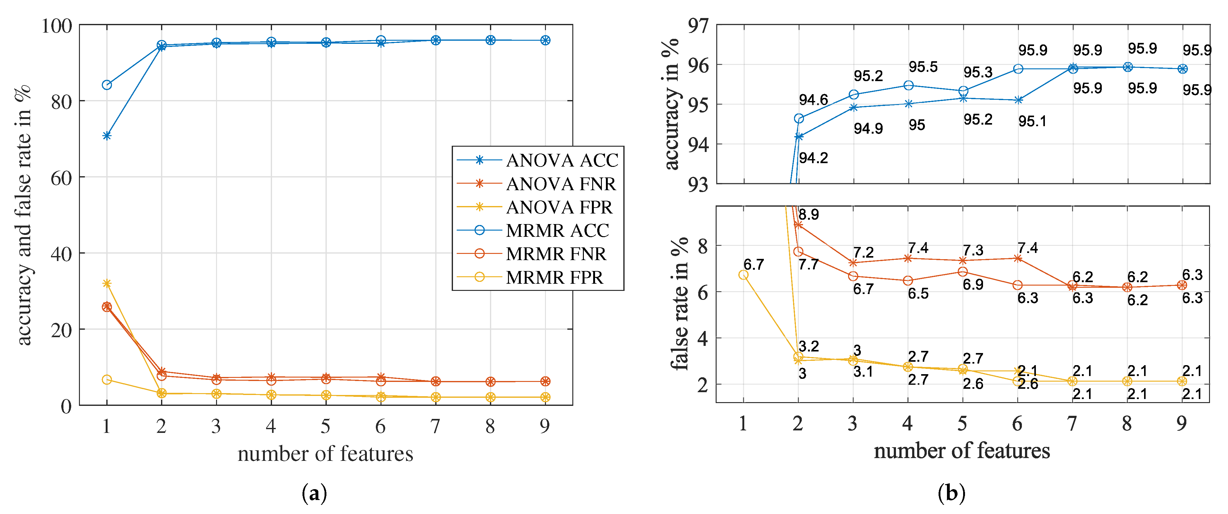
5.3. Ranking Results of Feature Importance
5.4. Investigate the Classification Accuracy of the Trained Models
6. Results and Discussions
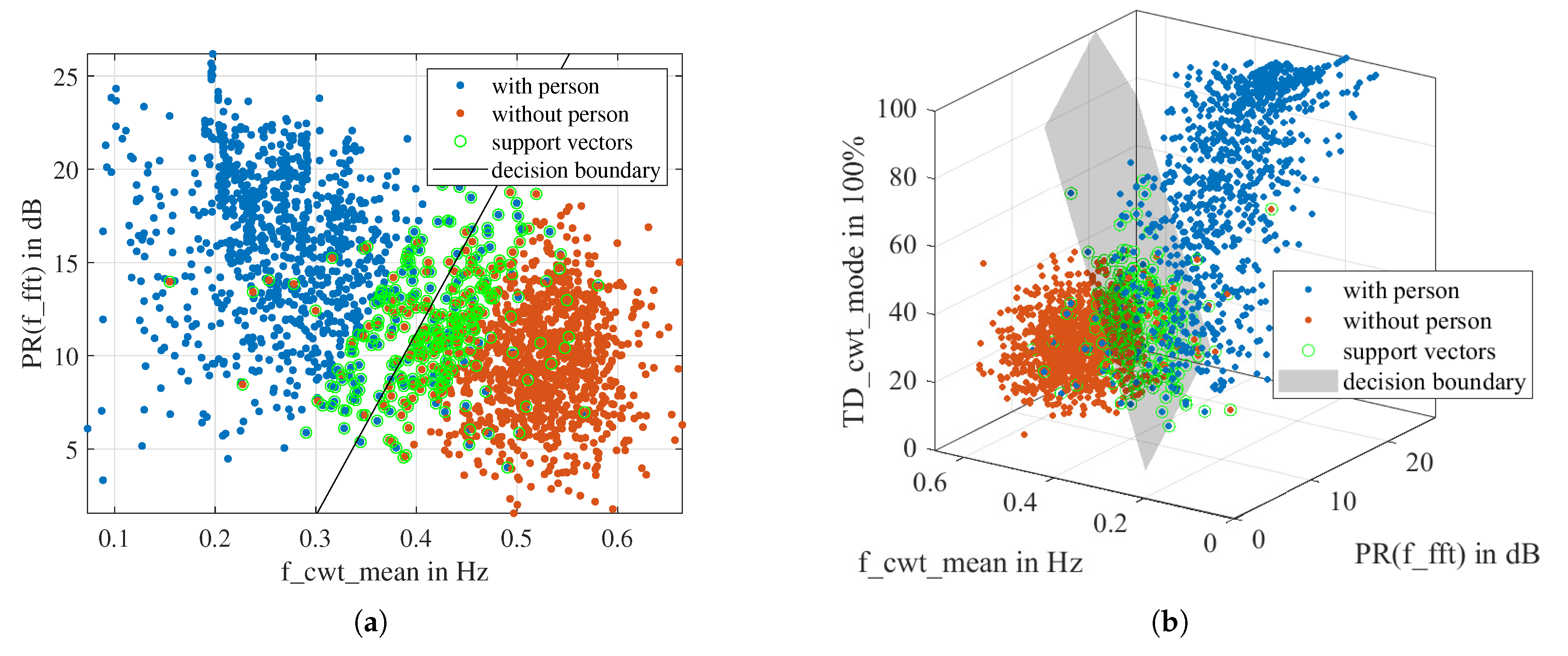
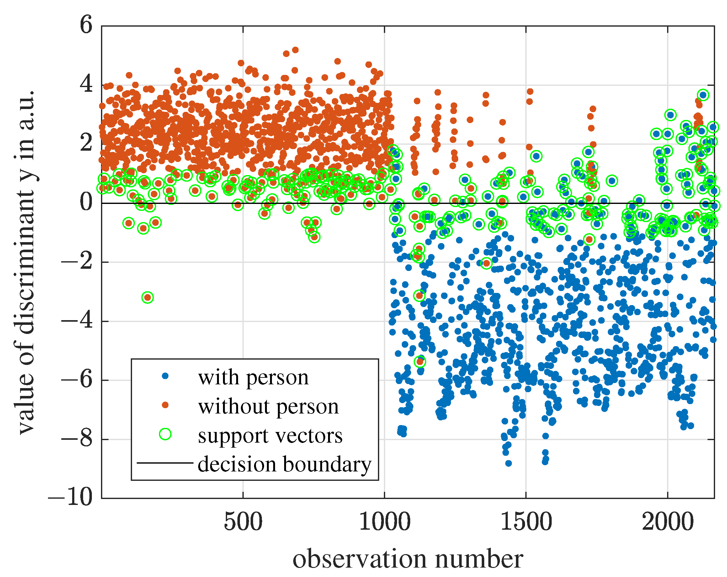
6.1. Hyperplane of Solved SVM Model
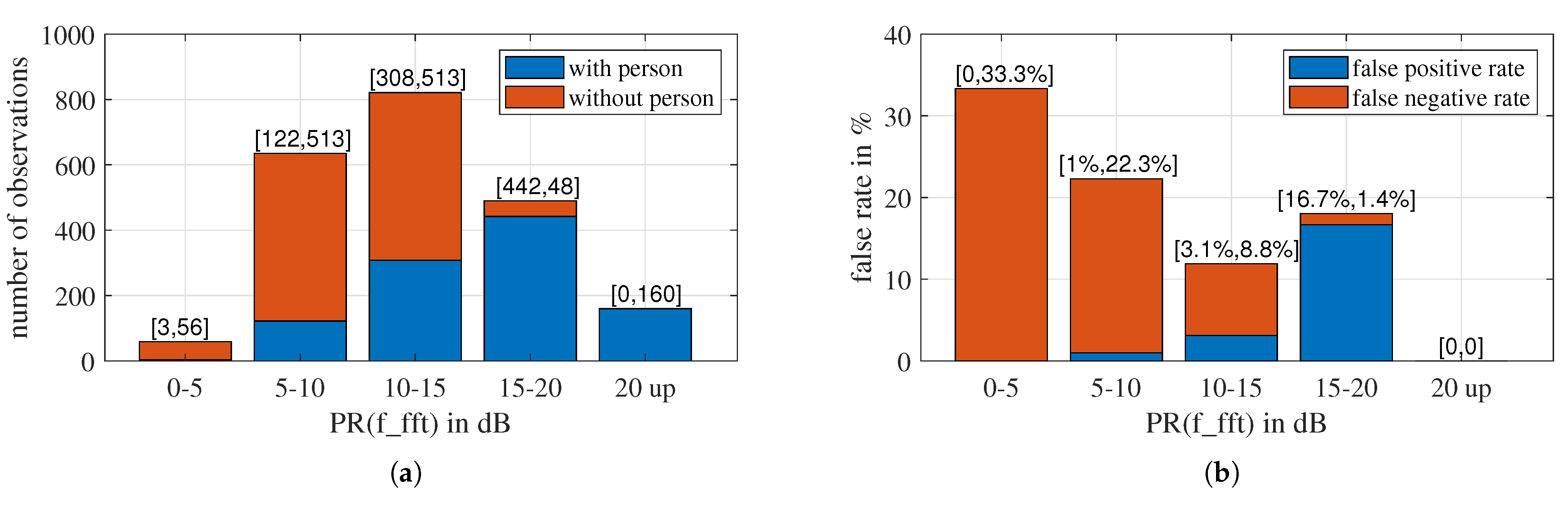
6.2. Impact of Prominence Ratio on False Rate
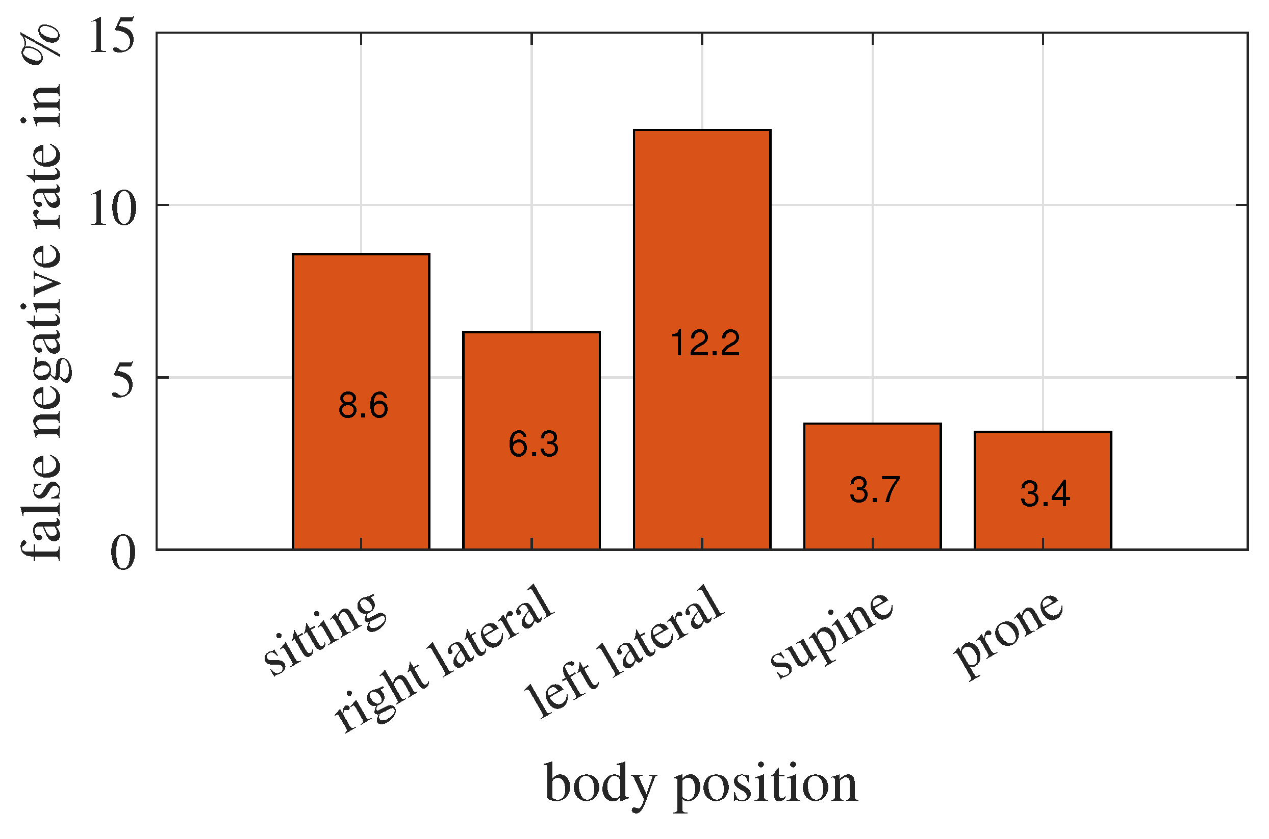
6.3. Effect of Body Position on Breathing Detection in This Particular Experiment
7. Conclusions
Author Contributions
Funding
Institutional Review Board Statement
Informed Consent Statement
Data Availability Statement
Acknowledgments
Conflicts of Interest
References
- SIFO. FOUNT²: Fliegendes Lokalisierungssystem für die Rettung und Bergung von Verschütteten. Available online: https://www.sifo.de/sifo/de/projekte/schutz-und-rettung-von-menschen/innovative-rettungs-und-sicherheitssysteme/fount2/fount2_node.html (accessed on 10 March 2023).
- SIFO. SORTIE: Sensor-Systeme zur Lokalisierung von Verschütteten Personen in Eingestürzten Gebäuden. Available online: https://www.sifo.de/sifo/de/projekte/schutz-und-rettung-von-menschen/internationales-katastrophen-und-risikomanagement/sortie-sensor-systeme-zur-loka-en-in-eingestuerzten-gebaeuden/sortie-sensor-systeme-zur-loka-en-in-eingestuerzten-gebaeuden.html (accessed on 10 March 2023).
- Shi, D.; Aftab, T.; Gidion, G.; Sayed, F.; Reindl, L.M. A novel electrically small ground-penetrating radar patch antenna with a parasitic ring for respiration detection. Sensors 2021, 21, 1930. [Google Scholar] [CrossRef] [PubMed]
- Li, C.; Lubecke, V.M.; Boric-Lubecke, O.; Lin, J. Sensing of life activities at the human-microwave frontier. IEEE J. Microwaves 2021, 1, 66–78. [Google Scholar] [CrossRef]
- Will, C.; Shi, K.; Schellenberger, S.; Steigleder, T.; Michler, F.; Weigel, R.; Ostgathe, C.; Koelpin, A. Local pulse wave detection using continuous wave radar systems. IEEE J. Electromagn. Microwaves Med. Biol. 2017, 1, 81–89. [Google Scholar] [CrossRef]
- Sachs, J.; Helbig, M.; Herrmann, R.; Kmec, M.; Schilling, K.; Zaikov, E. Remote vital sign detection for rescue, security, and medical care by ultra-wideband pseudo-noise radar. Ad Hoc Netw. 2014, 13, 42–53. [Google Scholar] [CrossRef]
- Liu, L.; Liu, S. Remote detection of human vital sign with stepped-frequency continuous wave radar. IEEE J. Sel. Top. Appl. Earth Obs. Remote Sens. 2014, 7, 775–782. [Google Scholar] [CrossRef]
- Shi, D.; Gidion, G.; Aftab, T.; Reindl, L.M.; Rupitsch, S.J. Frequency Comb-Based Ground-Penetrating Bioradar: System Implementation and Signal Processing. Sensors 2023, 23, 1335. [Google Scholar] [CrossRef] [PubMed]
- Hastie, T.; Friedman, J.; Tibshirani, R. The Elements of Statistical Learning; Springer Series in Statistics; Springer: New York, NY, USA, 2001; Volume 27, pp. 83–85. [Google Scholar] [CrossRef]
- Kuhn, M.; Johnson, K. Feature Engineering and Selection: A Practical Approach for Predictive Models; Chapman and Hall/CRC: New York, NY, USA, 2019. [Google Scholar] [CrossRef]
- Zheng, A.; Casari, A. Feature Engineering for Machine Learning: Principles and Techniques for Data Scientists, 1st ed.; O’Reilly Media, Inc.: Sebastopol, CA, USA, 2018. [Google Scholar]
- Dreyfus, G.; Guyon, I. Assessment methods. In Feature Extraction; Springer: Berlin/Heidelberg, Germany, 2006; pp. 65–88. [Google Scholar] [CrossRef]
- Miao, D.; Zhao, H.; Hong, H.; Zhu, X.; Li, C. Doppler radar-based human breathing patterns classification using Support Vector Machine. In Proceedings of the 2017 IEEE Radar Conference (RadarConf), Seattle, WA, USA, 8–12 May 2017; pp. 0456–0459. [Google Scholar] [CrossRef]
- Ma, Y.; Liang, F.; Wang, P.; Lv, H.; Yu, X.; Zhang, Y.; Wang, J. An accurate method to distinguish between stationary human and dog targets under through-wall condition using UWB Radar. Remote Sens. 2019, 11, 2571. [Google Scholar] [CrossRef]
- Zhang, L.; Fu, C.H.; Hong, H.; Xue, B.; Gu, X.; Zhu, X.; Li, C. Non-contact dual-modality emotion recognition system by CW radar and RGB camera. IEEE Sens. J. 2021, 21, 23198–23212. [Google Scholar] [CrossRef]
- Lin, F.; Song, C.; Zhuang, Y.; Xu, W.; Li, C.; Ren, K. Cardiac scan: A non-contact and continuous heart-based user authentication system. In Proceedings of the Annual International Conference on Mobile Computing and Networking, MOBICOM, Snowbird, UT, USA, 16–20 October 2017; Part F1312. pp. 315–328. [Google Scholar] [CrossRef]
- Rahman, A.; Lubecke, V.M.; Boric-Lubecke, O.; Prins, J.H.; Sakamoto, T. Doppler radar techniques for accurate respiration characterization and subject identification. IEEE J. Emerg. Sel. Top. Circuits Syst. 2018, 8, 350–359. [Google Scholar] [CrossRef]
- Skolnik, M.l. Introduction to Radar Systems, 3rd ed.; McGraw-Hill Higher Education: New York, NY, USA, 2001. [Google Scholar]
- Übeyl, E.D.; Güler, I. MATLAB toolboxes: Teaching feature extraction from time-varying biomedical signals. Comput. Appl. Eng. Educ. 2006, 14, 321–332. [Google Scholar] [CrossRef]
- Herzog, M.H.; Francis, G.; Clarke, A. Understanding Statistics and Experimental Design; Learning Materials in Biosciences; Springer: Cham, Switzerland, 2019. [Google Scholar] [CrossRef]
- Ding, C.; Peng, H. Minimum redundancy feature selection from microarray gene expression data. J. Bioinform. Comput. Biol. 2005, 3, 185–205. [Google Scholar] [CrossRef] [PubMed]
- Aly, M. Survey on multiclass classification methods. Neural Netw. 2005, 19, 1–9. [Google Scholar]
- Burges, C.J. A tutorial on support vector machines for pattern recognition. Data Min. Knowl. Discov. 1998, 2, 121–167. [Google Scholar] [CrossRef]
- Steven, W.S. Statistics, Probability and Noise Statistics. In The Scientist & Engineer’s Guide to Digital Signal Processing, 2nd ed.; California Technical Publishing: San Diego, CA, USA, 1999; Chapter 2; pp. 11–34. [Google Scholar]
- Diez, D.; Çetinkaya-Rundel, M.; Barr, C.D. OpenIntro Statistics, 4th ed.; OpenIntro: Boston, MA, USA, 2019. [Google Scholar]
- Darbellay, G.A.; Vajda, I. Estimation of the information by an adaptive partitioning of the observation space. IEEE Trans. Inf. Theory 1999, 45, 1315–1321. [Google Scholar] [CrossRef]
- Zhou, Z.H. Machine Learning; Springer: Singapore, 2021; pp. 181–182. [Google Scholar] [CrossRef]


| # | Feature Notation | Type | Meaning | With Person | Without Person | ||
|---|---|---|---|---|---|---|---|
| 1 | PR(f_fft) | phy. FD-P | prominence ratio in dB | 15.52 dB | 4.26 dB | 9.89 dB | 2.96 dB |
| 2 | std(f_cwt) | stat. TFD-P | standard deviation of f_cwt | 0.09 Hz | 0.07 Hz | 0.19 Hz | 0.03 Hz |
| 3 | f_fft | phy. FD-F | frequency with max(FFT) | 0.22 Hz | 0.08 Hz | 0.18 Hz | 0.12 Hz |
| 4 | f_cwt_mean | stat. TFD-F | mean value of f_cwt | 0.28 Hz | 0.08 Hz | 0.51 Hz | 0.06 Hz |
| 5 | f_cwt_mode | phy. TFD-F | mode value of f_cwt | 0.24 Hz | 0.10 Hz | 0.46 Hz | 0.19 Hz |
| 6 | TD_cwt_mean | stat. TFD-T | norm. duration of f_cwt_mean | 62.9% | 37.1% | 17.2% | 9.4% |
| 7 | TD_cwt_mode | phy. TFD-T | norm. duration of f_cwt_mode | 71.2% | 26.8% | 25.2% | 8.7% |
| 8 | f(fft, cwt_mean) | stat. F2 | norm. diff. btw. f_fft and f_cwt_mean | 29.8% | 35.2% | 101.7% | 30.2% |
| 9 | f(fft, cwt_mode) | stat. F2 | norm. diff. btw. f_fft and f_cwt_mode | 23.9% | 34.1% | 88.2% | 41.7% |
| Ranking | One-Way ANOVA | MRMR | ||
|---|---|---|---|---|
| Feature | Score | Feature | Score | |
| 1 | f(fft, cwt_mean) | Inf. | f_cwt_mean | 0.51 |
| 2 | TD_cwt_mode | Inf. | PR(f_fft) | 0.42 |
| 3 | f_cwt_mean | Inf. | TD_cwt_mode | 0.36 |
| 4 | std(f_cwt) | 687.98 | f(fft, cwt_mode) | 0.34 |
| 5 | TD_cwt_mean | 604.74 | std(f_cwt) | 0.32 |
| 6 | f(fft, cwt_mode) | 580.65 | f(fft, cwt_mean) | 0.29 |
| 7 | PR(f_fft) | 510.40 | f_cwt_mode | 0.28 |
| 8 | f_cwt_mode | 467.40 | TD_cwt_mean | 0.24 |
| 9 | f_fft | 33.26 | f_fft | 0.12 |
| 2D-LSVM | 3D-LSVM | 4D-LSVM | ||||||
|---|---|---|---|---|---|---|---|---|
| s | b | s | b | s | b | |||
| 0.11 | −0.17 | 0.25 | −0.62 | 0.43 | −0.69 | |||
| feature | ||||||||
| PR(f_fft) | 12.58 | 4.60 | −0.09 | −0.19 | −0.31 | |||
| f_cwt_mean | 0.40 | 0.14 | 0.25 | 0.50 | 0.79 | |||
| TD_cwt_mode | 0.47 | 0.30 | / | −0.26 | −0.41 | |||
| f(fft, cwt_mean) | 0.67 | 0.49 | / | / | 0.18 | |||
| accuracy | / | 94.6% | 95.2% | 95.7% | ||||
| PR(f_fft) | f_cwt_mean | TD_cwt_mode | f(fft, cwt_mean) | Prediction | ||
|---|---|---|---|---|---|---|
| range-1 | 13.39 | 0.32 | 0.37 | 1.08 | −1.25 | with person |
| range-2 | 17.83 | 0.34 | 0.70 | 0.11 | −3.62 | with person |
| range-3 | 16.28 | 0.32 | 0.69 | 0.05 | −3.66 | with person |
| range-4 | 14.54 | 0.32 | 0.74 | 0.05 | −3.55 | with person |
| range-5 | 17.25 | 0.40 | 0.13 | 0.28 | −0.72 | with person |
| PR(f_fft) | f_cwt_mean | TD_cwt_mode | f(fft, cwt_mean) | Prediction | ||
|---|---|---|---|---|---|---|
| range-1 | 10.20 | 0.45 | 0.23 | 0.81 | 1.24 | without person |
| range-2 | 11.59 | 0.35 | 0.35 | 1.14 | −0.46 | with person |
| range-3 | 10.67 | 0.44 | 0.25 | 0.97 | 1.04 | without person |
| range-4 | 11.35 | 0.55 | 0.26 | 0.81 | 2.27 | without person |
| range-5 | 11.12 | 0.53 | 0.26 | 1.38 | 2.53 | without person |
Disclaimer/Publisher’s Note: The statements, opinions and data contained in all publications are solely those of the individual author(s) and contributor(s) and not of MDPI and/or the editor(s). MDPI and/or the editor(s) disclaim responsibility for any injury to people or property resulting from any ideas, methods, instructions or products referred to in the content. |
© 2023 by the authors. Licensee MDPI, Basel, Switzerland. This article is an open access article distributed under the terms and conditions of the Creative Commons Attribution (CC BY) license (https://creativecommons.org/licenses/by/4.0/).
Share and Cite
Shi, D.; Gidion, G.; Reindl, L.M.; Rupitsch, S.J. Automatic Life Detection Based on Efficient Features of Ground-Penetrating Rescue Radar Signals. Sensors 2023, 23, 6771. https://doi.org/10.3390/s23156771
Shi D, Gidion G, Reindl LM, Rupitsch SJ. Automatic Life Detection Based on Efficient Features of Ground-Penetrating Rescue Radar Signals. Sensors. 2023; 23(15):6771. https://doi.org/10.3390/s23156771
Chicago/Turabian StyleShi, Di, Gunnar Gidion, Leonhard M. Reindl, and Stefan J. Rupitsch. 2023. "Automatic Life Detection Based on Efficient Features of Ground-Penetrating Rescue Radar Signals" Sensors 23, no. 15: 6771. https://doi.org/10.3390/s23156771
APA StyleShi, D., Gidion, G., Reindl, L. M., & Rupitsch, S. J. (2023). Automatic Life Detection Based on Efficient Features of Ground-Penetrating Rescue Radar Signals. Sensors, 23(15), 6771. https://doi.org/10.3390/s23156771