


Heuristics and Learning Models for Dubins MinMax Traveling Salesman Problem

Abstract
:1. Introduction
Contributions of This Article
- We formulate a mixed-integer linear program for the MD-GmTSP (Section 3).
- We explore learning-based methods to solve the MD-mTSP. An architecture consisting of a shared graph neural network and distributed policy networks is used to define a learning policy for MD-GmTSP. Reinforcement learning is used to learn the allocation of agents to vertices to generate feasible solutions for the MD-GmTSP, thus eliminating the need for accurate ground truth (Section 6).
2. Literature Review
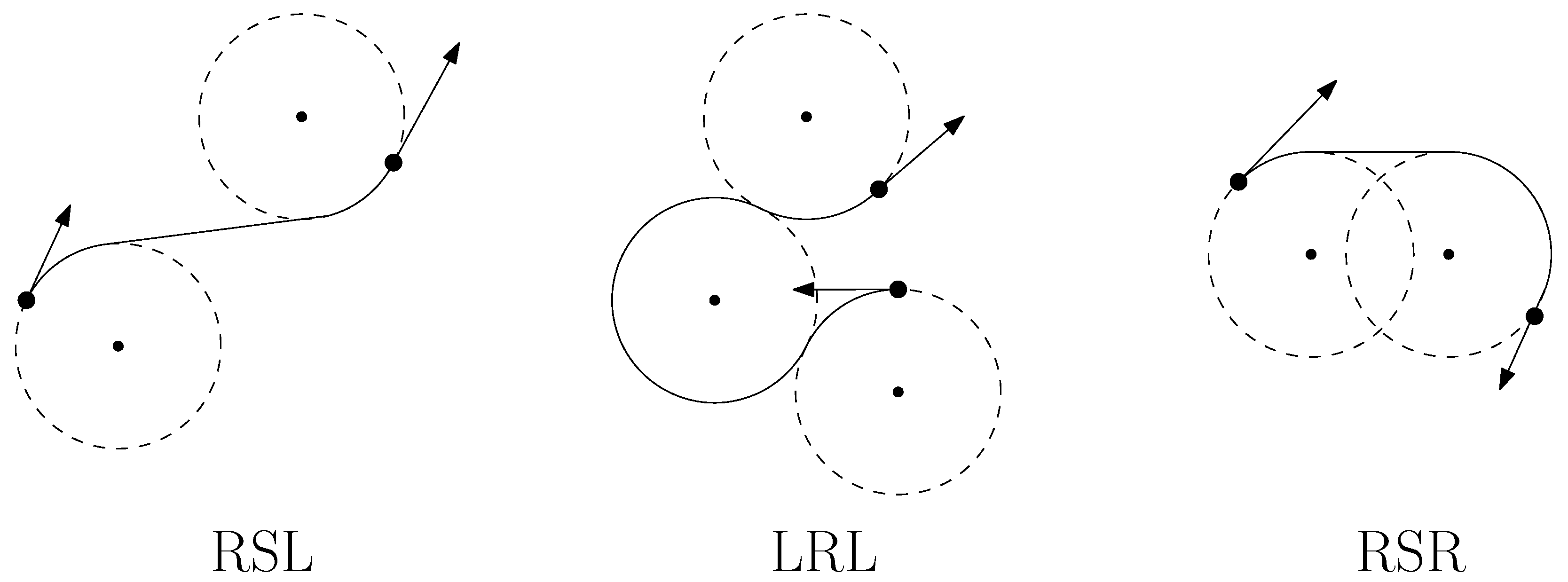
3. Problem Statement
- Each target in T is visited once by some vehicle at a specified heading angle;
- The tour for each vehicle starts and ends at the depot;
- The length of the longest Dubins tour among the m vehicles is minimized.
4. Mixed-Integer Linear Programming Formulation
4.1. Notations
- , the set of all possible Dubins vehicle configurations. Let V be partitioned into mutually exclusive and exhaustive non-empty sub-sets where corresponds to the configuration at the depot, and corresponds to the t target clusters.
- , the set of arcs representing the Dubins path between configurations.
- , the set of homogeneous (uniform) vehicles that serve these customers.
- , the cost of traveling from configuration i to configuration j for vehicle k, where , , , , , .
- , the rank order (visit order) of cluster on the tour of vehicle , .
- , the maximum number of clusters that a vehicle can visit.
4.2. Decision Variables
4.3. Cluster Degree Constraints
4.4. Cluster Connectivity Constraints
4.5. Sub-Tour Elimination Constraints
4.6. Objective
4.7. Solving the MILP
5. Heuristics for the MD-GmTSP
5.1. Initial Solution: Construction Phase
| Algorithm 1 Greedy k-insertion for MD-GmTSP. |
Initialization: Start with m initial Dubins tours starting and ending at the depot . Repeat: While the set of unvisited targets is non-empty
|
| Algorithm 2 Cheapest k-insertion for MD-GmTSP |
Initialization: Start with m initial Dubins tours starting and ending at the depot . Repeat: While the set of unvisited targets is non-empty
|
5.2. Neighborhood Search: Improvement Phase
5.2.1. Basic Variable Neighborhood Search (BVNS)
| Algorithm 3 Steps of the basic VNS by Hansen and Mladenovic [73] |
Initialization: Choose a set of neighborhood structures denoted by for the search process; find an initial solution x; select a termination/stopping condition and repeat the following steps until the termination condition is met:
|
Neighborhood Structures
- (1)
- and differ only in the order of target visits in the tour of vehicle .
- (2)
- The tour for vehicle in differs from the tour of vehicle in by at most k edges.
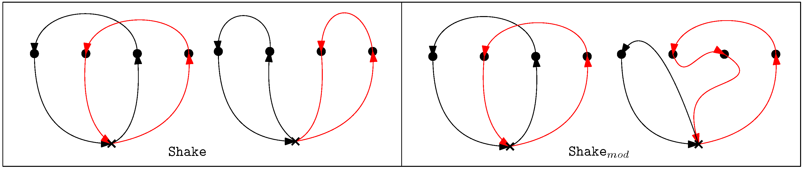
Shake
Local Search
| Algorithm 4 SteepestDescent Heuristic by Hansen and Mladenovic [73] |
Initialization: Find an initial solution x; Choose the neighborhood structures , and the objective function that calculates the length of the longest tour in x, Repeat:
|
| Algorithm 5 FirstImprovement heuristic by Hansen and Mladenovic [73] |
Initialization: Find an initial solution x; Choose the neighborhood structures , and the objective function that calculates the length of the longest tour in x, Repeat:
|
2-opt
3-opt
| Algorithm 6 Steps for neighborhood change by Hansen and Mladenovic [73] |
|
5.2.2. Variable Neighborhood Descent (VND)
| Algorithm 7 Steps of the basic VND by Hansen and Mladenovic [73] |
Initialization: Choose a set of neighborhood structures denoted by that will be used in the descent process; find an initial solution x; select a termination/stopping condition and repeat the following steps until the termination condition is met:
|
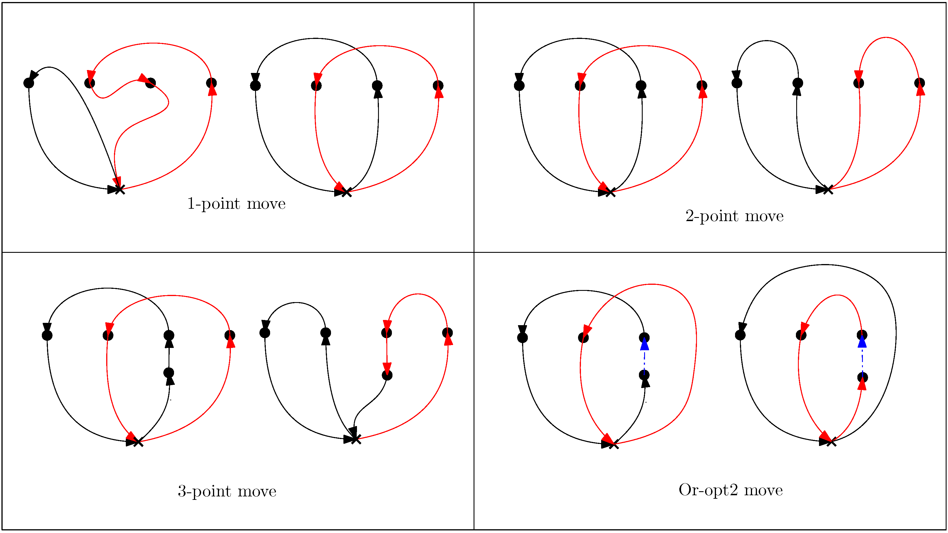
Exploration of Neighborhoods for MD-GmTSP
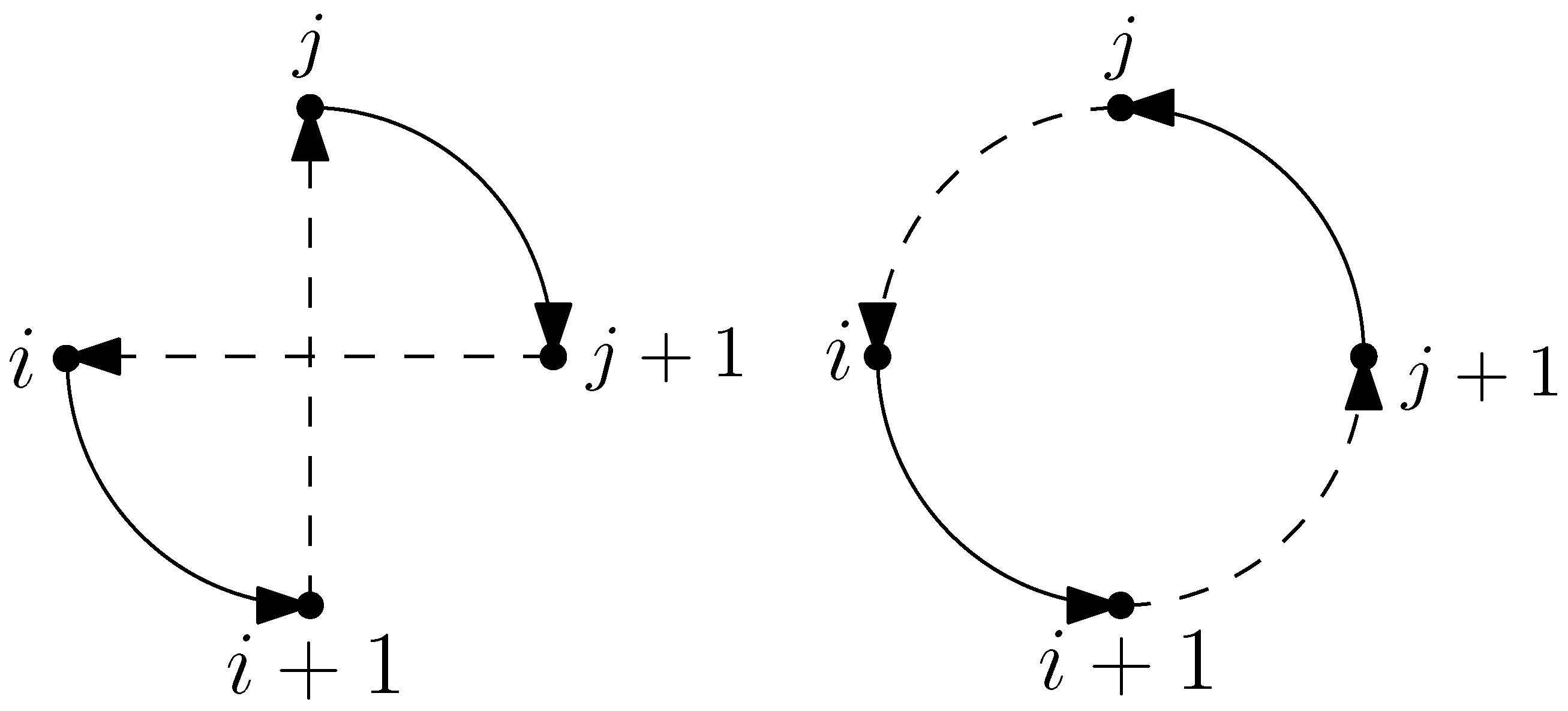
- One-point move: Given a solution x, a one-point move transfers a target from tour to a new feasible position in another tour . The target to be moved is chosen from the tour having the largest tour length and is relocated to a tour having the smallest tour length. The computational complexity of these local search operators is for a given solution .
- Two-point move: A two-point move swaps a pair of nodes rather than transferring a node between tours as in a one-point move. A target belonging to the tour having the largest tour length is swapped with a target belonging to another tour . After performing two-point moves from the solution , the best solution is returned depending on the search strategy employed (FirstImprovement or SteepestDescent).
5.2.3. General Variable Neighborhood Search (GVNS)
| Algorithm 8 Steps of the GVNS by Hansen and Mladenovic [73] |
Initialization: Choose the set of neighborhood structures denoted by that will be used in the shaking phase and the set of neighborhood structures that will be used in the local search process; find an initial solution x; choose a termination/stopping condition. Repeat the following steps until the termination condition is met:
|
Neighborhood Search Structures for MD-GmTSP
- 1.
- One-point move: In GVNS, we use the same One-point move operator as in BVNS.
- 2.
- Two-point move: In GVNS, we use the same Two-point move operator as in BVNS.
- 3.
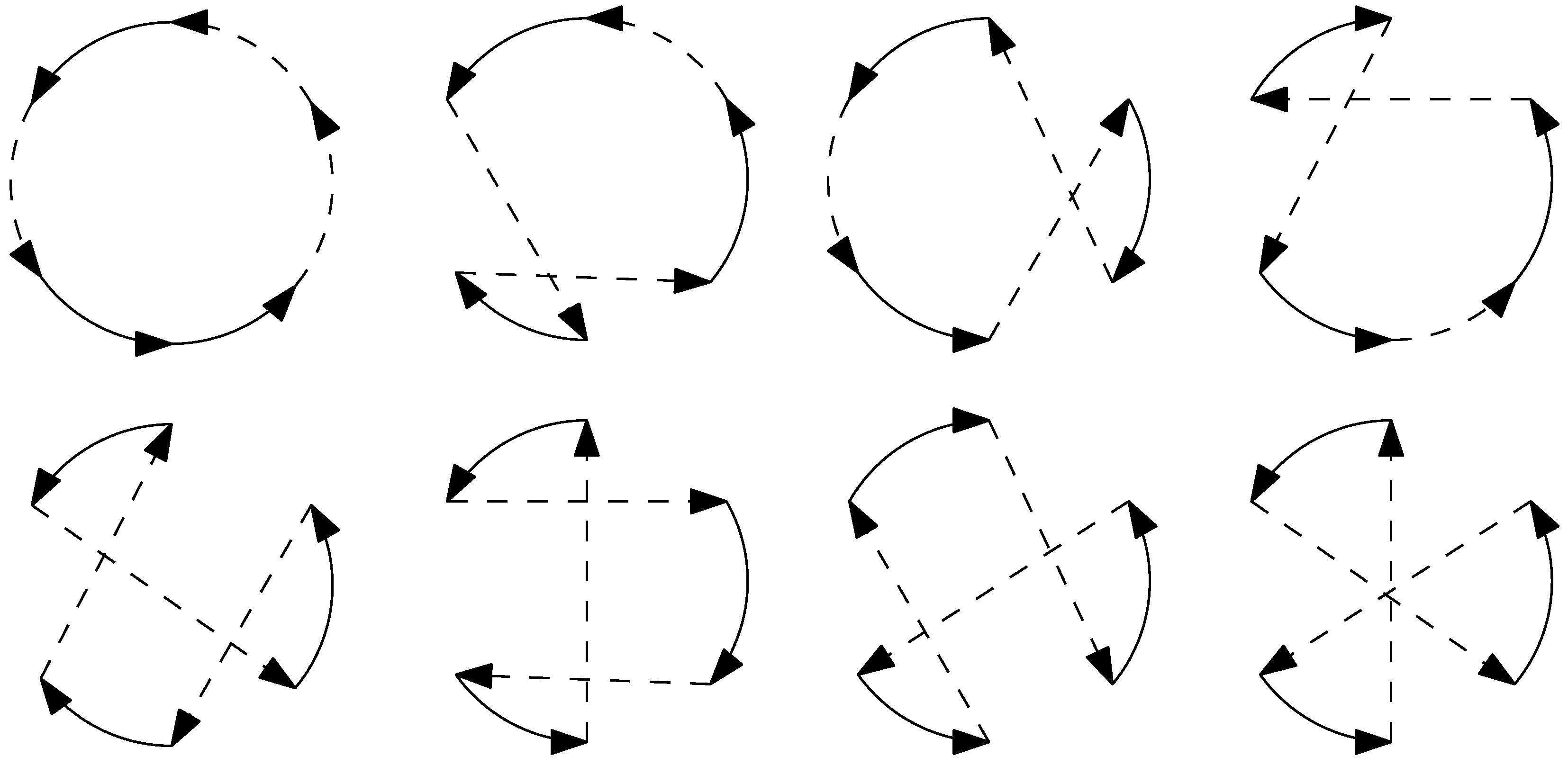
- Or-opt2 move: An or-opt2 move selects a string of two adjacent nodes belonging to the tour having the maximum length and transfers it into a new tour. After performing the or-opt2 move for all strings of nodes , the best solution is returned by the operator depending on the search strategy employed. The or-opt2 operator generates as compared to generic or-optk move operator generates . For our use case, no improvement was observed for , which can be attributed to the complexity in the MD-GmTSP problem.
- 4.
- Three-point move: The three-point move operation involves selecting a pair of adjacent nodes from the tour with the maximum length and exchanging them with a node from another tour. By repeatedly applying three-point moves starting from the initial solution , the operator generates a new solution . Depending on the chosen search strategy, the best solution is returned by the operator.
- 5.
- 2-opt move: We use a 2-opt move operator to improve the resulting tours obtained from the rest of the operators by performing intra-tour local optimization.
Local Search by VND for MD-GmTSP
| Algorithm 9 |
|
6. Learning-Based Approach for the MD-GmTSP
6.1. Framework Architecture
6.1.1. Graph Embedding
6.1.2. Distributed Policy Networks
Calculation of Agent Embedding
- Graph Context embedding: A graph context embedding is used to ensure that every city, except the depot, is visited by only one agent and the depot is visited by all agents. By setting the depot as the first node in the graph (), we concatenate the depot features with the global embedding to create the graph context embedding, represented as . The concatenation operation is denoted by and is shown in Equation (12):
- Attention Mechanism: The attention mechanism [90] is used to convey the importance of a node to an agent a. The node feature set obtains the keys and values, and the graph context embedding computes the query for agent a, which is standard for all agents.where and are the dimension of key and values. A SoftMax is used to compute the attention weights , which the agent puts on node i, using:where is the compatibility of the query to be associated with the agent and all its nodes given by
- Agent embedding: From the attention weights, we construct the agent embedding using
S-Samples Batch Reinforcement Learning
7. Computational Results
7.1. MILP Results
7.2. VNS-Based Heuristics Results
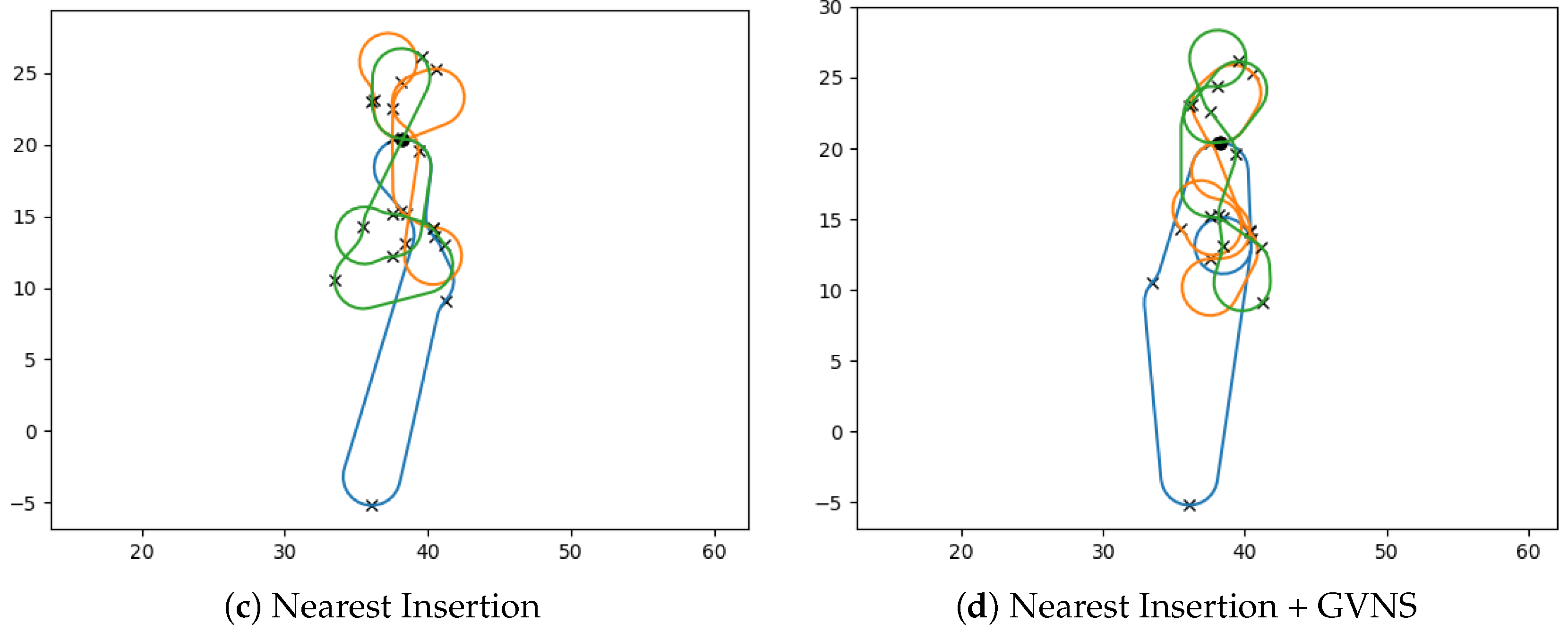
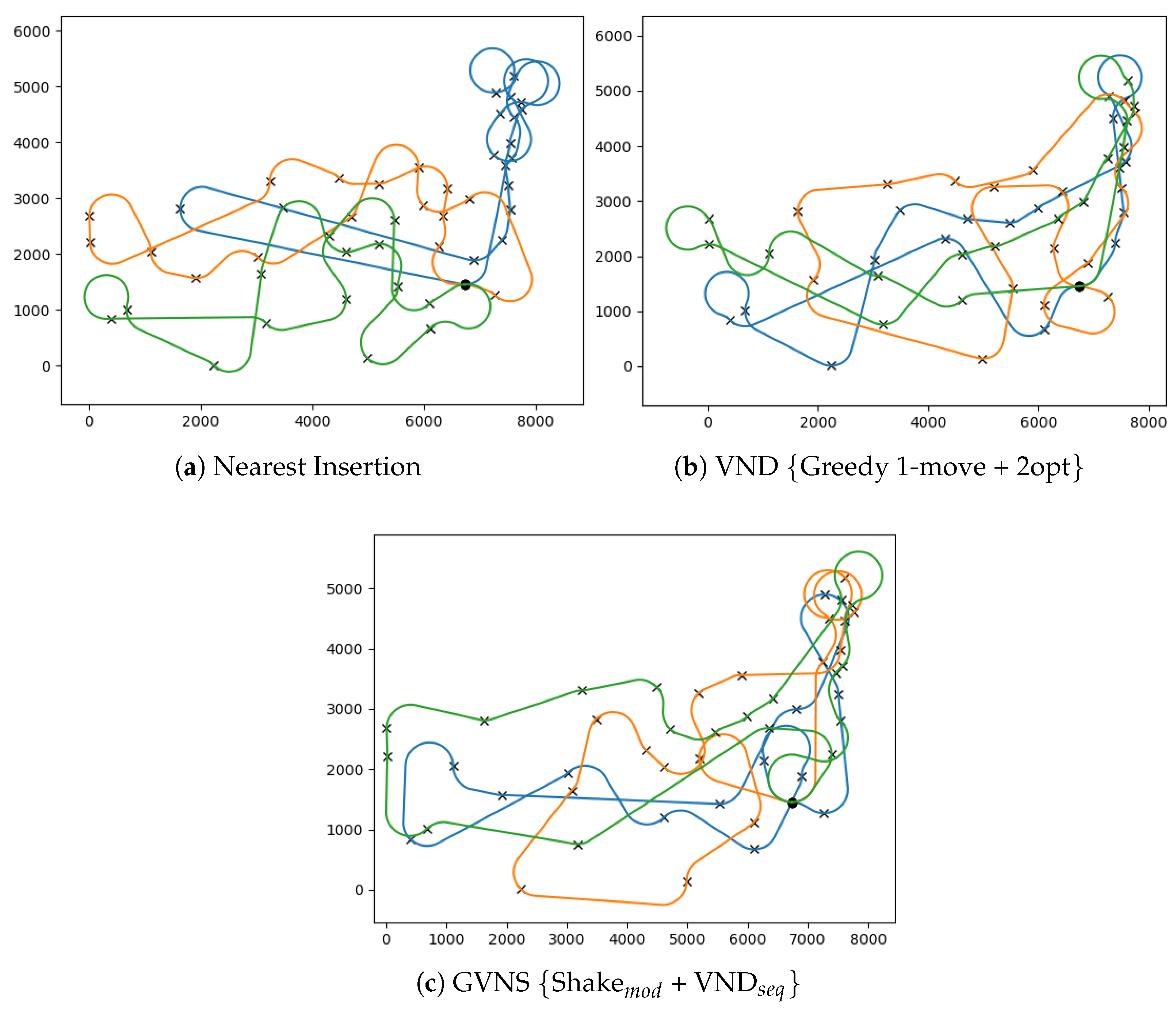
7.2.1. Quality of Initial Feasible Solutions
7.2.2. Analysis of VNS Improvements for MD-GmTSP
7.3. Learning-Based Approach
8. Conclusions
Author Contributions
Funding
Institutional Review Board Statement
Informed Consent Statement
Data Availability Statement
Conflicts of Interest
References
- Lawler, E.L.; Lenstra, J.K.; Rinnooy Kan, A.H.; Shmoys, D.B. Erratum: The traveling salesman problem: A guided tour of combinatorial optimization. J. Oper. Res. Soc. 1986, 37, 655. [Google Scholar] [CrossRef]
- Laporte, G. The traveling salesman problem: An overview of exact and approximate algorithms. Eur. J. Oper. Res. 1992, 59, 231–247. [Google Scholar] [CrossRef]
- Boscariol, P.; Gasparetto, A.; Scalera, L. Path Planning for Special Robotic Operations. In Robot Design: From Theory to Service Applications; Carbone, G., Laribi, M.A., Eds.; Springer International Publishing: Cham, Switzerland, 2023; pp. 69–95. [Google Scholar] [CrossRef]
- Ham, A.M. Integrated scheduling of m-truck, m-drone, and m-depot constrained by time-window, drop-pickup, and m-visit using constraint programming. Transp. Res. Part C Emerg. Technol. 2018, 91, 1–14. [Google Scholar] [CrossRef]
- Venkatachalam, S.; Sundar, K.; Rathinam, S. A two-stage approach for routing multiple unmanned aerial vehicles with stochastic fuel consumption. Sensors 2018, 18, 3756. [Google Scholar] [CrossRef] [Green Version]
- Cheikhrouhou, O.; Koubâa, A.; Zarrad, A. A cloud based disaster management system. J. Sens. Actuator Netw. 2020, 9, 6. [Google Scholar] [CrossRef] [Green Version]
- Bähnemann, R.; Lawrance, N.; Chung, J.J.; Pantic, M.; Siegwart, R.; Nieto, J. Revisiting Boustrophedon Coverage Path Planning as a Generalized Traveling Salesman Problem. In Field and Service Robotics; Ishigami, G., Yoshida, K., Eds.; Springer: Singapore, 2021; pp. 277–290. [Google Scholar]
- Conesa-Muñoz, J.; Pajares, G.; Ribeiro, A. Mix-opt: A new route operator for optimal coverage path planning for a fleet in an agricultural environment. Expert Syst. Appl. 2016, 54, 364–378. [Google Scholar] [CrossRef]
- Zhao, W.; Meng, Q.; Chung, P.W. A heuristic distributed task allocation method for multivehicle multitask problems and its application to search and rescue scenario. IEEE Trans. Cybern. 2015, 46, 902–915. [Google Scholar] [CrossRef] [Green Version]
- Xie, J.; Carrillo, L.R.G.; Jin, L. An Integrated Traveling Salesman and Coverage Path Planning Problem for Unmanned Aircraft Systems. IEEE Control Syst. Lett. 2019, 3, 67–72. [Google Scholar] [CrossRef]
- Hari, S.K.K.; Nayak, A.; Rathinam, S. An Approximation Algorithm for a Task Allocation, Sequencing and Scheduling Problem Involving a Human-Robot Team. IEEE Robot. Autom. Lett. 2020, 5, 2146–2153. [Google Scholar] [CrossRef]
- Gorenstein, S. Printing press scheduling for multi-edition periodicals. Manag. Sci. 1970, 16, B-373. [Google Scholar] [CrossRef]
- Saleh, H.A.; Chelouah, R. The design of the global navigation satellite system surveying networks using genetic algorithms. Eng. Appl. Artif. Intell. 2004, 17, 111–122. [Google Scholar] [CrossRef]
- Angel, R.; Caudle, W.; Noonan, R.; Whinston, A. Computer-assisted school bus scheduling. Manag. Sci. 1972, 18, B-279. [Google Scholar] [CrossRef]
- Brumitt, B.L.; Stentz, A. Dynamic mission planning for multiple mobile robots. In Proceedings of the IEEE International Conference on Robotics and Automation, Minneapolis, MN, USA, 22–28 April 1996; Volume 3, pp. 2396–2401. [Google Scholar]
- Yu, Z.; Jinhai, L.; Guochang, G.; Rubo, Z.; Haiyan, Y. An implementation of evolutionary computation for path planning of cooperative mobile robots. In Proceedings of the 4th World Congress on Intelligent Control and Automation (Cat. No. 02EX527), Shanghai, China, 10–14 June 2002; Volume 3, pp. 1798–1802. [Google Scholar]
- Ryan, J.L.; Bailey, T.G.; Moore, J.T.; Carlton, W.B. Reactive tabu search in unmanned aerial reconnaissance simulations. In Proceedings of the 1998 Winter Simulation Conference. Proceedings (Cat. No. 98CH36274), Washington, DC, USA, 13–16 December 1998; Volume 1, pp. 873–879. [Google Scholar]
- Dubins, L.E. On curves of minimal length with a constraint on average curvature, and with prescribed initial and terminal positions and tangents. Am. J. Math. 1957, 79, 497–516. [Google Scholar] [CrossRef]
- Reeds, J.; Shepp, L. Optimal paths for a car that goes both forwards and backwards. Pac. J. Math. 1990, 145, 367–393. [Google Scholar] [CrossRef] [Green Version]
- Sussmann, H.J.; Tang, G. Shortest paths for the Reeds-Shepp car: A worked out example of the use of geometric techniques in nonlinear optimal control. Rutgers Cent. Syst. Control Tech. Rep. 1991, 10, 1–71. [Google Scholar]
- Boissonnat, J.D.; Cérézo, A.; Leblond, J. Shortest paths of bounded curvature in the plane. J. Intell. Robot. Syst. 1994, 11, 5–20. [Google Scholar] [CrossRef]
- Kolmogorov, A.N.; Mishchenko, Y.F.; Pontryagin, L.S. A Probability Problem of Optimal Control; Technical Report; Joint Publications Research Service: Arlington, VA, USA, 1962. [Google Scholar]
- Tang, Z.; Ozguner, U. Motion planning for multitarget surveillance with mobile sensor agents. IEEE Trans. Robot. 2005, 21, 898–908. [Google Scholar] [CrossRef]
- Rathinam, S.; Sengupta, R.; Darbha, S. A Resource Allocation Algorithm for Multivehicle Systems with Nonholonomic Constraints. IEEE Trans. Autom. Sci. Eng. 2007, 4, 98–104. [Google Scholar] [CrossRef]
- LaValle, S.M. Planning Algorithms; Cambridge University Press: Cambridge, UK, 2006. [Google Scholar]
- Ny, J.; Feron, E.; Frazzoli, E. On the Dubins traveling salesman problem. IEEE Trans. Autom. Control 2011, 57, 265–270. [Google Scholar]
- Manyam, S.G.; Rathinam, S.; Darbha, S.; Obermeyer, K.J. Lower bounds for a vehicle routing problem with motion constraints. Int. J. Robot. Autom 2015, 30. [Google Scholar] [CrossRef]
- Ma, X.; Castanon, D.A. Receding horizon planning for Dubins traveling salesman problems. In Proceedings of the 45th IEEE Conference on Decision and Control, San Diego, CA, USA, 13–15 December 2006; pp. 5453–5458. [Google Scholar]
- Savla, K.; Frazzoli, E.; Bullo, F. Traveling salesperson problems for the Dubins vehicle. IEEE Trans. Autom. Control 2008, 53, 1378–1391. [Google Scholar] [CrossRef]
- Yadlapalli, S.; Malik, W.; Darbha, S.; Pachter, M. A Lagrangian-based algorithm for a multiple depot, multiple traveling salesmen problem. Nonlinear Anal. Real World Appl. 2009, 10, 1990–1999. [Google Scholar] [CrossRef]
- Macharet, D.G.; Campos, M.F. An orientation assignment heuristic to the Dubins traveling salesman problem. In Proceedings of the Ibero-American Conference on Artificial Intelligence, Santiago de, Chile, Chile, 24–27 November 2014; Springer: Berlin/Heidelberg, Germany, 2014; pp. 457–468. [Google Scholar]
- Sujit, P.; Hudzietz, B.; Saripalli, S. Route planning for angle constrained terrain mapping using an unmanned aerial vehicle. J. Intell. Robot. Syst. 2013, 69, 273–283. [Google Scholar] [CrossRef]
- Isaiah, P.; Shima, T. Motion planning algorithms for the Dubins travelling salesperson problem. Automatica 2015, 53, 247–255. [Google Scholar] [CrossRef]
- Babel, L. New heuristic algorithms for the Dubins traveling salesman problem. J. Heuristics 2020, 26, 503–530. [Google Scholar] [CrossRef] [Green Version]
- Manyam, S.G.; Rathinam, S. On tightly bounding the dubins traveling salesman’s optimum. J. Dyn. Syst. Meas. Control 2018, vol. 140, 071013. [Google Scholar] [CrossRef] [Green Version]
- Manyam, S.G.; Rathinam, S.; Darbha, S. Computation of lower bounds for a multiple depot, multiple vehicle routing problem with motion constraints. J. Dyn. Syst. Meas. Control 2015, 137, 094501. [Google Scholar] [CrossRef]
- Cohen, I.; Epstein, C.; Shima, T. On the discretized dubins traveling salesman problem. IISE Trans. 2017, 49, 238–254. [Google Scholar] [CrossRef]
- Oberlin, P.; Rathinam, S.; Darbha, S. Today’s traveling salesman problem. IEEE Robot. Autom. Mag. 2010, 17, 70–77. [Google Scholar] [CrossRef]
- Hansen, P.; Mladenović, N. Variable neighborhood search: Principles and applications. Eur. J. Oper. Res. 2001, 130, 449–467. [Google Scholar] [CrossRef]
- Reinhelt, G. {TSPLIB}: A Library of Sample Instances for the TSP (and Related Problems) from Various Sources and of Various Types. 2014. Available online: http://comopt.ifi.uni-heidelberg.de/software/TSPLIB95/ (accessed on 1 January 2023).
- Applegate, D.L.; Bixby, R.E.; Chvatal, V.; Cook, W.J. The Traveling Salesman Problem: A Computational Study (Princeton Series in Applied Mathematics); Princeton University Press: Princeton, NJ, USA, 2007. [Google Scholar]
- Vazirani, V.V. Approximation Algorithms; Springer: Berlin/Heidelberg, Germany, 2001. [Google Scholar]
- Rosenkrantz, D.J.; Stearns, R.E.; Lewis, P.M. An analysis of several heuristics for the traveling salesman problem. In Fundamental Problems in Computing: Essays in Honor of Professor Daniel J. Rosenkrantz; Ravi, S.S., Shukla, S.K., Eds.; Springer: Dordrecht, The Netherlands, 2009; pp. 45–69. [Google Scholar] [CrossRef]
- Manyam, S.; Rathinam, S.; Casbeer, D. Dubins paths through a sequence of points: Lower and upper bounds. In Proceedings of the 2016 International Conference on Unmanned Aircraft Systems (ICUAS), Arlington, VA, USA, 7–10 June 2016; pp. 284–291. [Google Scholar]
- Sundar, K.; Rathinam, S. Algorithms for routing an unmanned aerial vehicle in the presence of refueling depots. IEEE Trans. Autom. Sci. Eng. 2014, 11, 287–294. [Google Scholar] [CrossRef] [Green Version]
- Sundar, K.; Rathinam, S. An exact algorithm for a heterogeneous, multiple depot, multiple traveling salesman problem. In Proceedings of the 2015 International Conference on Unmanned Aircraft Systems, Denver, CO, USA, 9–12 June 2015; pp. 366–371. [Google Scholar]
- Sundar, K.; Venkatachalam, S.; Rathinam, S. An Exact Algorithm for a Fuel-Constrained Autonomous Vehicle Path Planning Problem. arXiv 2016, arXiv:1604.08464. [Google Scholar]
- Lo, K.M.; Yi, W.Y.; Wong, P.K.; Leung, K.S.; Leung, Y.; Mak, S.T. A genetic algorithm with new local operators for multiple traveling salesman problems. Int. J. Comput. Intell. Syst. 2018, 11, 692–705. [Google Scholar] [CrossRef] [Green Version]
- Bao, X.; Wang, G.; Xu, L.; Wang, Z. Solving the Min-Max Clustered Traveling Salesmen Problem Based on Genetic Algorithm. Biomimetics 2023, 8, 238. [Google Scholar] [CrossRef]
- Zhang, Y.; Han, X.; Dong, Y.; Xie, J.; Xie, G.; Xu, X. A novel state transition simulated annealing algorithm for the multiple traveling salesmen problem. J. Supercomput. 2021, 77, 11827–11852. [Google Scholar] [CrossRef]
- He, P.; Hao, J.K. Memetic search for the minmax multiple traveling salesman problem with single and multiple depots. Eur. J. Oper. Res. 2023, 307, 1055–1070. [Google Scholar] [CrossRef]
- He, P.; Hao, J.K. Hybrid search with neighborhood reduction for the multiple traveling salesman problem. Comput. Oper. Res. 2022, 142, 105726. [Google Scholar] [CrossRef]
- Venkatesh, P.; Singh, A. Two metaheuristic approaches for the multiple traveling salesperson problem. Appl. Soft Comput. 2015, 26, 74–89. [Google Scholar] [CrossRef]
- Hamza, A.; Darwish, A.H.; Rihawi, O. A New Local Search for the Bees Algorithm to Optimize Multiple Traveling Salesman Problem. Intell. Syst. Appl. 2023, 18, 200242. [Google Scholar] [CrossRef]
- Rathinam, S.; Rajagopal, H. Optimizing Mission Times for Multiple Unmanned Vehicles with Vehicle-Target Assignment Constraints. In Proceedings of the AIAA SCITECH 2022 Forum, San Diego, CA, USA, 3–7 January 2022; p. 2527. [Google Scholar]
- Patil, A.; Bae, J.; Park, M. An algorithm for task allocation and planning for a heterogeneous multi-robot system to minimize the last task completion time. Sensors 2022, 22, 5637. [Google Scholar] [CrossRef]
- Dedeurwaerder, B.; Louis, S.J. A Meta Heuristic Genetic Algorithm for Multi-Depot Routing in Autonomous Bridge Inspection. In Proceedings of the 2022 IEEE Symposium Series on Computational Intelligence (SSCI), Singapore, 4–7 December 2022; pp. 1194–1201. [Google Scholar]
- Park, J.; Kwon, C.; Park, J. Learn to Solve the Min-max Multiple Traveling Salesmen Problem with Reinforcement Learning. In Proceedings of the 2023 International Conference on Autonomous Agents and Multiagent Systems, London, UK, 29 May–2 June 2023; pp. 878–886. [Google Scholar]
- Frederickson, G.N.; Hecht, M.S.; Kim, C.E. Approximation algorithms for some routing problems. In Proceedings of the 17th Annual Symposium on Foundations of Computer Science (sfcs 1976), Houston, TX, USA, 25–27 October 1976; pp. 216–227. [Google Scholar] [CrossRef]
- Yadlapalli, S.; Rathinam, S.; Darbha, S. 3-Approximation algorithm for a two depot, heterogeneous traveling salesman problem. Optim. Lett. 2010, 6, 141–152. [Google Scholar] [CrossRef]
- Chour, K.; Rathinam, S.; Ravi, R. S*: A Heuristic Information-Based Approximation Framework for Multi-Goal Path Finding. In Proceedings of the International Conference on Automated Planning and Scheduling, Guangzhou, China, 7–12 June 2021; Volume 31, pp. 85–93. [Google Scholar]
- Carlsson, J.G.; Ge, D.; Subramaniam, A.; Wu, A. Solving Min-Max Multi-Depot Vehicle Routing Problem. In Proceedings of the Lectures on Global Optimization (Volume 55 in the Series Fields Institute Communications); American Mathematical Society: Providence, RI, USA, 2007. [Google Scholar]
- Venkata Narasimha, K.; Kivelevitch, E.; Sharma, B.; Kumar, M. An ant colony optimization technique for solving Min-max Multi-Depot Vehicle Routing Problem. Swarm Evol. Comput. 2013, 13, 63–73. [Google Scholar] [CrossRef]
- Lu, L.C.; Yue, T.W. Mission-oriented ant-team ACO for min-max MTSP. Appl. Soft Comput. 2019, 76, 436–444. [Google Scholar] [CrossRef]
- Liu, J.; Zhang, Y.; Wang, X.; Xu, C.; Ma, X. Min-max Path Planning of Multiple UAVs for Autonomous Inspection. In Proceedings of the 2020 International Conference on Wireless Communications and Signal Processing (WCSP), Nanjing, China, 21–23 October 2020; pp. 1058–1063. [Google Scholar] [CrossRef]
- Wang, X.; Golden, B.H.; Wasil, E.A. The min-max multi-depot vehicle routing problem: Heuristics and computational results. J. Oper. Res. Soc. 2015, 66, 1430–1441. [Google Scholar] [CrossRef]
- Scott, D.; Manyam, S.G.; Casbeer, D.W.; Kumar, M. Market Approach to Length Constrained Min-Max Multiple Depot Multiple Traveling Salesman Problem. In Proceedings of the 2020 American Control Conference (ACC), Denver, CO, USA, 1–3 July 2020; pp. 138–143. [Google Scholar] [CrossRef]
- Prasad, A.; Sundaram, S.; Choi, H.L. Min-Max Tours for Task Allocation to Heterogeneous Agents. In Proceedings of the 2018 IEEE Conference on Decision and Control (CDC), Miami Beach, FL, USA, 17–19 December 2018; pp. 1706–1711. [Google Scholar] [CrossRef] [Green Version]
- Banik, S.; Rathinam, S.; Sujit, P. Min-Max Path Planning Algorithms for Heterogeneous, Autonomous Underwater Vehicles. In Proceedings of the 2018 IEEE/OES Autonomous Underwater Vehicle Workshop (AUV), Porto, Portugal, 6–9 November 2018; pp. 1–6. [Google Scholar] [CrossRef]
- Ding, L.; Zhao, D.; Ma, H.; Wang, H.; Liu, L. Energy-Efficient Min-Max Planning of Heterogeneous Tasks with Multiple UAVs. In Proceedings of the 2018 IEEE 24th International Conference on Parallel and Distributed Systems (ICPADS), Singapore, 11–13 December 2018; pp. 339–346. [Google Scholar] [CrossRef]
- Deng, L.; Xu, W.; Liang, W.; Peng, J.; Zhou, Y.; Duan, L.; Das, S.K. Approximation Algorithms for the Min-Max Cycle Cover Problem With Neighborhoods. IEEE/ACM Trans. Netw. 2020, 28, 1845–1858. [Google Scholar] [CrossRef]
- Kara, I.; Bektas, T. Integer linear programming formulations of multiple salesman problems and its variations. Eur. J. Oper. Res. 2006, 174, 1449–1458. [Google Scholar] [CrossRef]
- Hansen, P.; Mladenović, N.; Pérez, J.A.M. Variable neighbourhood search: Methods and applications. Ann. Oper. Res. 2010, 175, 367–407. [Google Scholar] [CrossRef]
- Croes, G.A. A method for solving traveling-salesman problems. Oper. Res. 1958, 6, 791–812. [Google Scholar] [CrossRef]
- Lin, S. Computer solutions of the traveling salesman problem. Bell Syst. Tech. J. 1965, 44, 2245–2269. [Google Scholar] [CrossRef]
- Hopfield, J.J.; Tank, D.W. “Neural” computation of decisions in optimization problems. Biol. Cybern. 1985, 52, 141–152. [Google Scholar] [CrossRef]
- Vinyals, O.; Fortunato, M.; Jaitly, N. Pointer networks. arXiv 2015, arXiv:1506.03134. [Google Scholar]
- Deudon, M.; Cournut, P.; Lacoste, A.; Adulyasak, Y.; Rousseau, L.M. Learning heuristics for the tsp by policy gradient. In Proceedings of the International Conference on the Integration of Constraint Programming, Artificial Intelligence, and Operations Research, Delft, The Netherlands, 26–29 June 2018; Springer: Berlin/Heidelberg, Germany, 2018; pp. 170–181. [Google Scholar]
- Kool, W.; Van Hoof, H.; Welling, M. Attention, learn to solve routing problems! arXiv 2018, arXiv:1803.08475. [Google Scholar]
- Bello, I.; Pham, H.; Le, Q.V.; Norouzi, M.; Bengio, S. Neural combinatorial optimization with reinforcement learning. arXiv 2016, arXiv:1611.09940. [Google Scholar]
- Nazari, M.; Oroojlooy, A.; Snyder, L.; Takác, M. Reinforcement learning for solving the vehicle routing problem. In Proceedings of the 32nd Annual Conference on Neural Information Processing Systems (NIPS 2018), Montreal, QC, Canada, 2–8 December 2018. [Google Scholar]
- Hu, Y.; Yao, Y.; Lee, W.S. A reinforcement learning approach for optimizing multiple traveling salesman problems over graphs. Knowl.-Based Syst. 2020, 204, 106244. [Google Scholar] [CrossRef]
- Park, J.; Bakhtiyar, S.; Park, J. ScheduleNet: Learn to solve multi-agent scheduling problems with reinforcement learning. arXiv 2021, arXiv:2106.03051. [Google Scholar]
- Xu, K.; Hu, W.; Leskovec, J.; Jegelka, S. How powerful are graph neural networks? arXiv 2018, arXiv:1810.00826. [Google Scholar]
- Rosenkrantz, D.J.; Stearns, R.E.; Lewis, P.M., II. An analysis of several heuristics for the traveling salesman problem. SIAM J. Comput. 1977, 6, 563–581. [Google Scholar] [CrossRef]
- Helsgaun, K. An effective implementation of the Lin–Kernighan traveling salesman heuristic. Eur. J. Oper. Res. 2000, 126, 106–130. [Google Scholar] [CrossRef] [Green Version]
- IBM ILOG CPLEX Optimizer. En Ligne. 2012. Available online: https://www.ibm.com/products/ilog-cplex-optimization-studio/cplex-optimizer (accessed on 1 January 2023).
- Applegate, D.; Bixby, R.; Chvatal, V.; Cook, W. Concorde TSP Solver. 2006. Available online: https://www.math.uwaterloo.ca/tsp/concorde (accessed on 1 January 2023).
- Helsgaun, K. An Extension of the Lin-Kernighan-Helsgaun TSP Solver for Constrained Traveling Salesman and Vehicle Routing Problems; Roskilde University: Roskilde, Denmark, 2017; pp. 24–50. [Google Scholar]
- Vaswani, A.; Shazeer, N.; Parmar, N.; Uszkoreit, J.; Jones, L.; Gomez, A.N.; Kaiser, Ł.; Polosukhin, I. Attention is all you need. In Proceedings of the 31st Annual Conference on Neural Information Processing Systems (NIPS 2017), Long Beach, CA, USA, 4–9 December 2017.
- Williams, R.J. Simple statistical gradient-following algorithms for connectionist reinforcement learning. Mach. Learn. 1992, 8, 229–256. [Google Scholar] [CrossRef] [Green Version]
- Walker, A. pyDubins. 2020. Available online: https://github.com/AndrewWalker/pydubins (accessed on 1 January 2023).


| Instance | Targets | Turning Radius () | Minmax Cost | Optimality Gap (%) |
|---|---|---|---|---|
| att48 | 47 | 394 | 28,315.3486 | 42.23 |
| berlin52 | 51 | 55 | 5433.474 | 43.54 |
| ch130 * | 129 | 39 | - | - |
| eil101 * | 100 | 4 | - | - |
| eil51 | 50 | 4 | 333.7285 | 46.46 |
| eil76 * | 75 | 4 | - | - |
| gr137 * | 136 | 4 | - | - |
| gr96 * | 95 | 4 | - | - |
| kroA100 * | 99 | 200 | - | - |
| pr136 * | 135 | 516 | - | - |
| pr76 * | 75 | 980 | - | - |
| rat99 * | 98 | 5 | - | - |
| rd100 * | 99 | 57 | - | - |
| st70 * | 69 | 6 | - | - |
| ulysses16 | 15 | 2 | 57.7487 | 19.27 |
| ulysses22 | 21 | 2 | 58.0386 | 14.09 |
| Instance | Radius | Cheapest Insertion | Farthest Insertion | Nearest Insertion | (%) | |||
|---|---|---|---|---|---|---|---|---|
| Cost () | Time () | Cost () | Time () | Cost () | Time () | |||
| att48 | 394 | 32,336.39 | 43.38 | 28,197.11 | 108.72 | 28,197.11 | 107.47 | 114.68 |
| berlin52 | 55 | 6025.99 | 54.05 | 5453.38 | 138.37 | 5453.38 | 138.63 | 110.50 |
| ch130 | 39 | 6472.87 | 751.58 | 5998.74 | 1904.17 | 5998.74 | 1944.28 | 107.90 |
| eil101 | 4 | 554.77 | 361.14 | 450.26 | 898.30 | 450.26 | 900.88 | 123.21 |
| eil51 | 4 | 308.30 | 50.70 | 277.73 | 126.92 | 277.73 | 128.76 | 111.01 |
| eil76 | 4 | 416.51 | 157.05 | 345.66 | 394.27 | 345.66 | 402.35 | 120.50 |
| gr137 | 4 | 847.06 | 850.68 | 701.39 | 2154.25 | 701.39 | 2217.90 | 120.77 |
| gr96 | 4 | 551.00 | 311.42 | 488.93 | 770.56 | 488.93 | 780.32 | 112.69 |
| kroA100 | 200 | 27,236.35 | 355.99 | 22,592.95 | 872.53 | 22,592.95 | 879.44 | 120.55 |
| pr136 | 516 | 98,637.39 | 842.15 | 82,162.29 | 2130.30 | 82,162.29 | 2191.75 | 120.05 |
| pr76 | 980 | 97,434.78 | 156.94 | 99,023.43 | 398.98 | 99,023.43 | 400.01 | 98.40 |
| rat99 | 5 | 798.94 | 337.41 | 819.30 | 841.77 | 819.30 | 850.65 | 97.51 |
| rd100 | 57 | 8679.56 | 343.93 | 6833.40 | 870.01 | 6833.40 | 869.33 | 127.02 |
| st70 | 6 | 593.76 | 125.90 | 550.76 | 310.80 | 550.76 | 318.95 | 107.81 |
| ulysses16 | 2 | 66.40 | 2.57 | 76.34 | 5.50 | 76.34 | 5.94 | 86.97 |
| ulysses22 | 2 | 88.00 | 5.26 | 80.49 | 12.78 | 80.49 | 12.94 | 109.33 |
| Construction Heuristic | Average Improvement (%) | Max Improvement (%) | Standard Deviation | Average Computation Time (s) | |||
|---|---|---|---|---|---|---|---|
| Move | Insertion | Local Search | |||||
| Cheapest | Shake | Greedy | 2-opt | 3.201 | 21.627 | 6.225 | 900.413 |
| Cheapest | Shake | Greedy | 3-opt | 2.750 | 19.456 | 5.648 | 909.045 |
| Cheapest | Shake | Random | 2-opt | 1.987 | 17.399 | 5.309 | 899.961 |
| Cheapest | Shake | Random | 3-opt | 2.091 | 17.082 | 5.244 | 907.608 |
| Cheapest | Shake | Greedy | 2-opt | 2.802 | 15.755 | 5.392 | 900.571 |
| Cheapest | Shake | Greedy | 3-opt | 2.423 | 13.508 | 4.017 | 916.210 |
| Cheapest | Shake | Random | 2-opt | 1.823 | 14.484 | 4.640 | 900.069 |
| Cheapest | Shake | Random | 3-opt | 1.938 | 14.484 | 3.921 | 919.457 |
| Farthest | Shake | Greedy | 2-opt | 2.785 | 24.736 | 7.609 | 1354.735 |
| Farthest | Shake | Greedy | 3-opt | 2.585 | 25.342 | 6.969 | 1381.107 |
| Farthest | Shake | Random | 2-opt | 1.703 | 18.939 | 5.043 | 1359.844 |
| Farthest | Shake | Random | 3-opt | 1.650 | 20.988 | 5.331 | 1371.328 |
| Farthest | Shake | Greedy | 2-opt | 2.526 | 26.589 | 6.931 | 1366.066 |
| Farthest | Shake | Greedy | 3-opt | 1.986 | 26.567 | 6.598 | 1374.865 |
| Farthest | Shake | Random | 2-opt | 1.470 | 21.869 | 5.455 | 1362.314 |
| Farthest | Shake | Random | 3-opt | 1.135 | 18.158 | 4.540 | 1373.770 |
| Nearest | Shake | Greedy | 2-opt | 2.750 | 25.154 | 7.015 | 1355.997 |
| Nearest | Shake | Greedy | 3-opt | 2.550 | 25.025 | 6.781 | 1376.476 |
| Nearest | Shake | Random | 2-opt | 1.745 | 20.988 | 5.415 | 1363.908 |
| Nearest | Shake | Random | 3-opt | 1.896 | 20.988 | 5.600 | 1368.852 |
| Nearest | Shake | Greedy | 2-opt | 2.627 | 26.589 | 6.932 | 1370.339 |
| Nearest | Shake | Greedy | 3-opt | 1.635 | 26.142 | 6.535 | 1375.723 |
| Nearest | Shake | Random | 2-opt | 1.617 | 20.351 | 5.173 | 1359.805 |
| Nearest | Shake | Random | 3-opt | 1.477 | 16.364 | 4.335 | 1378.464 |
| Construction Heuristic | Average Improvement (%) | Max Improvement (%) | Standard Deviation | Average Computation Time (s) | |||
|---|---|---|---|---|---|---|---|
| Move | Insertion | Local Search | |||||
| Cheapest | 2-move | Greedy | 2-opt | 4.461 | 26.670 | 7.283 | 899.159 |
| Cheapest | 2-move | Greedy | 3-opt | 3.377 | 21.675 | 6.248 | 912.802 |
| Cheapest | 2-move | Random | 2-opt | 2.191 | 18.315 | 5.487 | 898.602 |
| Cheapest | 2-move | Random | 3-opt | 1.912 | 16.786 | 5.201 | 916.977 |
| Cheapest | 1-move | Greedy | 2-opt | 5.644 | 29.894 | 8.035 | 899.059 |
| Cheapest | 1-move | Greedy | 3-opt | 4.603 | 26.105 | 7.240 | 914.916 |
| Cheapest | 1-move | Random | 2-opt | 2.547 | 19.881 | 5.932 | 899.179 |
| Cheapest | 1-move | Random | 3-opt | 2.596 | 17.557 | 5.607 | 913.728 |
| Farthest | 2-move | Greedy | 2-opt | 3.483 | 25.342 | 7.802 | 1372.255 |
| Farthest | 2-move | Greedy | 3-opt | 2.997 | 25.202 | 6.868 | 1373.696 |
| Farthest | 2-move | Random | 2-opt | 1.922 | 20.988 | 5.633 | 1365.133 |
| Farthest | 2-move | Random | 3-opt | 1.958 | 20.988 | 5.514 | 1381.819 |
| Farthest | 1-move | Greedy | 2-opt | 3.729 | 25.622 | 8.050 | 1356.863 |
| Farthest | 1-move | Greedy | 3-opt | 3.691 | 25.622 | 7.486 | 1374.722 |
| Farthest | 1-move | Random | 2-opt | 2.200 | 23.350 | 6.111 | 1358.016 |
| Farthest | 1-move | Random | 3-opt | 2.180 | 23.913 | 6.225 | 1376.558 |
| Nearest | 2-move | Greedy | 2-opt | 3.462 | 25.342 | 7.598 | 1358.205 |
| Nearest | 2-move | Greedy | 3-opt | 3.181 | 25.342 | 7.029 | 1374.512 |
| Nearest | 2-move | Random | 2-opt | 1.775 | 20.988 | 5.447 | 1362.595 |
| Nearest | 2-move | Random | 3-opt | 1.822 | 20.988 | 5.502 | 1379.830 |
| Nearest | 1-move | Greedy | 2-opt | 4.494 | 26.589 | 8.430 | 1360.322 |
| Nearest | 1-move | Greedy | 3-opt | 4.167 | 25.622 | 7.535 | 1372.429 |
| Nearest | 1-move | Random | 2-opt | 2.068 | 23.990 | 6.232 | 1367.803 |
| Nearest | 1-move | Random | 3-opt | 1.855 | 23.350 | 5.911 | 1375.266 |
| Construction Heuristic | Average Improvement (%) | Max Improvement (%) | Standard Deviation | Average Computation Time (s) | |||
|---|---|---|---|---|---|---|---|
| Move | Insertion | Local Search | |||||
| Cheapest | Shake | Greedy | VND | 5.862 | 22.840 | 6.842 | 915.206 |
| Cheapest | Shake | Random | VND | 2.241 | 21.121 | 6.233 | 969.554 |
| Cheapest | Shake | Greedy | VND | 6.165 | 23.141 | 7.486 | 919.908 |
| Cheapest | Shake | Random | VND | 2.902 | 21.666 | 6.005 | 974.873 |
| Farthest | Shake | Greedy | VND | 2.595 | 26.589 | 7.208 | 1370.046 |
| Farthest | Shake | Random | VND | 2.399 | 26.589 | 7.089 | 1406.246 |
| Farthest | Shake | Greedy | VND | 2.996 | 26.589 | 7.226 | 1368.846 |
| Farthest | Shake | Random | VND | 2.813 | 25.548 | 7.052 | 1409.714 |
| Nearest | Shake | Greedy | VND | 3.555 | 24.363 | 7.183 | 1368.566 |
| Nearest | Shake | Random | VND | 2.176 | 23.506 | 6.349 | 1412.890 |
| Nearest | Shake | Greedy | VND | 4.222 | 25.799 | 7.535 | 1391.104 |
| Nearest | Shake | Random | VND | 2.078 | 23.170 | 6.161 | 1433.516 |
| Instance | Cities | Radius | Construction Phase | Improvement Phase | Improvement (%) | |||||||
|---|---|---|---|---|---|---|---|---|---|---|---|---|
| Heuristic | Cost | Time | Scheme | Cost | Time | |||||||
| Move | Insertion | Move | ||||||||||
| att48 | 48 | 394 | Cheapest | 32,336.39 | 43.90 | GVNS | Shake | Greedy | VND | 25,775.29 | 646.83 | 20.29 |
| berlin52 | 52 | 55 | Nearest | 5453.38 | 139.50 | GVNS | Shake | Greedy | VND | 5201.58 | 744.59 | 4.62 |
| ch130 | 130 | 39 | Nearest | 5998.74 | 1931.72 | VND | 1-point | Greedy | 2-opt | 5839.33 | 2533.20 | 2.66 |
| eil101 | 101 | 4 | Nearest | 450.26 | 901.52 | VND | 2-point | Greedy | 2-opt | 410.15 | 1502.13 | 8.91 |
| eil51 | 51 | 4 | Nearest | 277.73 | 131.30 | VND | 1-point | Greedy | 2-opt | 274.60 | 731.93 | 1.13 |
| eil76 | 76 | 4 | Nearest | 345.66 | 397.13 | VND | 1-point | Greedy | 3-opt | 344.29 | 1016.68 | 0.40 |
| gr137 | 137 | 4 | Nearest | 701.39 | 2196.77 | GVNS | Shake | Greedy | VND | 668.91 | 2939.97 | 4.63 |
| gr96 | 96 | 4 | Nearest | 488.93 | 782.38 | VND | 1-point | Greedy | 3-opt | 457.93 | 1401.15 | 6.34 |
| kroA100 | 100 | 200 | Nearest | 22,592.95 | 904.13 | GVNS | Shake | Greedy | VND | 22,321.63 | 1536.18 | 1.20 |
| pr136 | 136 | 516 | Farthest | 82,162.29 | 2180.81 | GVNS | Shake | Greedy | VND | 81,379.62 | 2786.21 | 0.95 |
| pr76 | 76 | 980 | Nearest | 99,023.43 | 393.95 | GVNS | Shake | Greedy | VND | 90,809.31 | 997.12 | 8.30 |
| rat99 | 99 | 5 | Cheapest | 798.94 | 334.75 | VND | 1-point | Greedy | 3-opt | 787.09 | 952.94 | 1.48 |
| rd100 | 100 | 57 | Nearest | 6833.40 | 867.27 | GVNS | Shake | Greedy | VND | 6827.48 | 1472.39 | 0.09 |
| st70 | 70 | 6 | Farthest | 550.76 | 318.94 | VND | 1-point | Greedy | 3-opt | 550.75 | 951.81 | 0.00 |
| ulysses16 | 16 | 2 | Cheapest | 66.40 | 2.24 | GVNS | Shake | Greedy | VND | 56.04 | 614.09 | 15.60 |
| ulysses22 | 22 | 2 | Nearest | 80.49 | 12.98 | VND | 1-point | Greedy | 2-opt | 60.31 | 613.11 | 25.08 |
| Instance | Cities | Radius | VNS Solution | MILP Solution | |||
|---|---|---|---|---|---|---|---|
| Cost () | Time () | Cost () | Optimality Gap | ||||
| att48 | 48 | 394 | 25,775.29 | 690.72 | 28,315.35 | 42.23 | 9.85 |
| berlin52 | 52 | 55 | 5201.58 | 884.09 | 5433.47 | 43.54 | 4.46 |
| ch130 | 130 | 39 | 5839.33 | 4464.92 | - | - | - |
| eil101 | 101 | 4 | 410.15 | 2403.65 | - | - | - |
| eil51 | 51 | 4 | 274.60 | 863.23 | 333.73 | 46.46 | 21.53 |
| eil76 | 76 | 4 | 344.29 | 1413.81 | - | - | - |
| gr137 | 137 | 4 | 668.91 | 5136.74 | - | - | - |
| gr96 | 96 | 4 | 457.93 | 2183.53 | - | - | - |
| kroA100 | 100 | 200 | 22,321.63 | 2440.30 | - | - | - |
| pr136 | 136 | 516 | 81,379.62 | 4967.02 | - | - | - |
| pr76 | 76 | 980 | 90,809.31 | 1391.07 | - | - | - |
| rat99 | 99 | 5 | 787.09 | 1287.69 | - | - | - |
| rd100 | 100 | 57 | 6827.48 | 2339.65 | - | - | - |
| st70 | 70 | 6 | 550.75 | 1270.75 | - | - | - |
| ulysses16 | 16 | 2 | 56.04 | 616.33 | 57.75 | 19.27 | 3.05 |
| ulysses22 | 22 | 2 | 60.31 | 626.09 | 58.04 | 14.09 | −3.76 |
| Instance | Cities | Radius | VNS Solution | MILP Solution | RL Solution | ||
|---|---|---|---|---|---|---|---|
| Cost () | Cost () | Cost () | |||||
| att48 | 48 | 394 | 25,775.29 | 28,315.35 | 1.10 | 22,846.38 | 0.89 |
| eil51 | 51 | 4 | 274.60 | 333.73 | 1.22 | 252.64 | 0.92 |
| pr76 | 76 | 980 | 90,809.31 | - | - | 98,174.43 | 1.08 |
| rd100 | 100 | 57 | 6827.48 | - | - | 7549.84 | 1.11 |
| st70 | 70 | 6 | 550.75 | - | - | 564.64 | 1.03 |
| ulysses16 | 16 | 2 | 56.04 | 57.75 | 1.03 | 54.86 | 0.98 |
| ulysses22 | 22 | 2 | 60.31 | 58.04 | 0.96 | 57.98 | 0.96 |
Disclaimer/Publisher’s Note: The statements, opinions and data contained in all publications are solely those of the individual author(s) and contributor(s) and not of MDPI and/or the editor(s). MDPI and/or the editor(s) disclaim responsibility for any injury to people or property resulting from any ideas, methods, instructions or products referred to in the content. |
© 2023 by the authors. Licensee MDPI, Basel, Switzerland. This article is an open access article distributed under the terms and conditions of the Creative Commons Attribution (CC BY) license (https://creativecommons.org/licenses/by/4.0/).
Share and Cite
Nayak, A.; Rathinam, S. Heuristics and Learning Models for Dubins MinMax Traveling Salesman Problem. Sensors 2023, 23, 6432. https://doi.org/10.3390/s23146432
Nayak A, Rathinam S. Heuristics and Learning Models for Dubins MinMax Traveling Salesman Problem. Sensors. 2023; 23(14):6432. https://doi.org/10.3390/s23146432
Chicago/Turabian StyleNayak, Abhishek, and Sivakumar Rathinam. 2023. "Heuristics and Learning Models for Dubins MinMax Traveling Salesman Problem" Sensors 23, no. 14: 6432. https://doi.org/10.3390/s23146432
APA StyleNayak, A., & Rathinam, S. (2023). Heuristics and Learning Models for Dubins MinMax Traveling Salesman Problem. Sensors, 23(14), 6432. https://doi.org/10.3390/s23146432