
Using Feature Engineering and Principal Component Analysis for Monitoring Spindle Speed Change Based on Kullback–Leibler Divergence with a Gaussian Mixture Model

Abstract
:1. Introduction
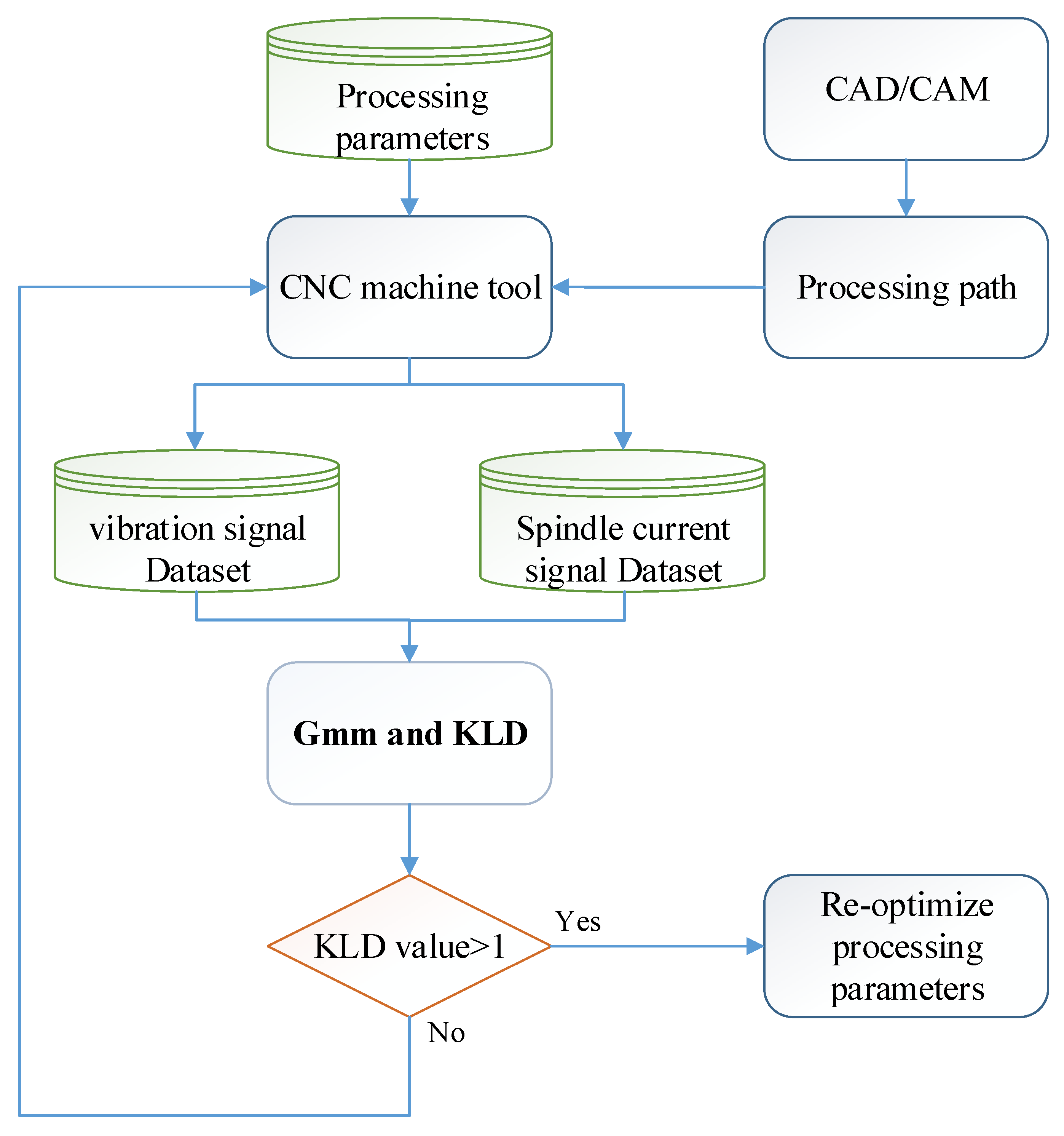
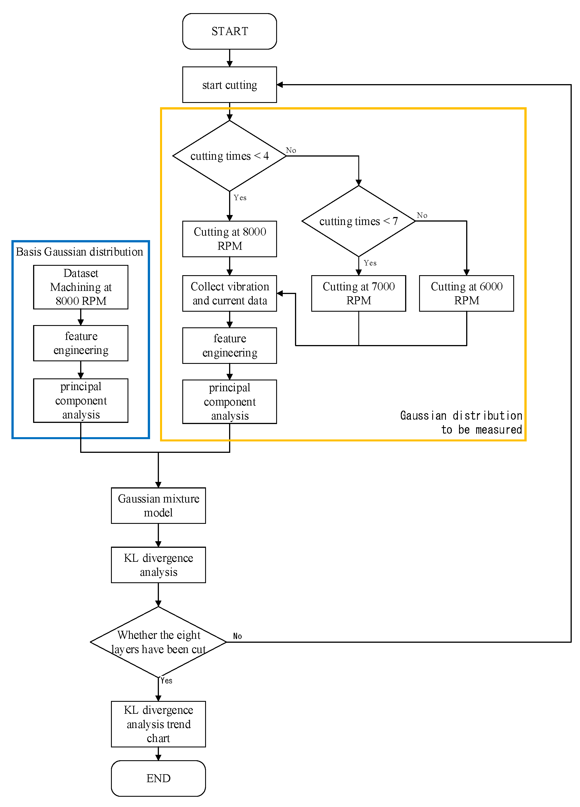
2. Research Methods
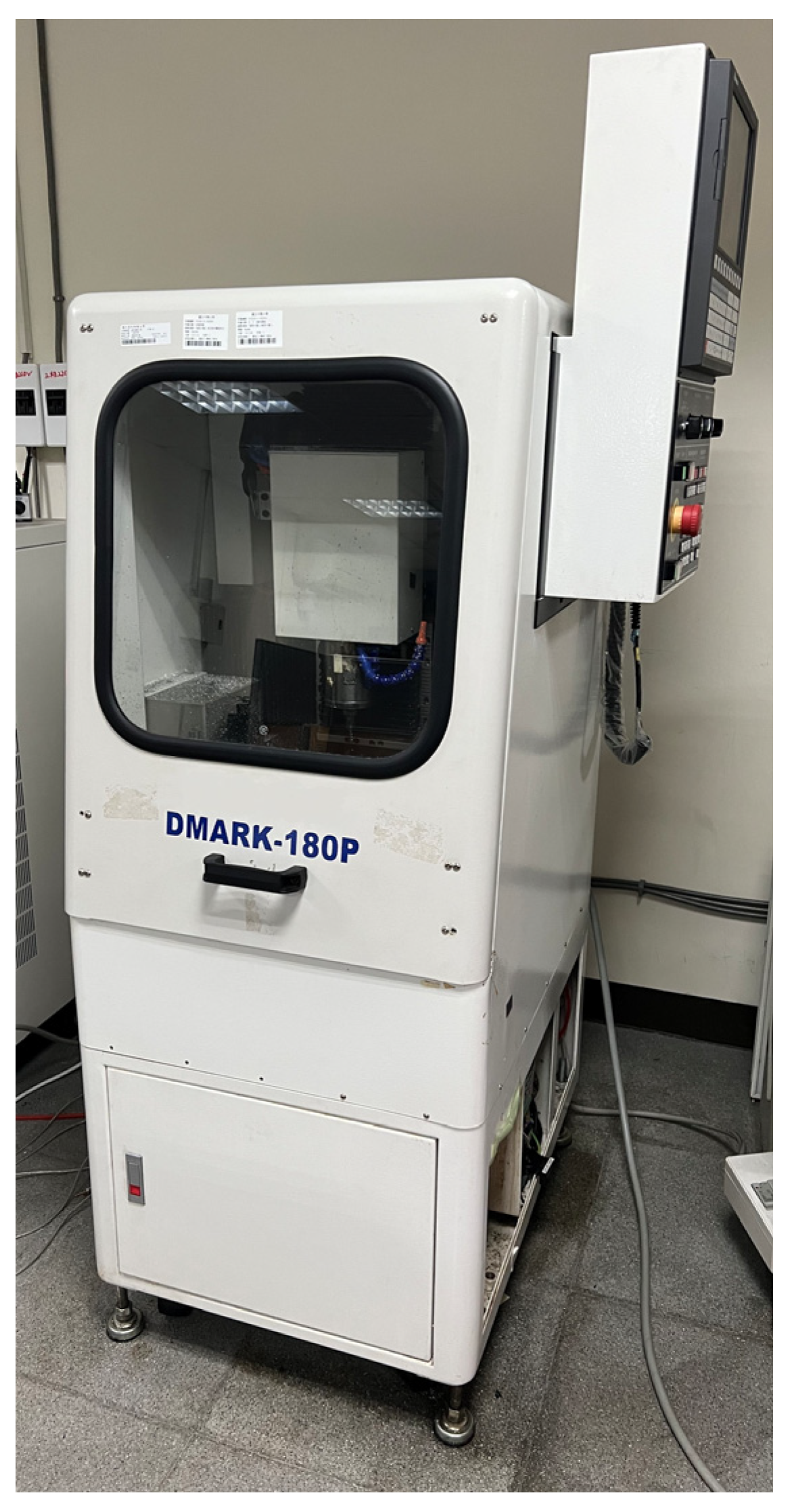
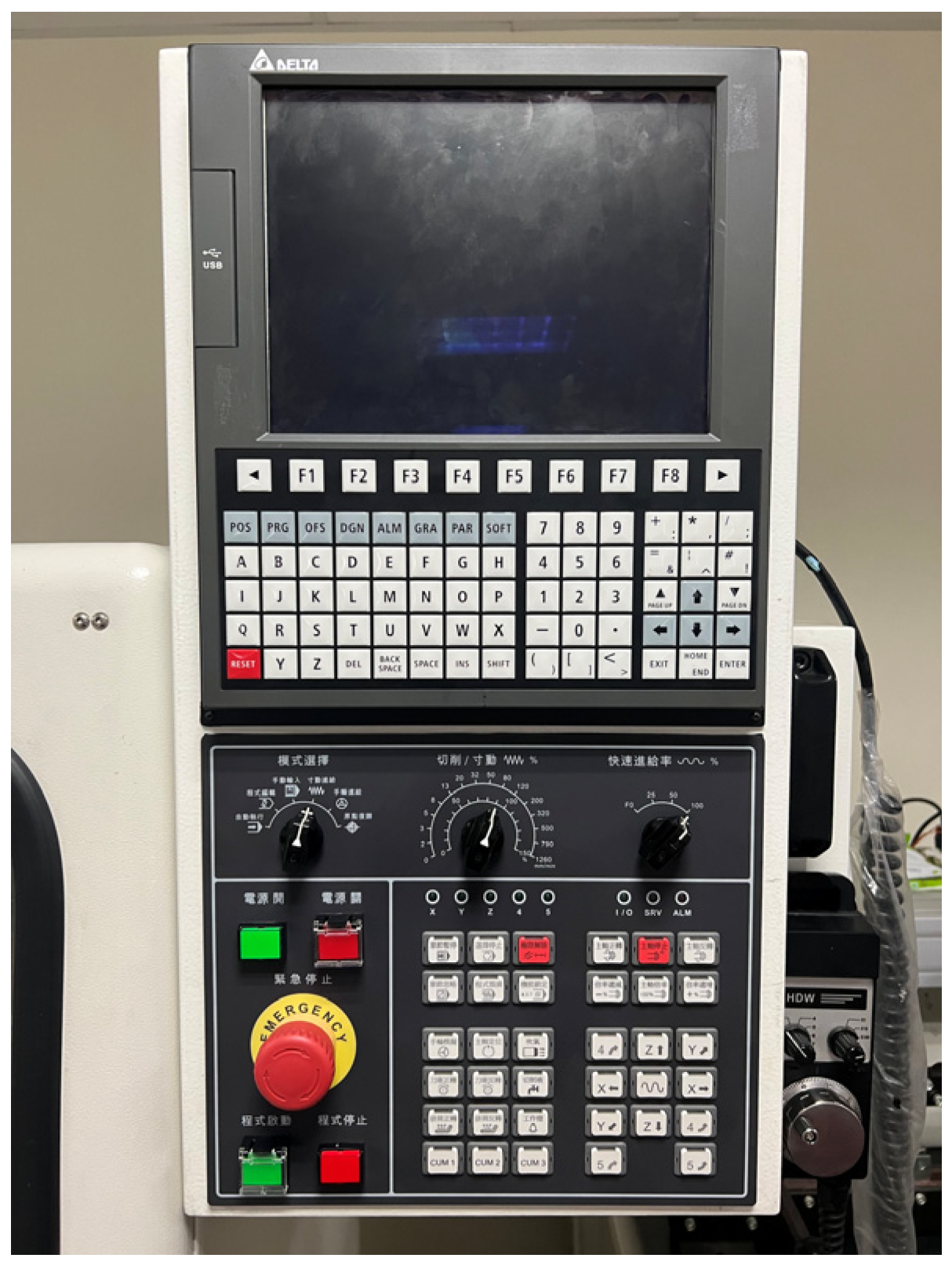
2.1. Experimental Machine
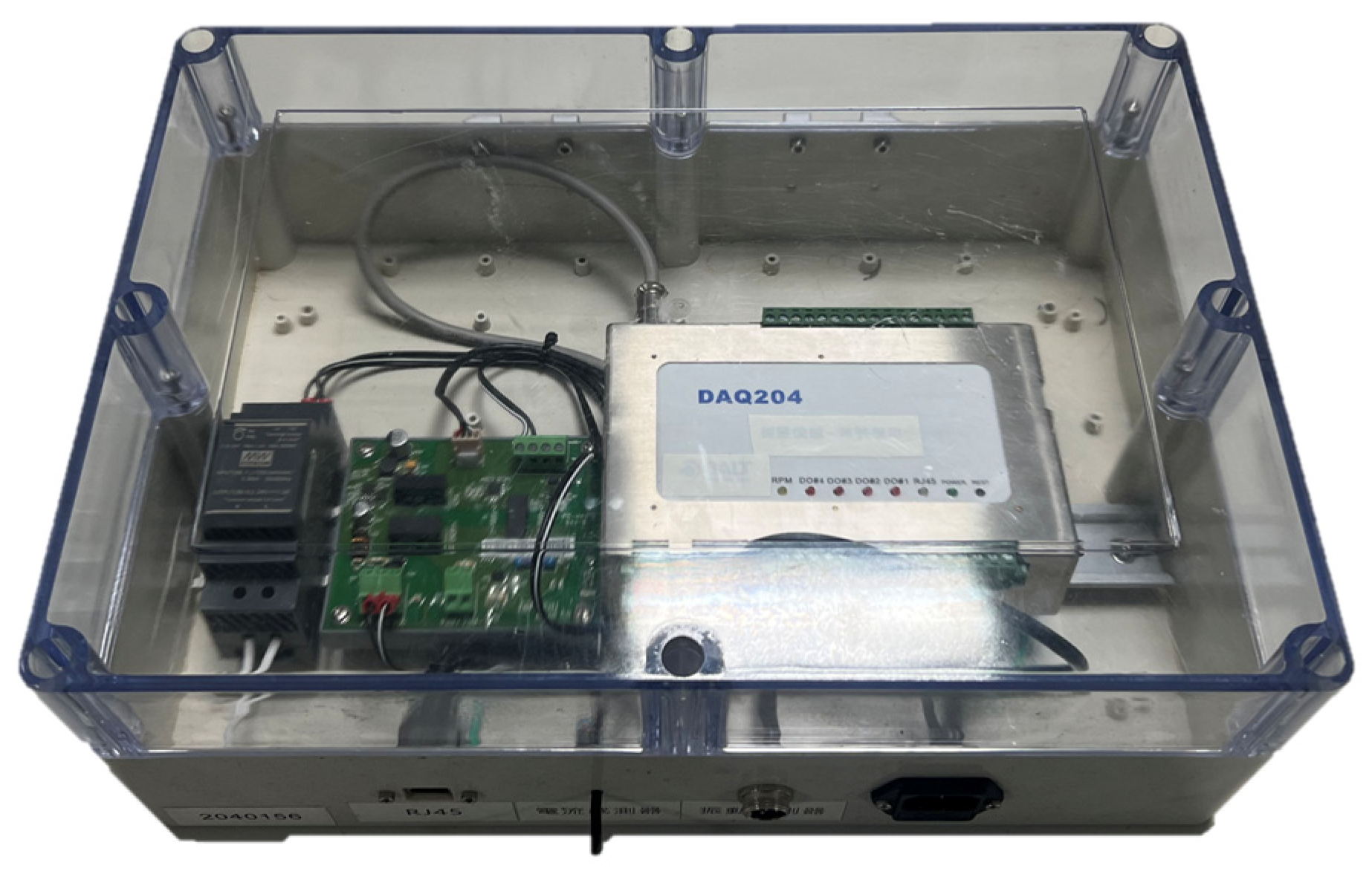
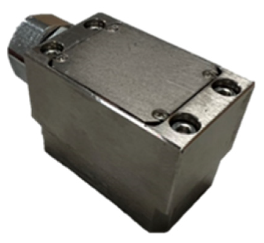
2.2. DAQ-204 Vibration-Capture Module and Triaxial Accelerometer
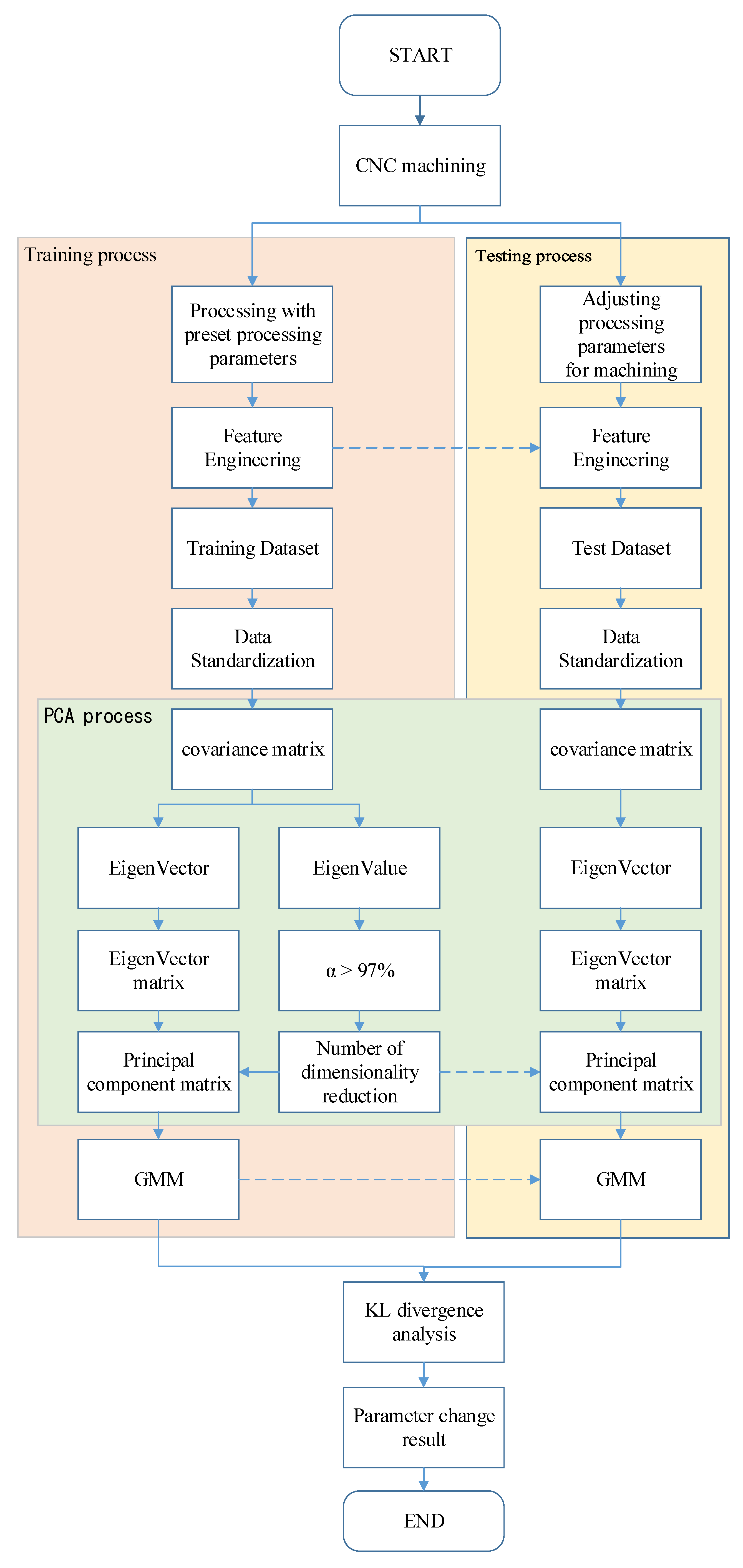
2.3. Gaussian Mixture Model
- (1)
- Expectation Step
- (2)
- Expectation Step
2.4. Feature Engineering
2.4.1. Feature Extraction
2.4.2. Outlier Reduction
2.4.3. Feature Selection
- (1)
- Standardize the raw data: Assuming that the raw data are represented by , n = 1 … N, the Z score can be described as .
- (2)
- Calculate the covariance matrix: If cov(x, y) is calculated using the feature training dataset , i = 1, 2, …, V, the covariance matrix equation is then
- (3)
- Calculate the eigenvalues and eigenvectors of the covariance matrix: in order of greatest to smallest, the eigenvalues of the covariance matrix are , i = 1 … n, and the corresponding eigenvectors are , i = 1… n.
- (4)
- Calculate the variance cumulative contribution ratio (α) of the first k principal components greater than 0.97:
- (5)
- Generate the new principal components matrix with dimensionality k:
2.5. Kullback–Leibler Divergence
2.6. F-Sscore
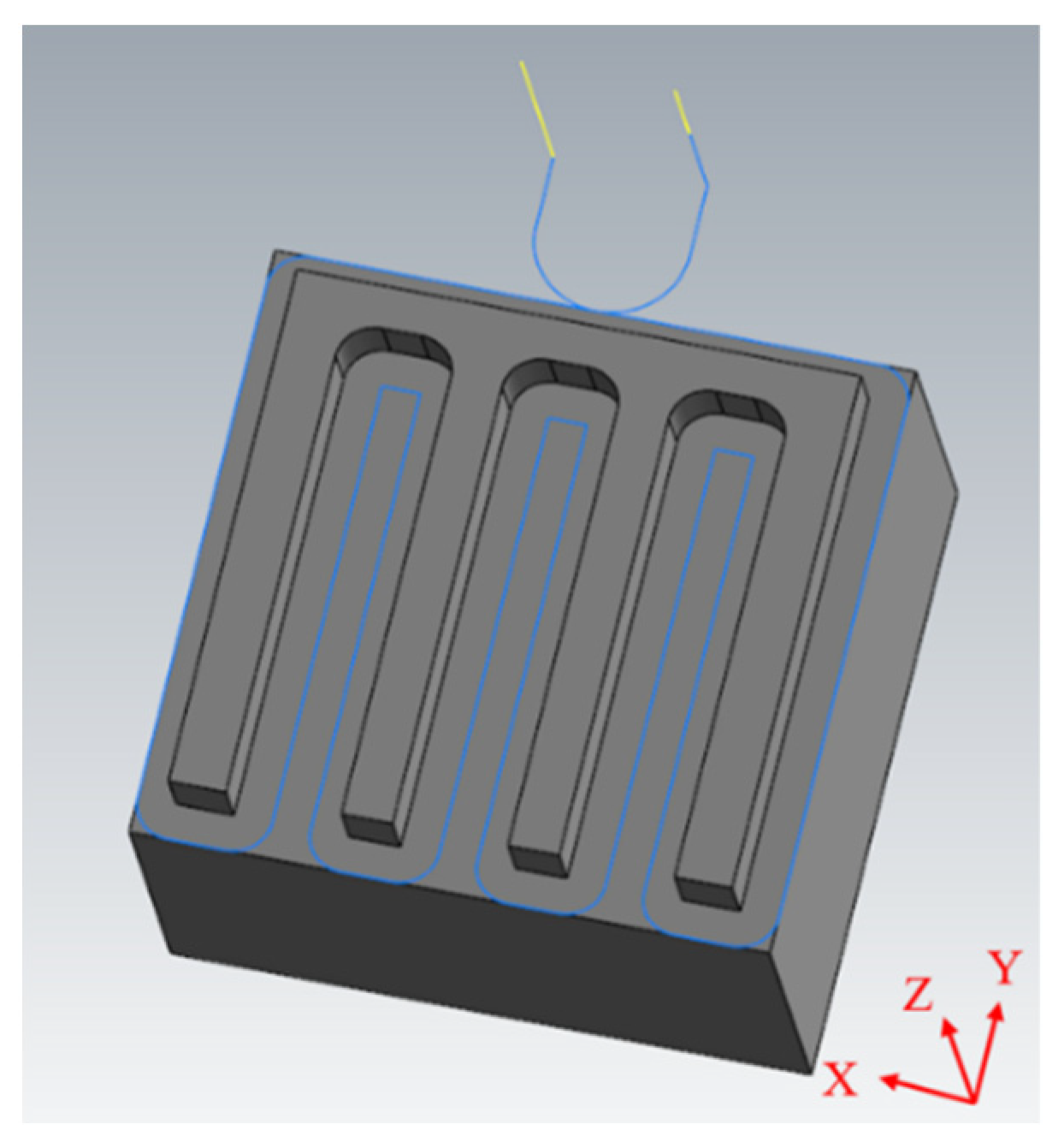
3. Experiments
4. Results and Discussion
4.1. Feature Engineering, PCA, and F-Score
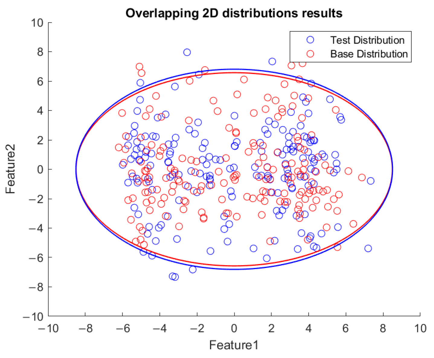
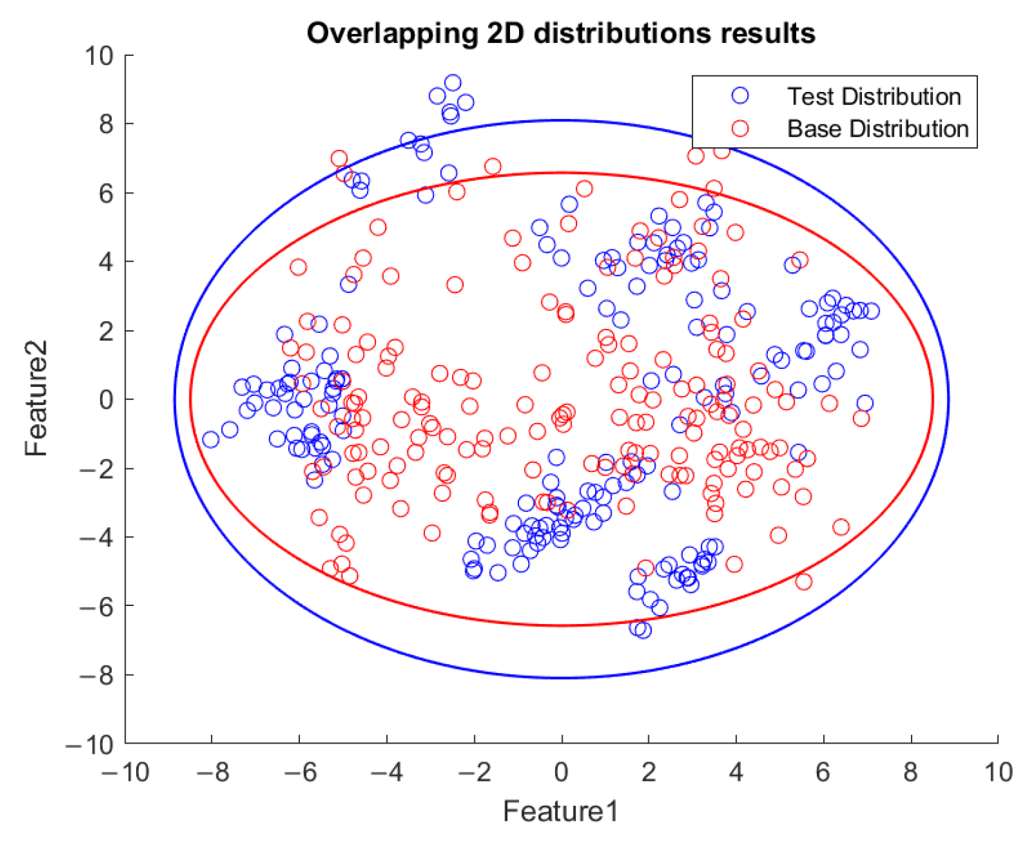
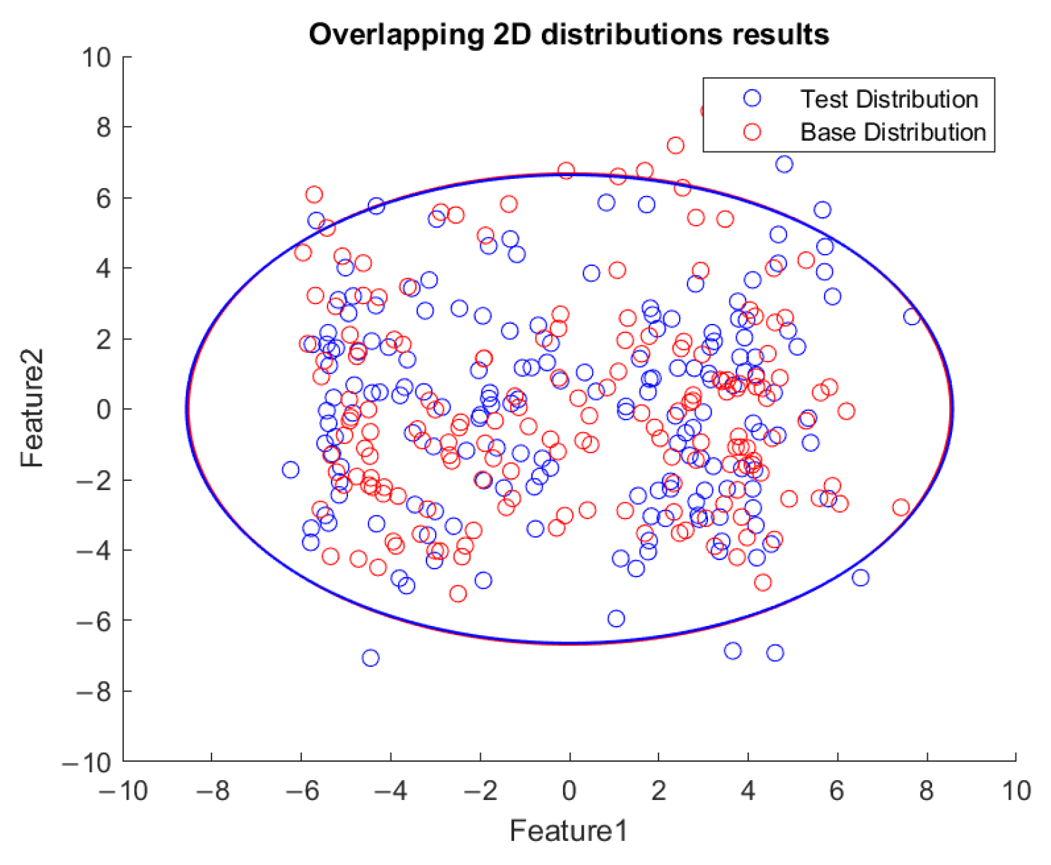
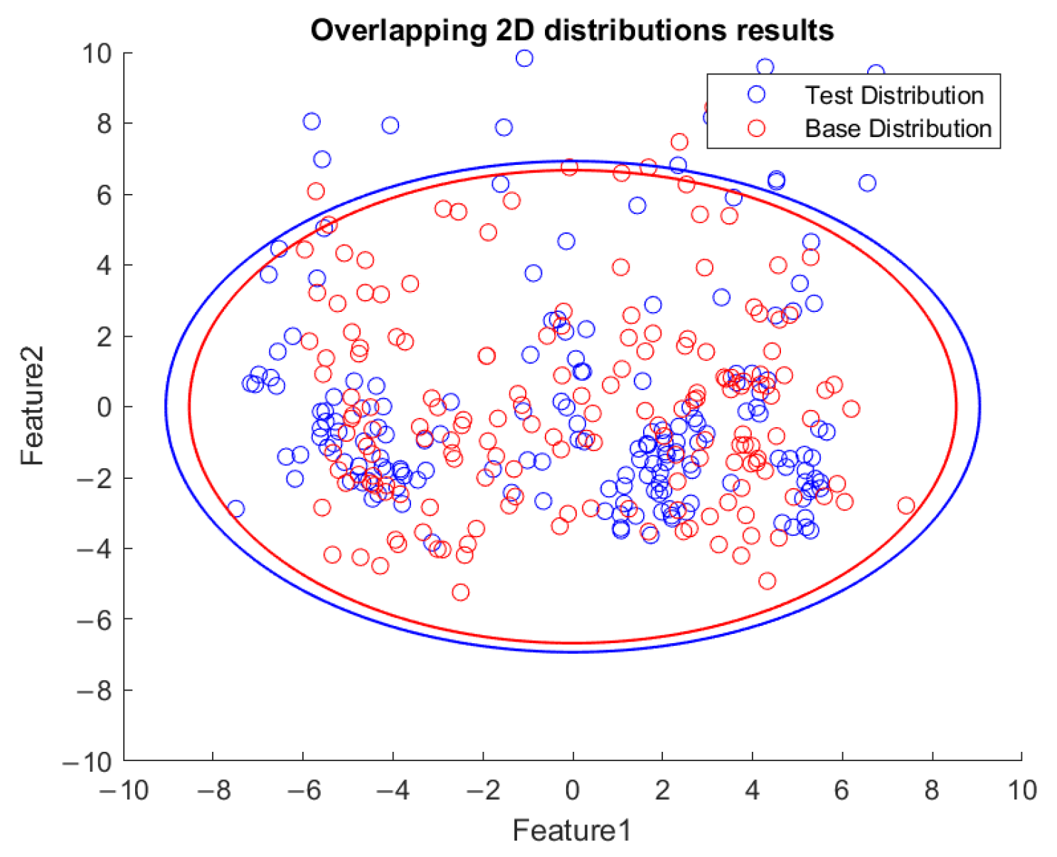
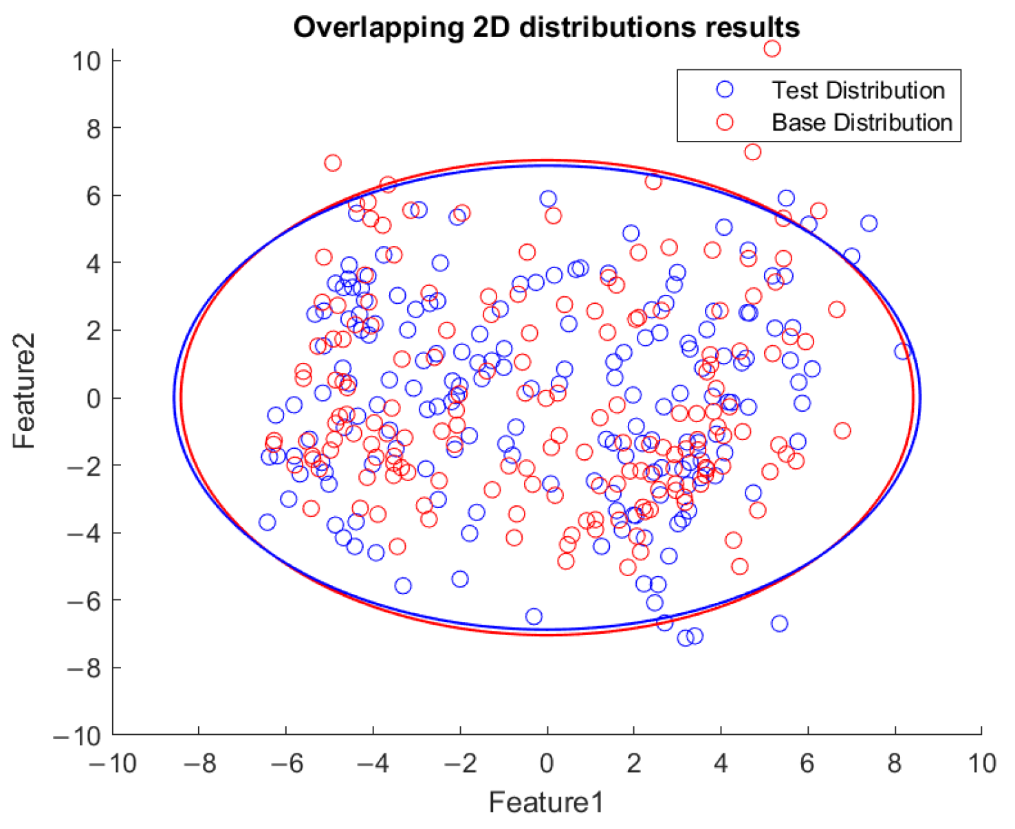
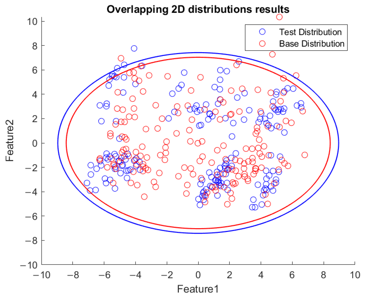
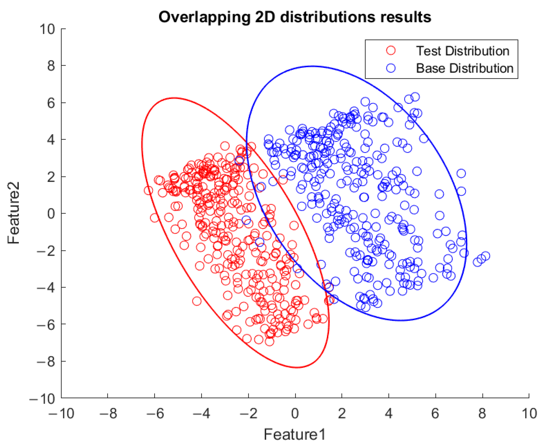
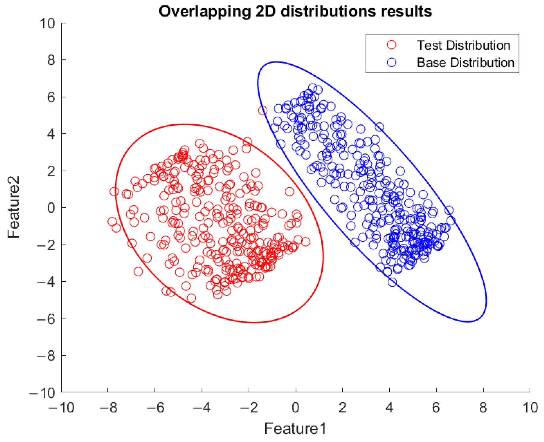
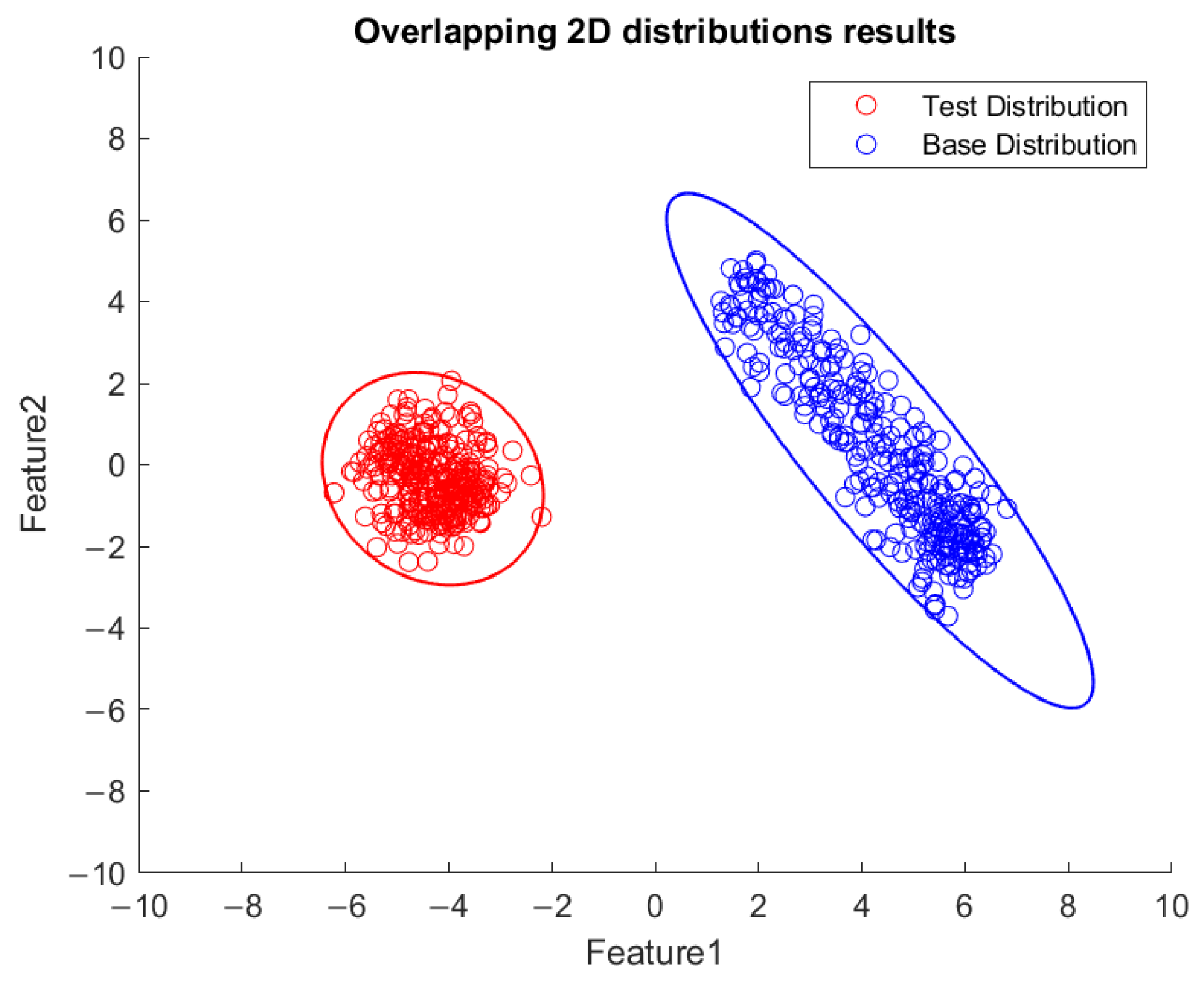
4.2. GMM Modeling and Visualization
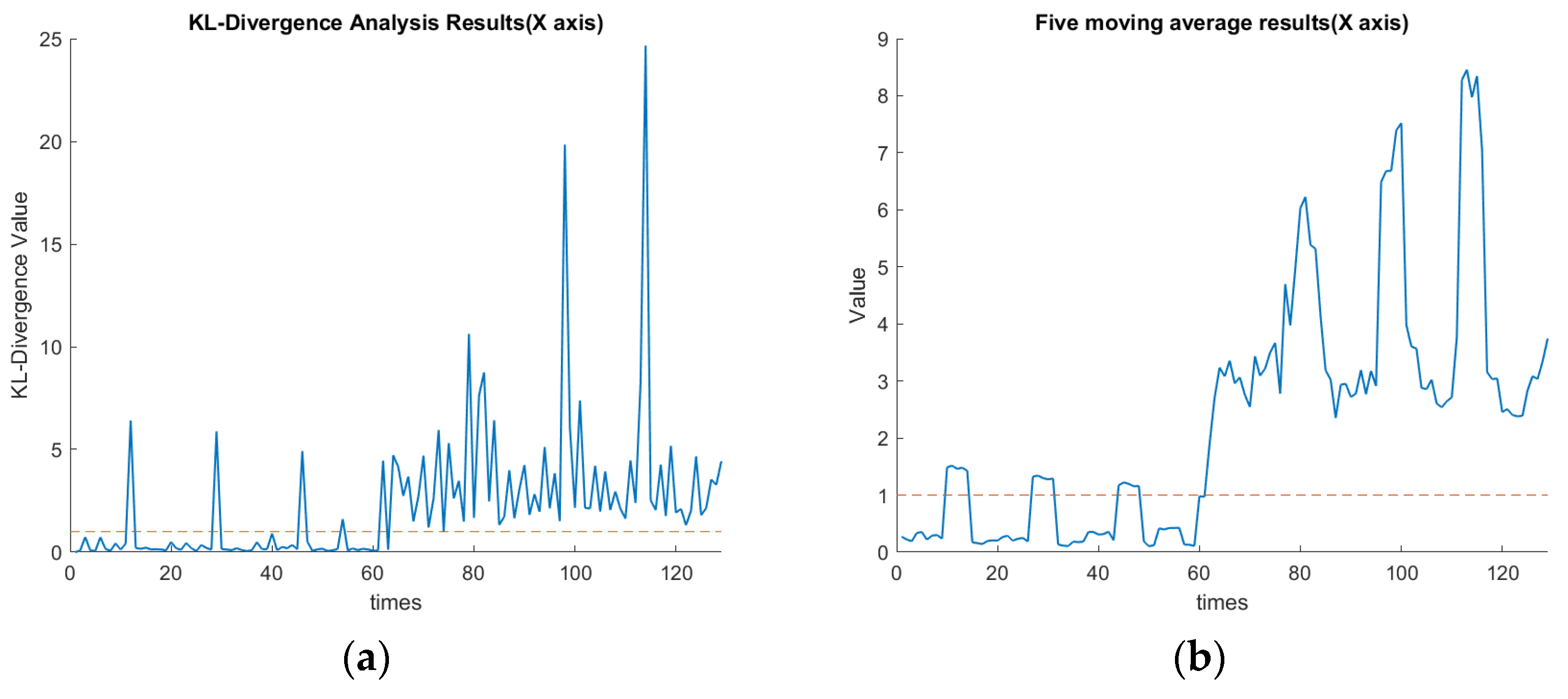
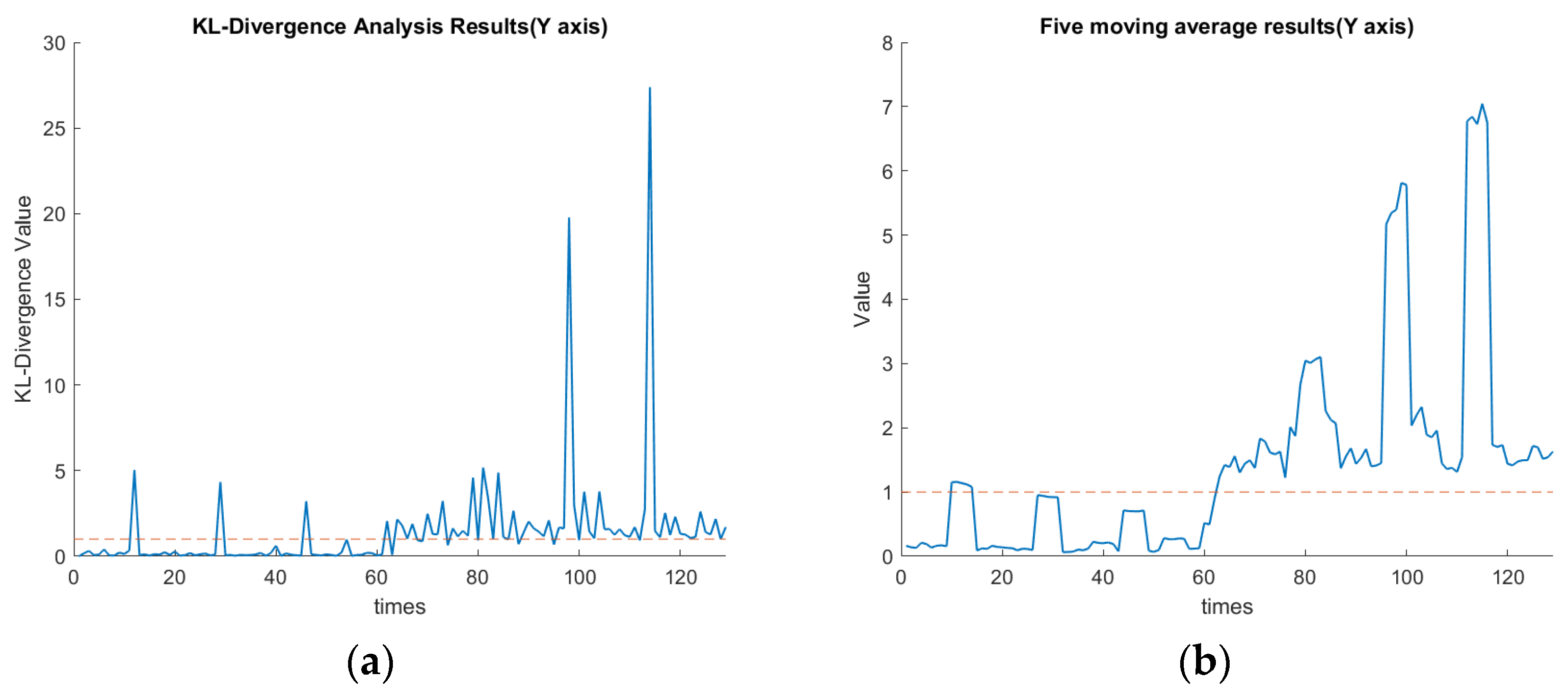
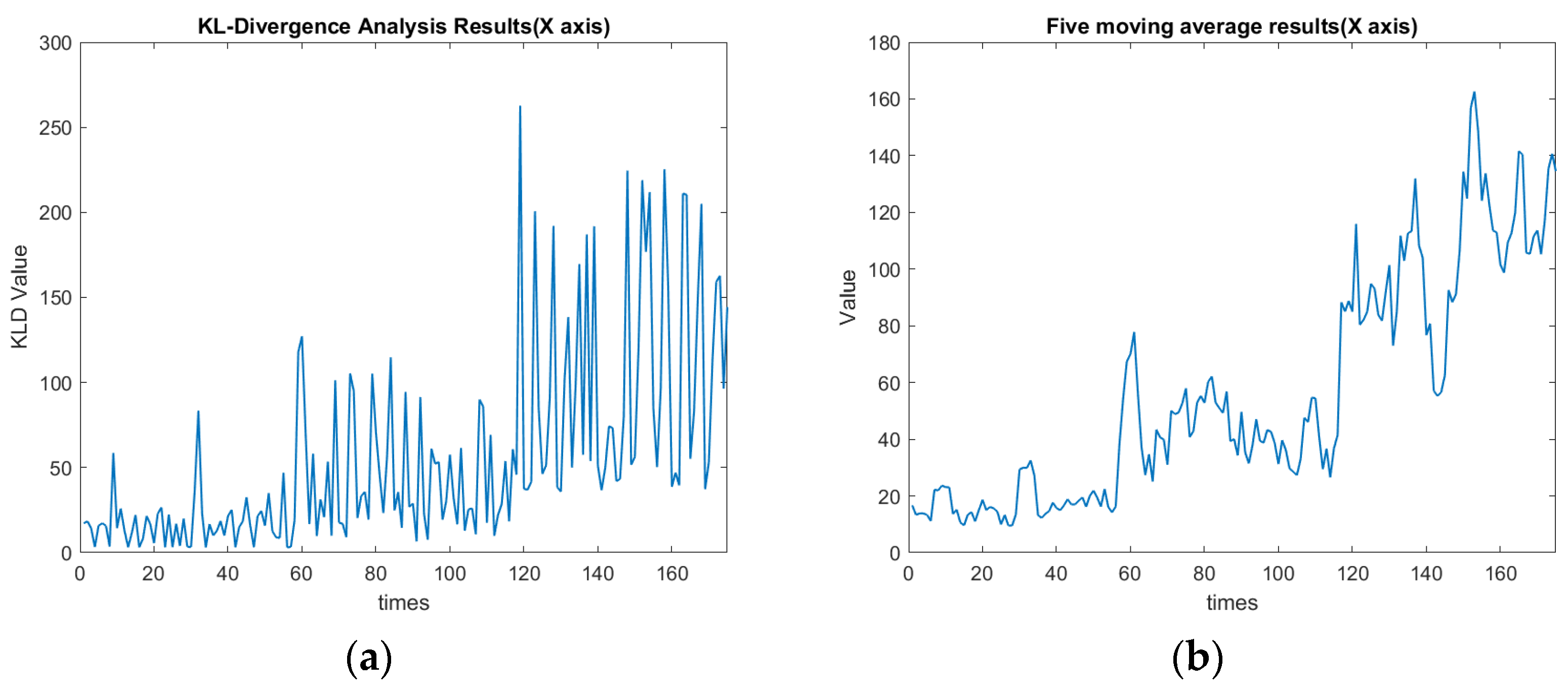
4.3. KLD and KLD’s Five-Point Moving Average
5. Conclusions
Author Contributions
Funding
Data Availability Statement
Conflicts of Interest
References
- Chiu, H.-W.; Lee, C.-H. Intelligent Machining System Based on CNC Controller Parameter Selection and Optimization. IEEE Access 2020, 8, 51062–51070. [Google Scholar] [CrossRef]
- Tsai, M.-S.; Tseng, H.-C.; Cheng, C.-C.; Li, C.-J. Optimization of Computer Numerical Control Interpolation Parameters Using a Backpropagation Neural Network and Genetic Algorithm with Consideration of Corner Vibrations. Appl. Sci. 2021, 11, 1665. [Google Scholar]
- Huang, Y.-C.; Liao, H.-S. Building prediction model for a machine tool with genetic algorithm optimization on a general regression neural network. J. Intell. Fuzzy Syst. 2020, 38, 2347–2357. [Google Scholar] [CrossRef]
- Azamfar, M.; Li, X.; Lee, J. Intelligent ball screw fault diagnosis using a deep domain adaptation methodology. Mech. Mach. Theory 2020, 151, 103932. [Google Scholar] [CrossRef]
- Lin, S.C.; Su, S.F.; Huang, Y. Smart Machine Box with Early Failure Detection for Automatic Tool Changer Subsystem of CNC Machine Tool in the Production Line. In Proceedings of the IECON 2021—47th Annual Conference of the IEEE Industrial Electronics Society, Toronto, ON, Canada, 13–16 October 2021. [Google Scholar]
- Li, G.; Fu, Y.; Chen, D.; Shi, L.; Zhou, J. Deep Anomaly Detection for CNC Machine Cutting Tool Using Spindle Current Signals. Sensors 2020, 20, 4896. [Google Scholar] [CrossRef] [PubMed]
- Irgat, E.; Çinar, E.; Ünsal, A. The detection of bearing faults for induction motors by using vibration signals and machine learning. In Proceedings of the IEEE 13th International Symposium on Diagnostics for Electrical Machines, Power Electronics and Drives, Virtual Conference, 22–25 August 2021; pp. 447–453. [Google Scholar]
- Wang, R.; Song, Q.; Liu, Z.; Ma, H.; Gupta, M.K.; Liu, Z. A Novel Unsupervised Machine Learning-Based Method for Chatter Detection in the Milling of Thin-Walled Parts. Sensors 2021, 21, 5779. [Google Scholar] [CrossRef] [PubMed]
- Dou, J.; Xu, C.; Jiao, S.; Li, B.; Zhang, J.; Xu, X. An unsupervised online monitoring method for tool wear using a sparse auto-encoder. Int. J. Adv. Manuf. Technol. 2020, 106, 2493–2507. [Google Scholar] [CrossRef]
- Hong, Y.; Kim, M.; Lee, H.; Park, J.J.; Lee, D. Early Fault Diagnosis and Classification of Ball Bearing Using Enhanced Kurtogram and Gaussian Mixture Model. IEEE Trans. Instrum. Meas. 2019, 68, 4746–4755. [Google Scholar] [CrossRef]
- Wang, Q.; Ma, S.; Yue, D. Identification of damage in composite structures using Gaussian mixture model-processed Lamb waves. Smart Mater. Struct. 2018, 27, 045007. [Google Scholar] [CrossRef]
- Guo, Y.; Chen, H. Fault diagnosis of VRF air-conditioning system based on improved Gaussian mixture model with PCA approach. Int. J. Refrig. 2020, 118, 1–11. [Google Scholar] [CrossRef]
- Yu, J. Fault Detection Using Principal Components-Based Gaussian Mixture Model for Semiconductor Manufacturing Processes. IEEE Trans. Semicond. Manuf. 2011, 24, 432–444. [Google Scholar] [CrossRef]
- Liu, W.; Cui, D.; Peng, Z.; Zhong, J. Outlier Detection Algorithm Based on Gaussian Mixture Model. In Proceedings of the 2019 IEEE International Conference on Power, Intelligent Computing and Systems (ICPICS), Shenyang, China, 12–14 July 2019. [Google Scholar]
- He, M.; Guo, W. An Integrated Approach for Bearing Health Indicator and Stage Division Using Improved Gaussian Mixture Model and Confidence Value. IEEE Trans. Ind. Inform. 2022, 18, 5219–5230. [Google Scholar] [CrossRef]
- Nam, J.S.; Kwon, W.T. A Study on Tool Breakage Detection During Milling Process Using LSTM-Autoencoder and Gaussian Mixture Model. Int. J. Precis. Eng. Manuf. 2022, 23, 667–675. [Google Scholar] [CrossRef]
- He, Z.; Zhang, X.; Liu, C.; Han, T. Fault Prognostics for Photovoltaic Inverter Based on Fast Clustering Algorithm and Gaussian Mixture Model. Energies 2020, 13, 4901. [Google Scholar] [CrossRef]
- Lucà, F.; Manzoni, S.; Cerutti, F.; Cigada, A. A Damage Detection Approach for Axially Loaded Beam-like Structures Based on Gaussian Mixture Model. Sensors 2022, 22, 8336. [Google Scholar] [CrossRef]
- Maliuk, A.S.; Prosvirin, A.E.; Ahmad, Z.; Kim, C.H.; Kim, J.-M. Novel Bearing Fault Diagnosis Using Gaussian Mixture Model-Based Fault Band Selection. Sensors 2021, 21, 6579. [Google Scholar] [CrossRef]
- Zhang, B.; Yan, X.; Liu, G.; Fan, K. Multi-source fault diagnosis of chiller plant sensors based on an improved ensemble empirical mode decomposition Gaussian mixture model. Energy Rep. 2022, 8, 2831–2842. [Google Scholar] [CrossRef]
- Lu, C.; Wang, S. Performance Degradation Prediction Based on a Gaussian Mixture Model and Optimized Support Vector Regression for an Aviation Piston Pump. Sensors 2020, 20, 3854. [Google Scholar] [CrossRef]
- Yu, J. Machine Tool Condition Monitoring Based on an Adaptive Gaussian Mixture Model. J. Manuf. Sci. Eng. 2012, 134, 031004. [Google Scholar] [CrossRef]
- Chen, H.; Jiang, B.; Lu, N. An improved incipient fault detection method based on Kullback-Leibler divergence. ISA Trans. 2018, 79, 127–136. [Google Scholar] [CrossRef]
- Cao, Y.; Jan, N.M.; Huang, B.; Wang, Y.; Gui, W. No-Delay Multimodal Process Monitoring Using Kullback-Leibler Divergence-Based Statistics in Probabilistic Mixture Models. IEEE Trans. Autom. Sci. Eng. 2023, 20, 167–178. [Google Scholar] [CrossRef]
- Huang, C.-R.; Lu, M.-C. Investigation of Cutting Path Effect on Spindle Vibration and AE Signal Features for Tool Wear Monitoring in Micro Milling. Appl. Sci. 2023, 13, 1107. [Google Scholar] [CrossRef]
- Jiang, D.; Li, W.; Shen, F. Incipient fault diagnosis and amplitude estimation based on K–L divergence with a Gaussian mixture model. Rev. Sci. Instrum. 2020, 91, 055103. [Google Scholar] [CrossRef] [PubMed]
- Hotelling, H. Analysis of a Complex of Statistical Variables with Principal Components. J. Educ. Psychol. 1933, 24, 417–441. [Google Scholar] [CrossRef]
- Tra, V.; Amayri, M.; Bouguila, N. Outlier detection via multiclass deep autoencoding Gaussian mixture model for building chiller diagnosis. Energy Build. 2022, 259, 111893. [Google Scholar] [CrossRef]


| Spindle | Speed | 24,000 rpm (max), 2.2 kW |
| Motor | Built-in | |
| Cooling | Cold air | |
| Servo motor | x-axis | 400 W |
| y-axis | 400 W | |
| z-axis | 400 W | |
| Servo drive | A2, 400 W, single-phase/three-phase connections | |
| Travel | x-axis | 160 mm |
| y-axis | 180 mm | |
| z-axis | 150 mm | |
| Feed | Rapid movement (G0) | Maximum x-,y-, and z-axis speeds: 6/6/6 m/min |
| Control precision (controller) | 0.001 mm | |
| Machine body | Length | 750 mm |
| Width | 500 mm | |
| Height | 1400 mm | |
| Control | Control format | Standard G code, standard M code |
| Connection modes | ETHERNET/USB | |
| Input channels | 2/4 channels |
| IEPE | ±10 V |
| Maximum sampling frequency | 102,400 Hz |
| Bandwidth range | 12.8 kHz |
| Model | BT-1513 |
| Acceleration range | ±50 g |
| Bandwidth | 0.5–15 kHz |
| Triaxial sensitivity | X: 108.85 mV/g |
| Y: 100.48 mV/g | |
| Z: 103.64 mV/g |
| Total Data of 25,600 (Vibration Value) + 25,600 (Current Value) in One Data Segment | ||
|---|---|---|
| Order | Feature | Sensing Data |
| 1 | RMS | vibration value |
| 2 | Kurtosis | |
| 3 | Variance | |
| 4 | Crest Factor | |
| 5 | Standard deviation | |
| 6 | Skewness | |
| 7–22 | Average amplitude of frequency sectors [1 + 400 × (i − 1)] Hz~(400 × i) Hz, i = 1,2,3,…,16 | |
| 23–38 | Average amplitude of frequency sectors [1 + 400 × (i − 1)] Hz~(400 × i) Hz, i = 1,2,3,…,16 | current value |
| 39 | PSD-Amplitude Mean | vibration value |
| 40 | PSD-Amplitude Standard deviation | |
| 41 | PSD-Amplitude Skewness | |
| 42 | PSD-Amplitude Kurtosis | |
| 43 | PSD-Shape Mean | |
| 44 | PSD-Shape Standard deviation | |
| 45 | PSD-Shape Skewness | |
| 46 | PSD-Shape Kurtosis | |
| Before | After | ||
|---|---|---|---|
| x-axis | 200 × 46 | 200 × 23 | |
| y-axis | 200 × 46 | 200 × 23 | |
| z-axis | 200 × 46 | 200 × 23 | |
| KLD < 1 | KLD > 1 | |
|---|---|---|
| KLD < 1 (1–65th data section tests: 6000 rpm) | TP | FN |
| KLD > 1 (65th–129th data section tests: 5500 rpm) | FP | TN |
| TP | FN | FP | TN | F-Score | |
| x-axis | 58 | 6 | 0 | 65 | 0.9508 |
| y-axis | 59 | 5 | 10 | 55 | 0.8872 |
| z-axis | 59 | 5 | 4 | 61 | 0.9291 |
| 6000 RPM (1–65th Data Section) without Data Cleaning | 6000 RPM (1–65th Data Section) with Data Cleaning | 5500 RPM (65th–129th Data Section) without Data Cleaning | 5500 RPM (65th–129th Data Section) with Data Cleaning | |
|---|---|---|---|---|
| x-axis | 0.675 | 0.43 | 3.953 | 3.244 |
| y-axis | 0.409 | 0.226 | 2.448 | 1.767 |
| z-axis | 0.404 | 0.237 | 2.562 | 1.9 |
Disclaimer/Publisher’s Note: The statements, opinions and data contained in all publications are solely those of the individual author(s) and contributor(s) and not of MDPI and/or the editor(s). MDPI and/or the editor(s) disclaim responsibility for any injury to people or property resulting from any ideas, methods, instructions or products referred to in the content. |
© 2023 by the authors. Licensee MDPI, Basel, Switzerland. This article is an open access article distributed under the terms and conditions of the Creative Commons Attribution (CC BY) license (https://creativecommons.org/licenses/by/4.0/).
Share and Cite
Huang, Y.-C.; Hou, C.-C. Using Feature Engineering and Principal Component Analysis for Monitoring Spindle Speed Change Based on Kullback–Leibler Divergence with a Gaussian Mixture Model. Sensors 2023, 23, 6174. https://doi.org/10.3390/s23136174
Huang Y-C, Hou C-C. Using Feature Engineering and Principal Component Analysis for Monitoring Spindle Speed Change Based on Kullback–Leibler Divergence with a Gaussian Mixture Model. Sensors. 2023; 23(13):6174. https://doi.org/10.3390/s23136174
Chicago/Turabian StyleHuang, Yi-Cheng, and Ching-Chen Hou. 2023. "Using Feature Engineering and Principal Component Analysis for Monitoring Spindle Speed Change Based on Kullback–Leibler Divergence with a Gaussian Mixture Model" Sensors 23, no. 13: 6174. https://doi.org/10.3390/s23136174
APA StyleHuang, Y.-C., & Hou, C.-C. (2023). Using Feature Engineering and Principal Component Analysis for Monitoring Spindle Speed Change Based on Kullback–Leibler Divergence with a Gaussian Mixture Model. Sensors, 23(13), 6174. https://doi.org/10.3390/s23136174