


Data Fusion for Cross-Domain Real-Time Object Detection on the Edge


Abstract
1. Introduction
2. Related Work
2.1. Robot Control in Edge or Cloud
2.2. Interaction
2.3. Inspection
2.4. Object Detection
2.5. Multi-Task CNN
2.6. Model Pruning
2.7. Optimizing Image-Processing Queues in Edge Clouds
2.8. Optimization of CNNs for Cloud Computing
3. System Architecture
4. Experimental Setup
4.1. Datasets
4.1.1. Our Datasets
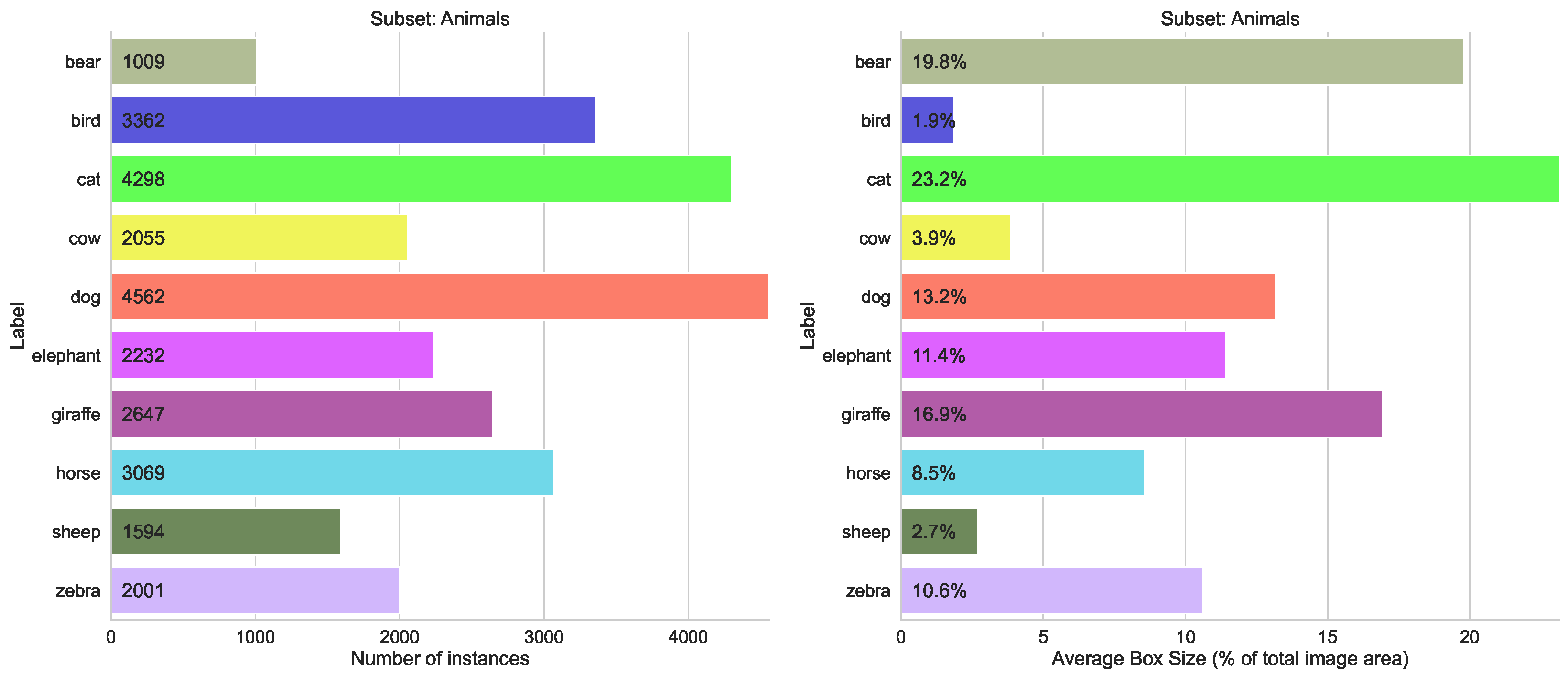
4.1.2. Generalized Dataset
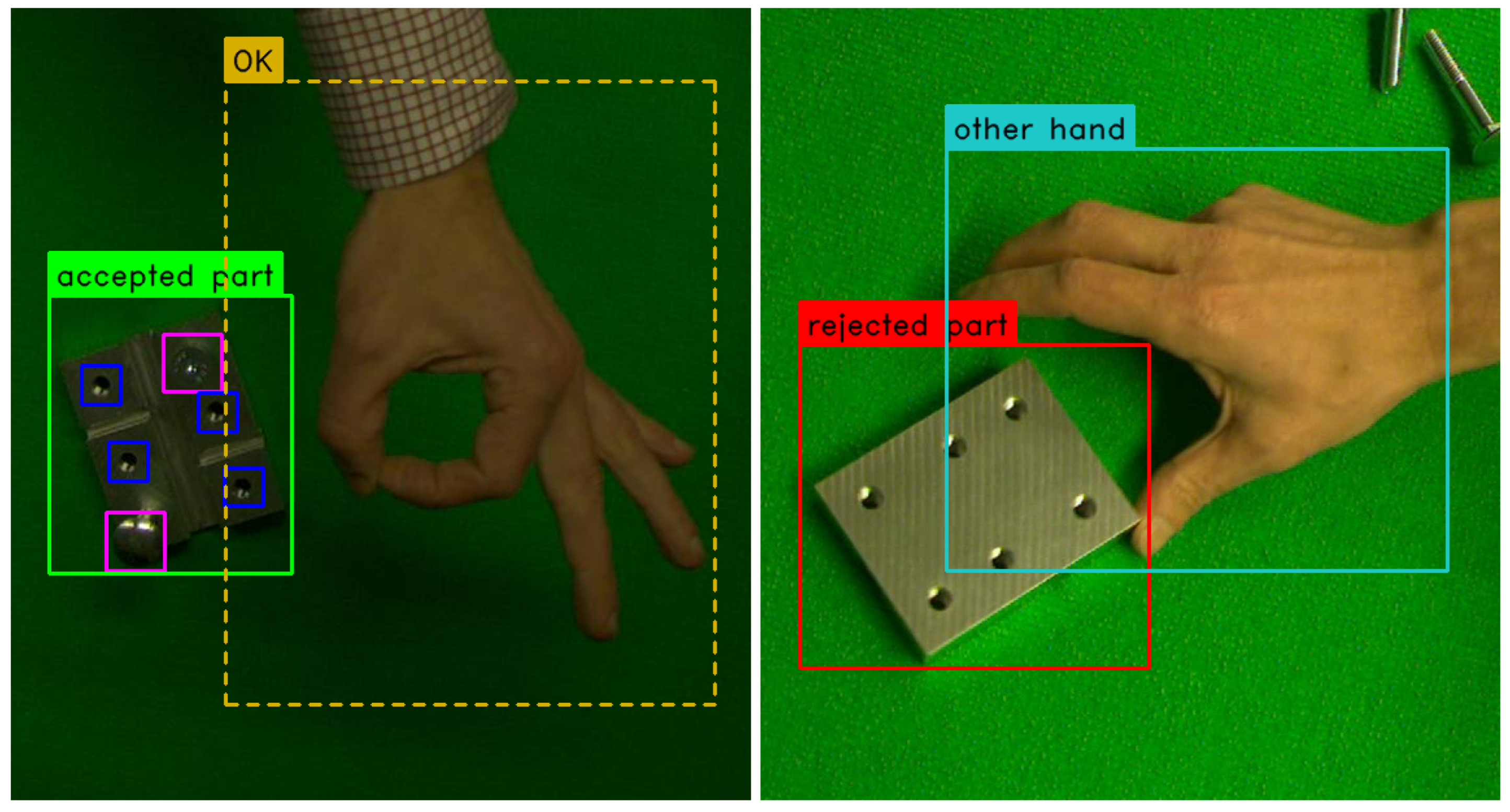
- different knowledge domains, when merging a dataset containing metallic construction pieces with screws and bots with a dataset containing human hand gestures;
- vastly different object sizes, with screw holes taking up less than of the total image area, and hand gestures—up to ;
- unbalanced number of instances per label, where every construction piece always has six times as many screws/holes, the “other gesture” class dominates the hand dataset, and the small number of “rejected part” instances
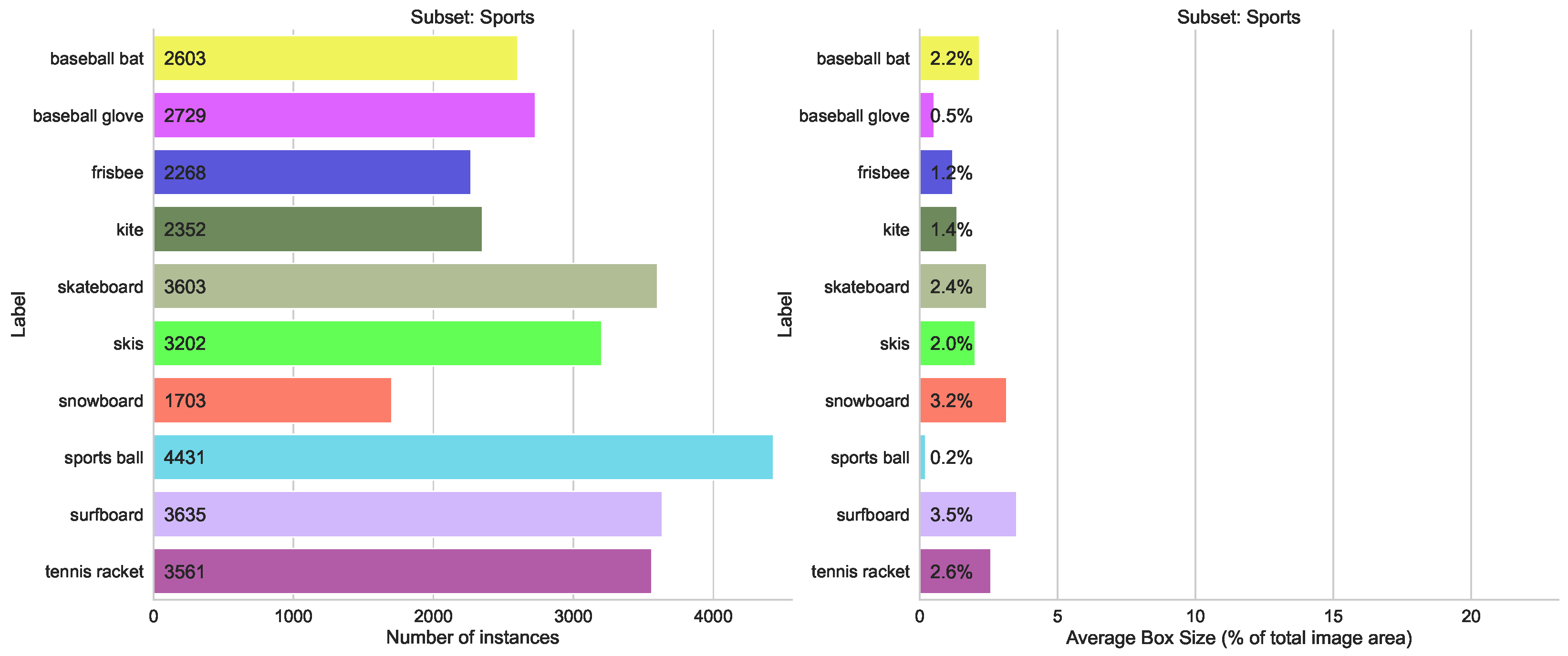
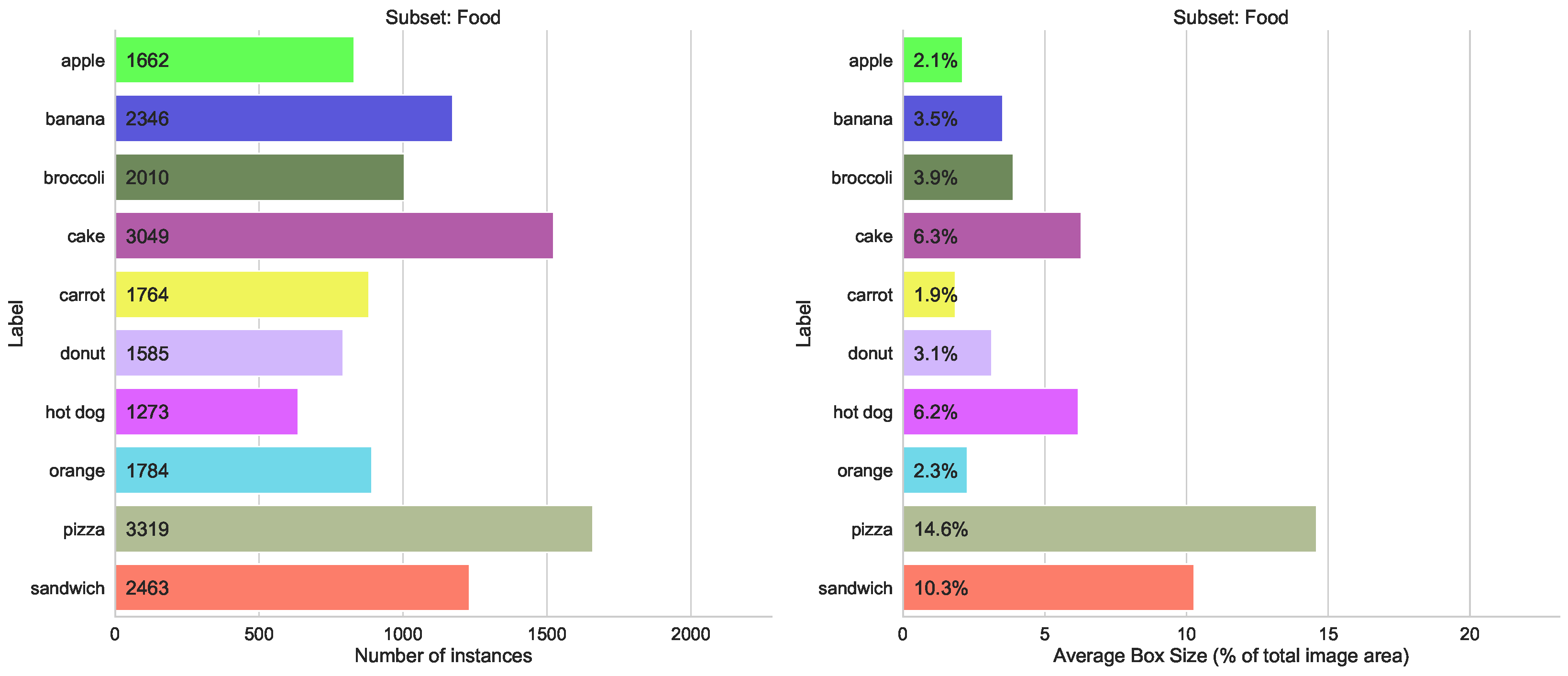
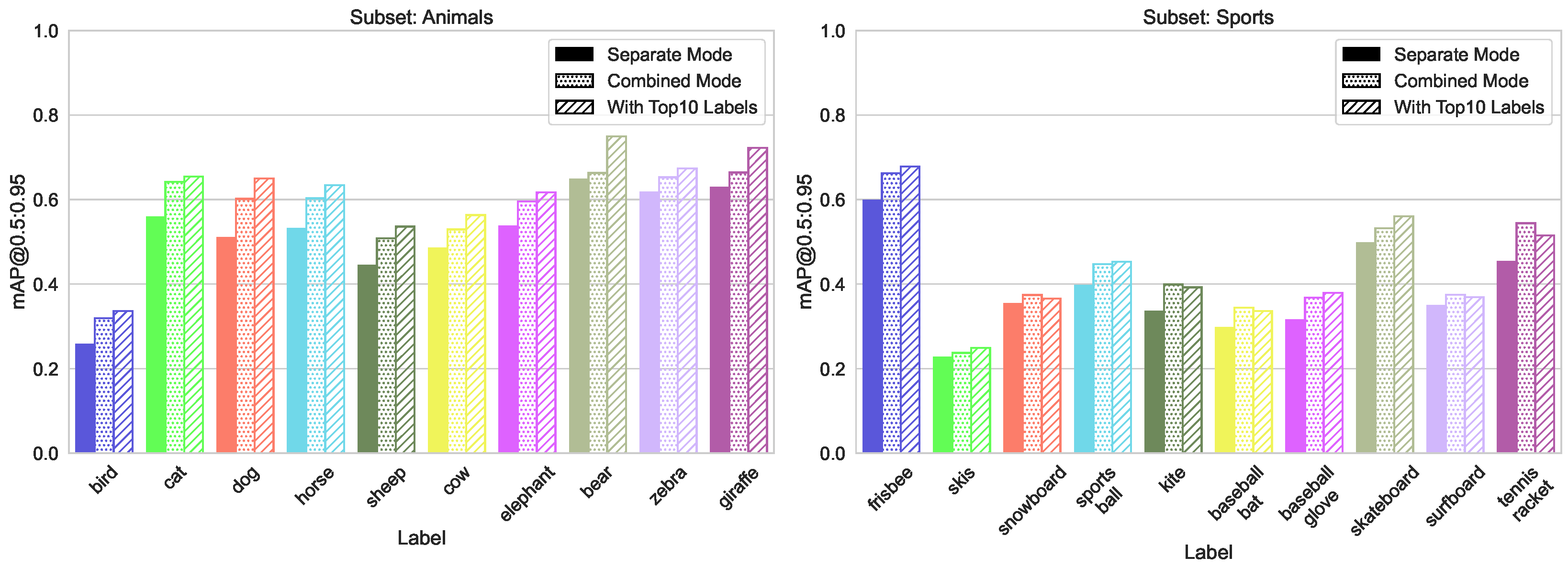
- Domains split, containing three subsets “Animals”, “Food” and “Sport”, with 10 classes in each, with a similar distribution of the number of labeled instances
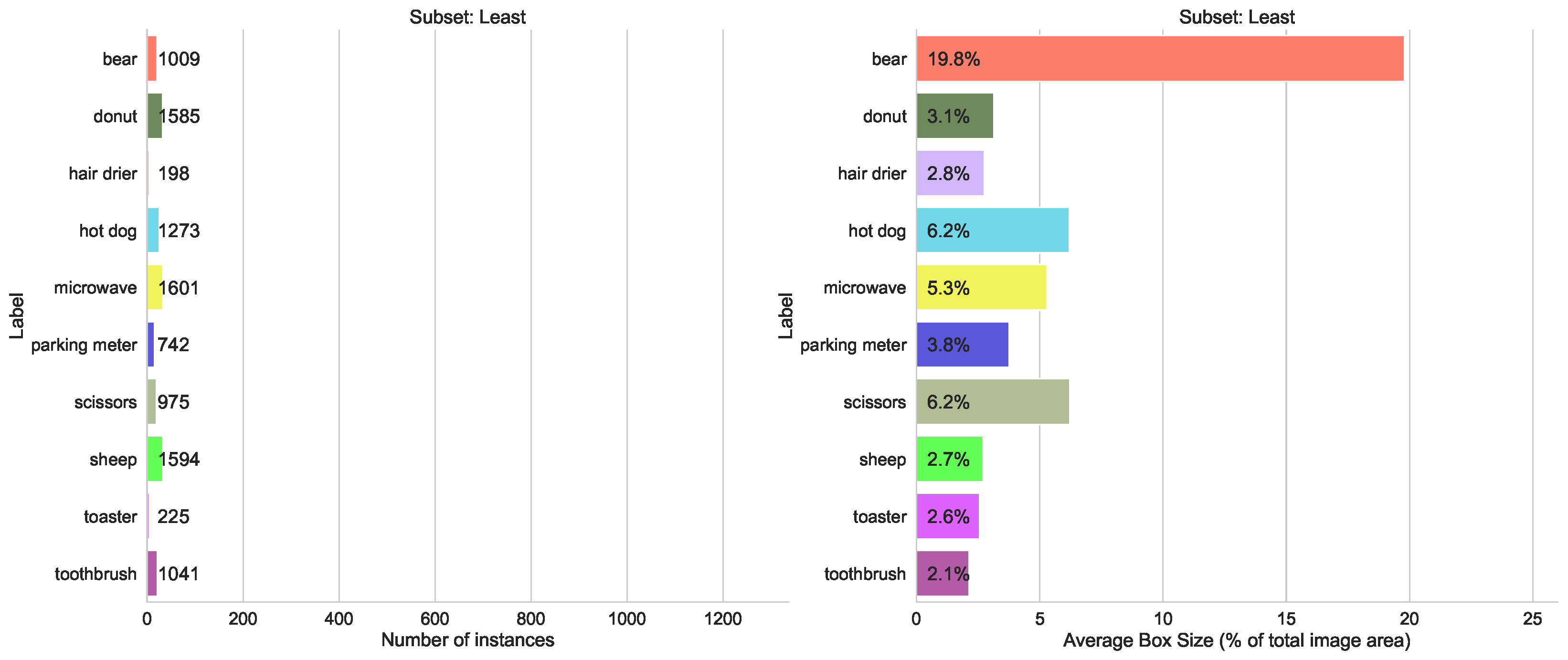
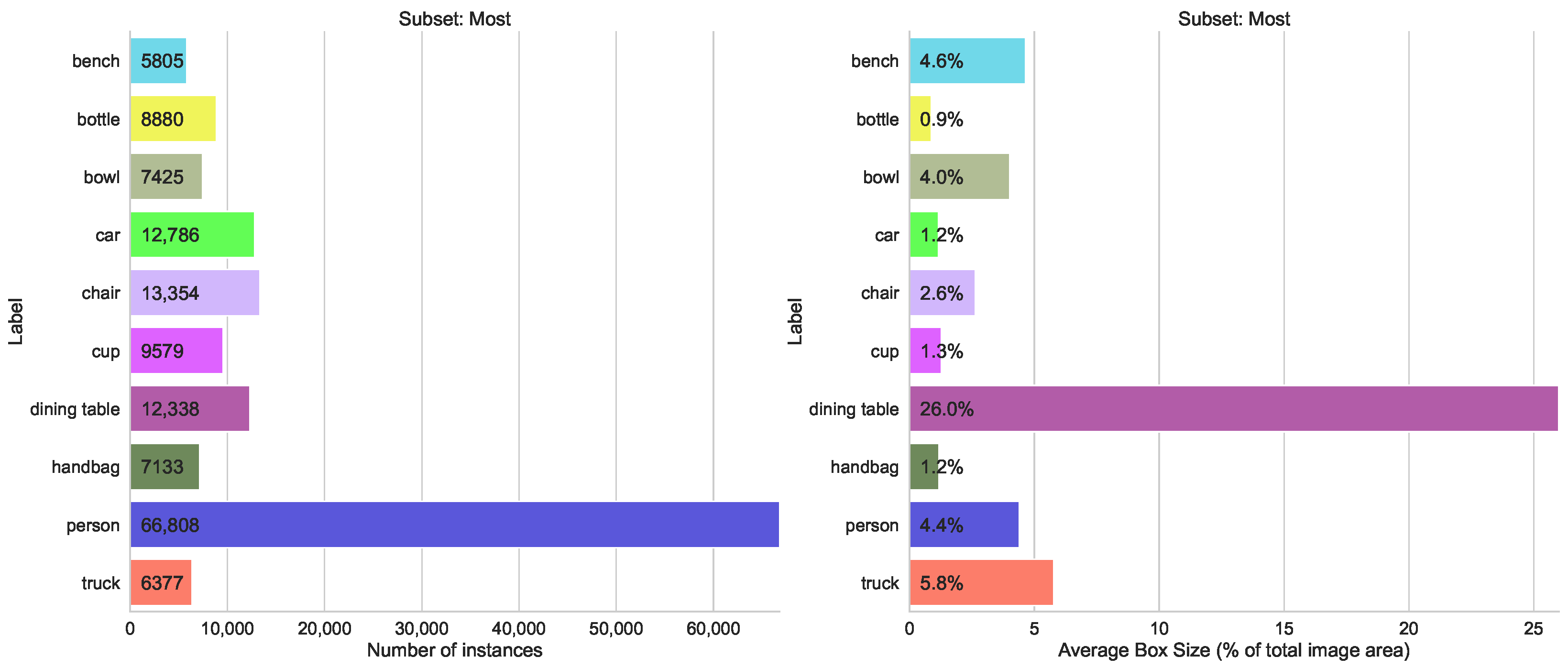
- Number of Instances per Labels split, containing two subsets—one with the top 10 classes that have the highest number of labeled instances, and another with the 10 classes that have the lowest number
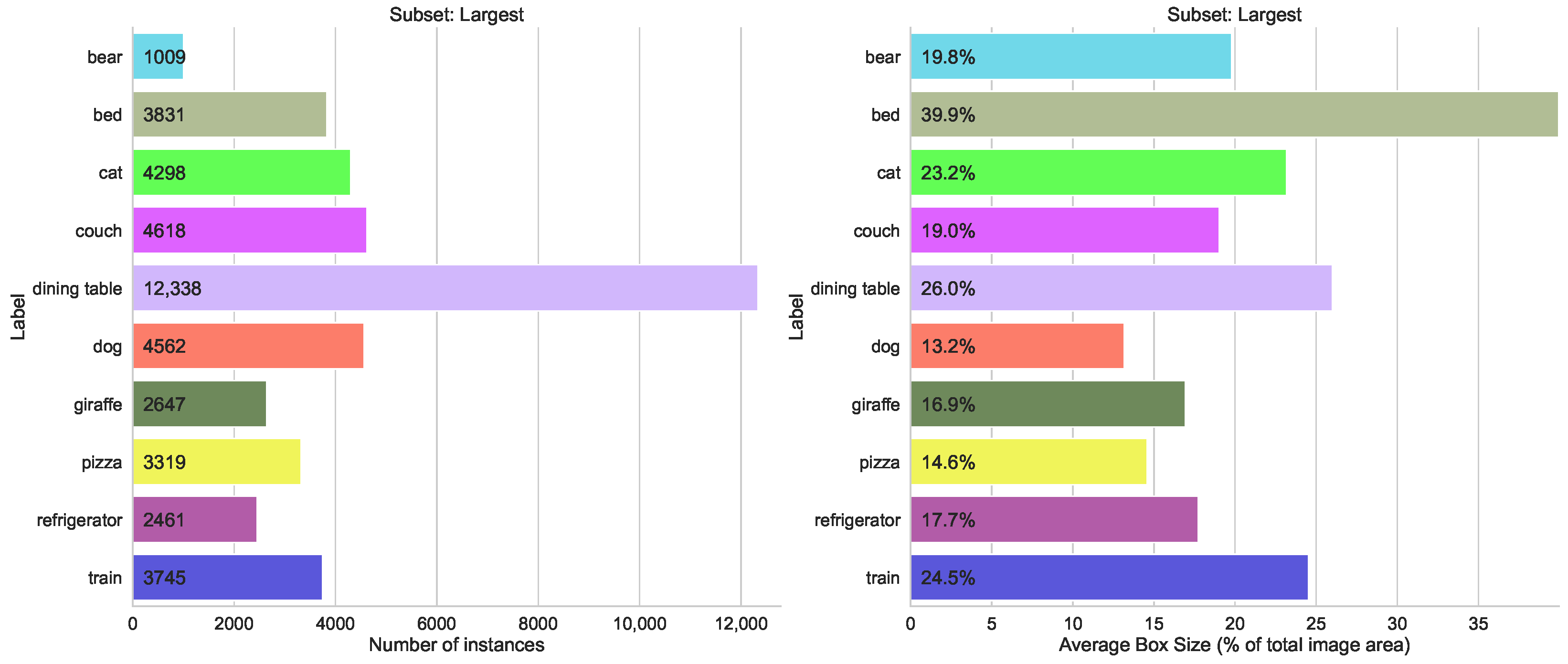
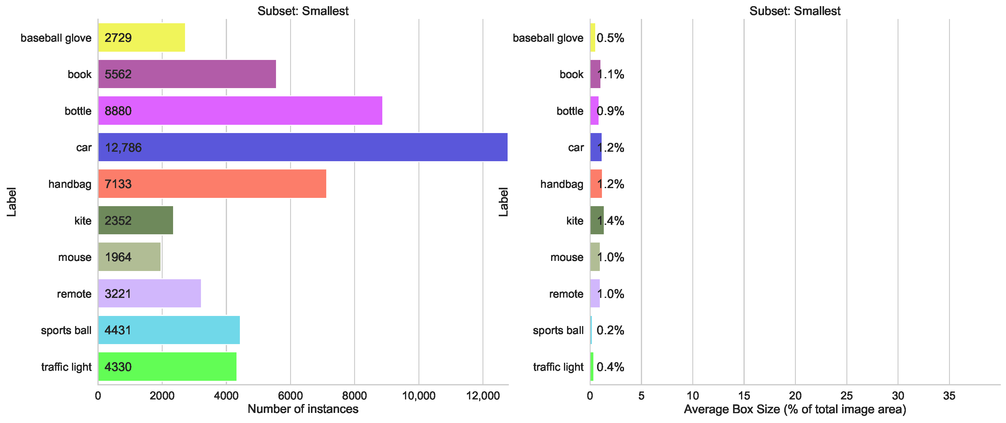
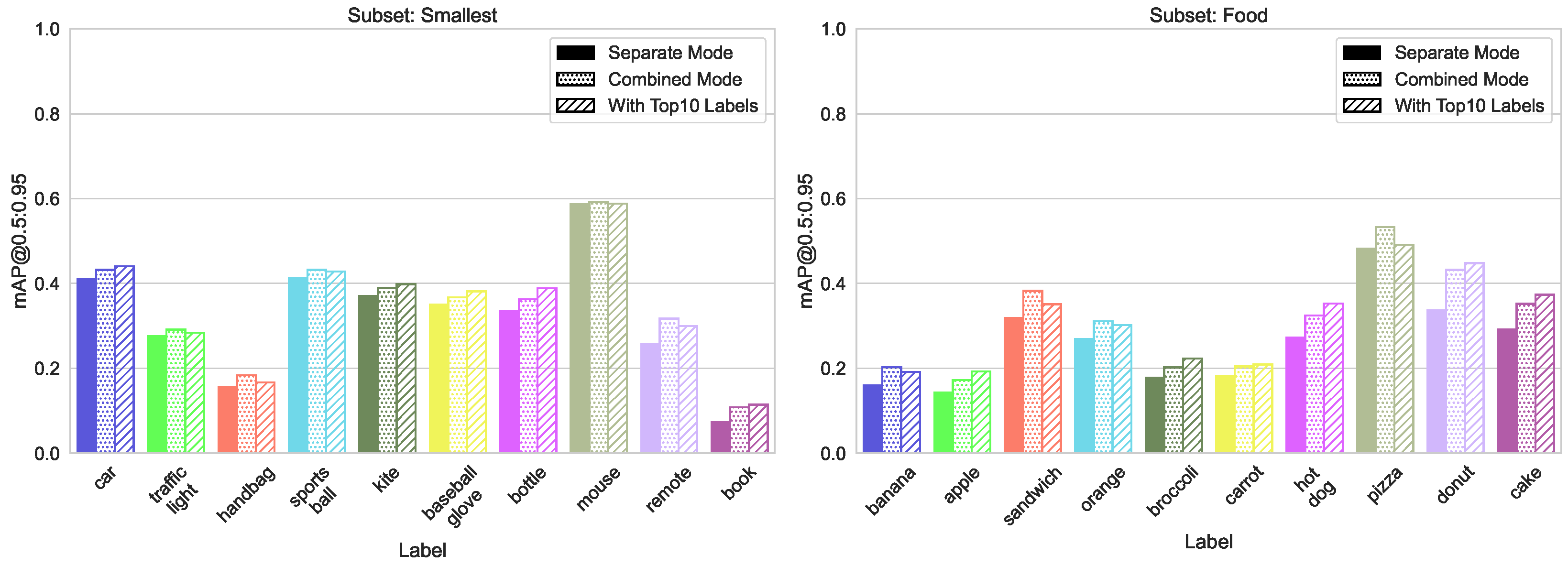
- Box Size split, with two subsets, containing the top 10 classes with the largest average object bounding box sizes, and 10 classes with the lowest average box sizes
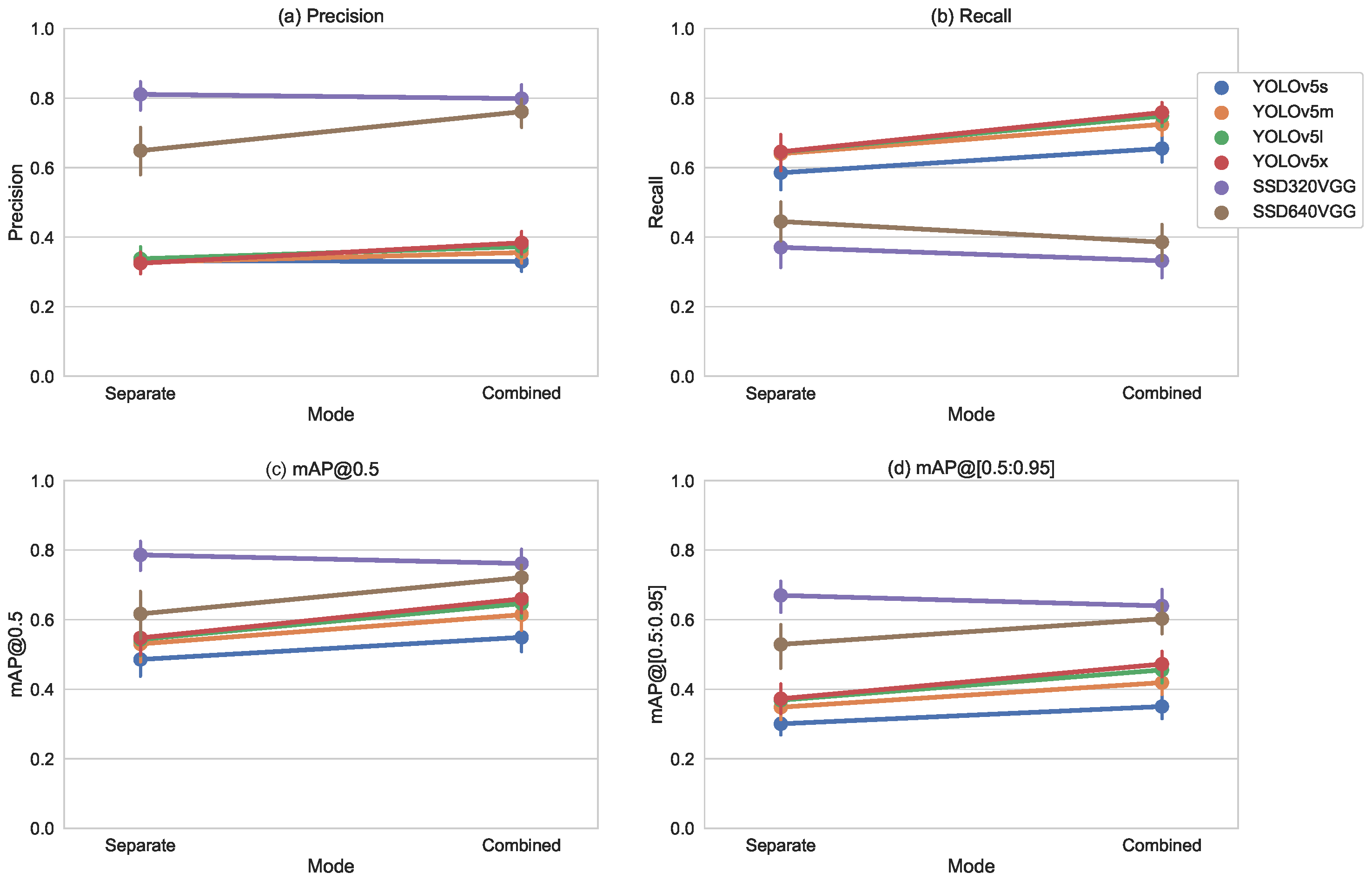
4.2. Models
5. Results
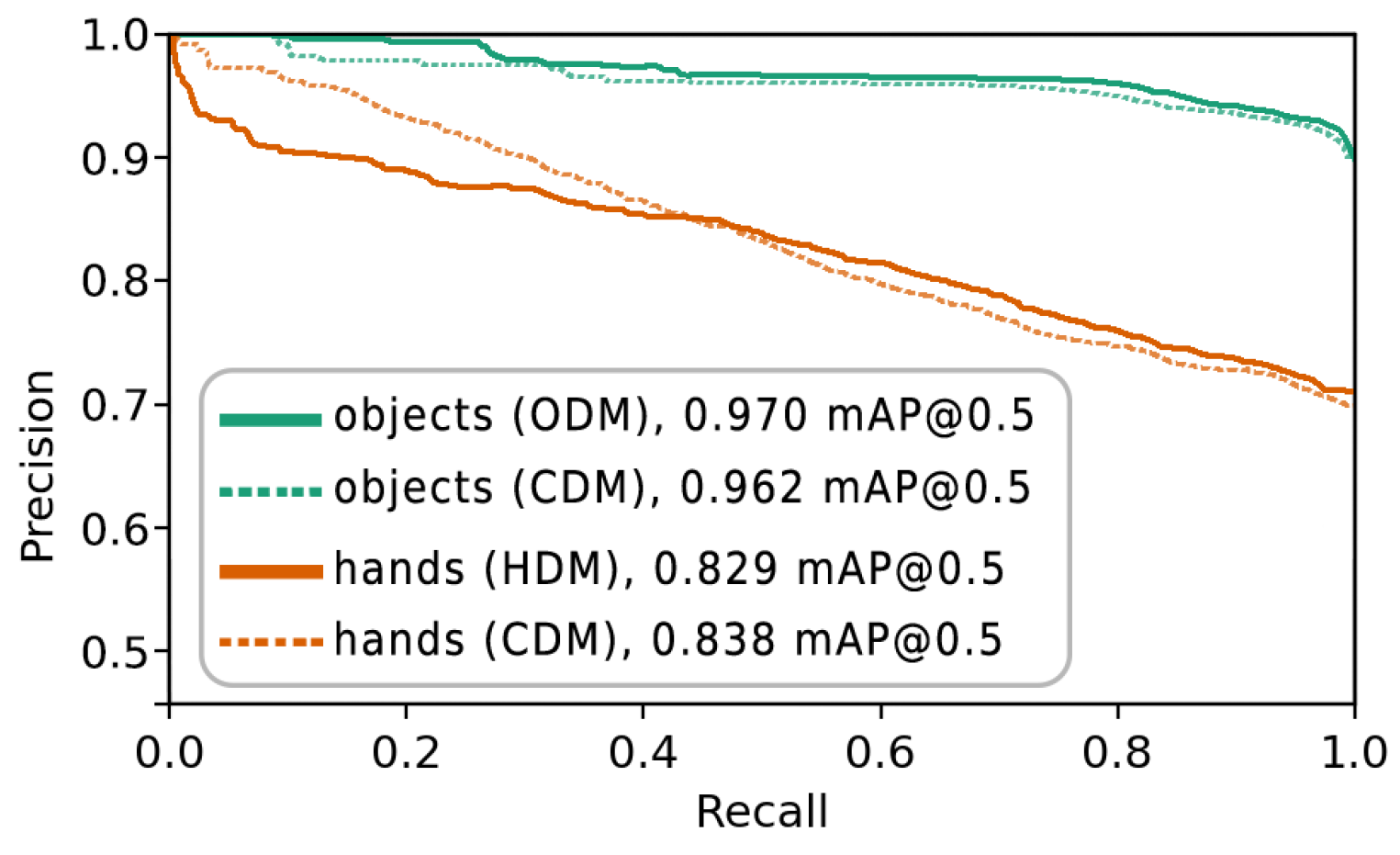
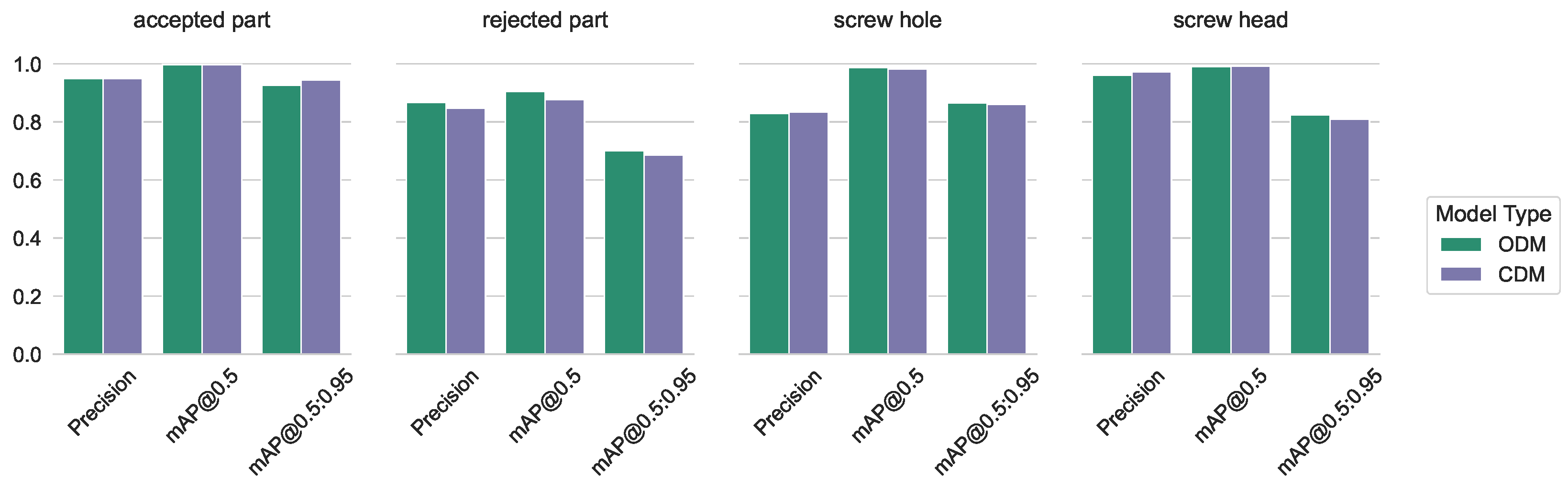
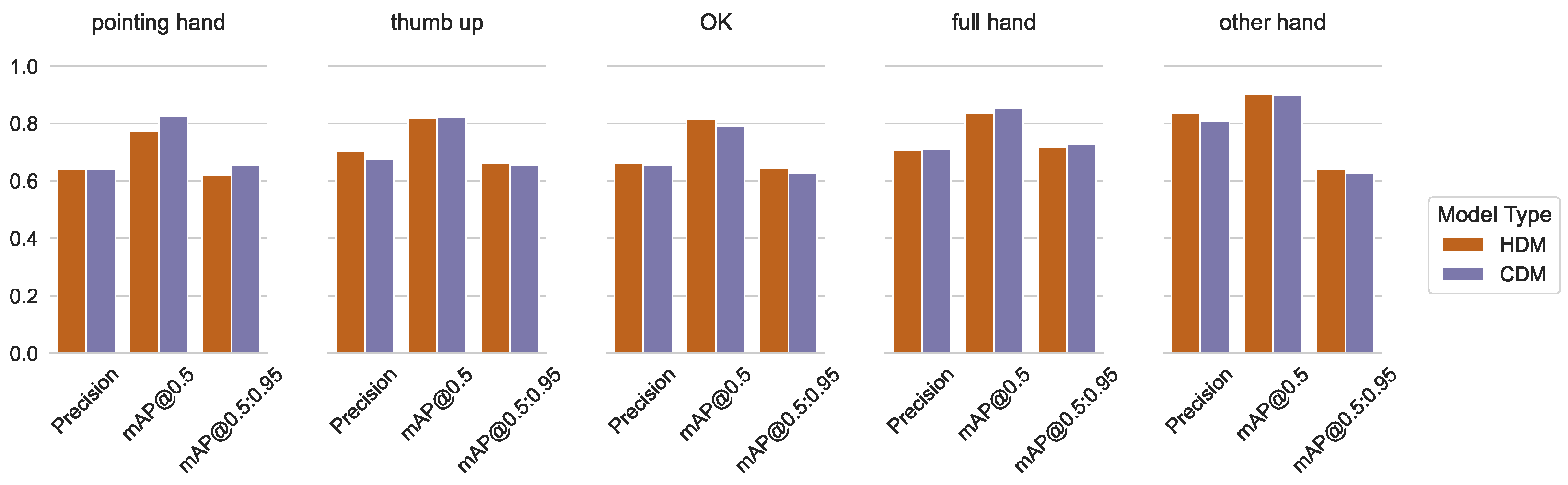
5.1. Accuracy
5.1.1. Our Own Dataset
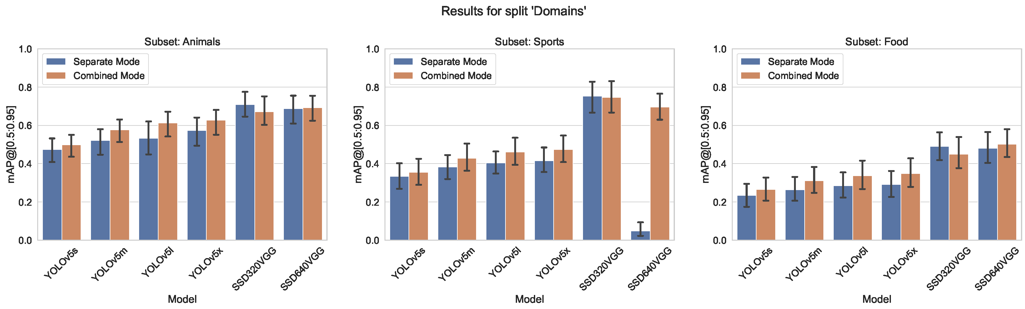
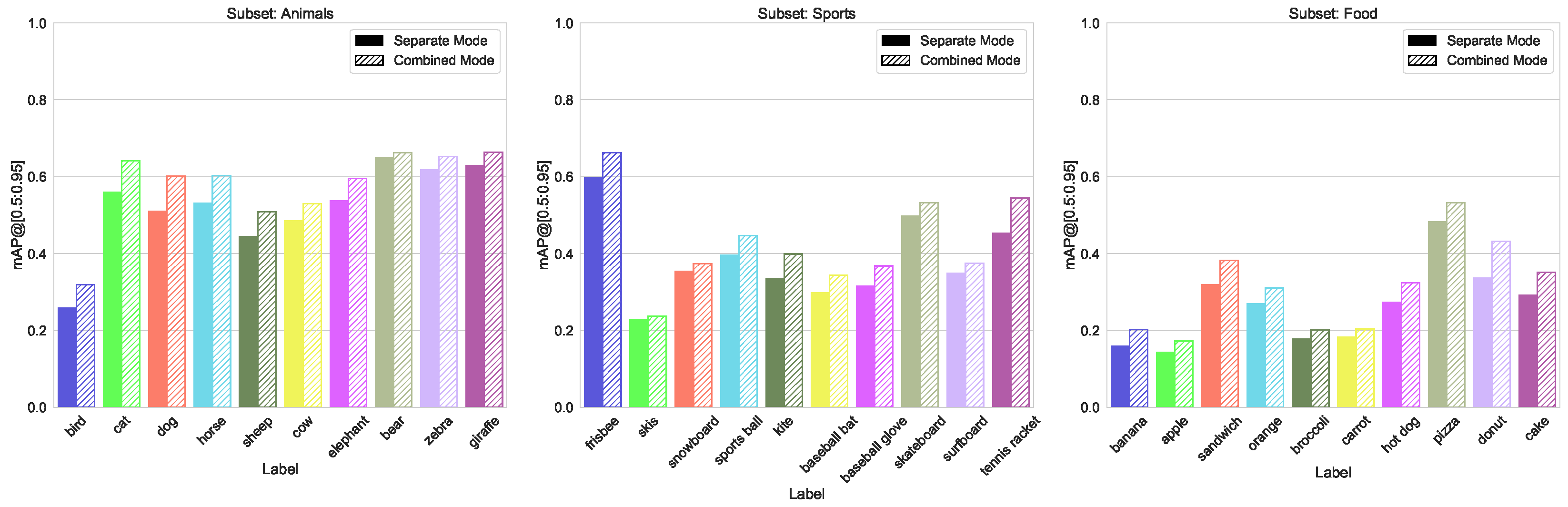
5.1.2. Split by Domain
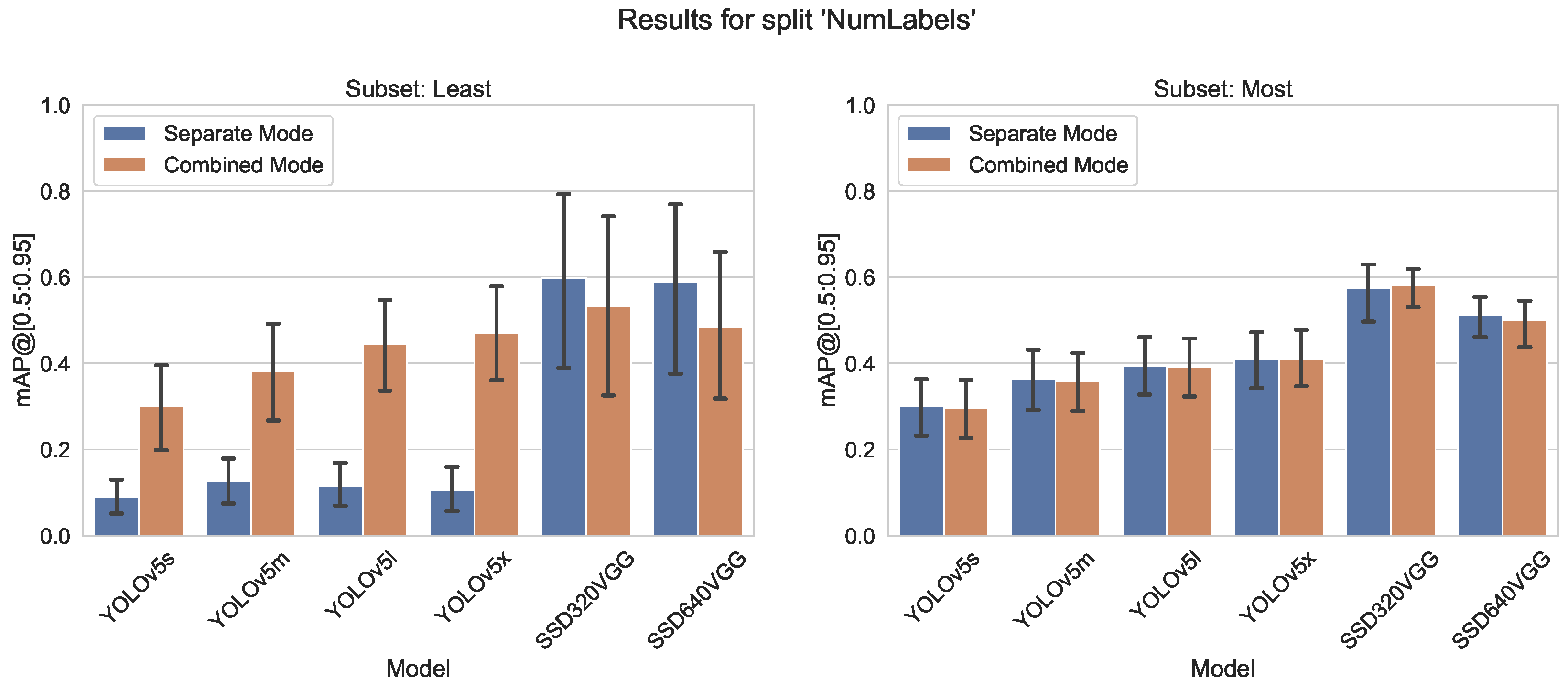
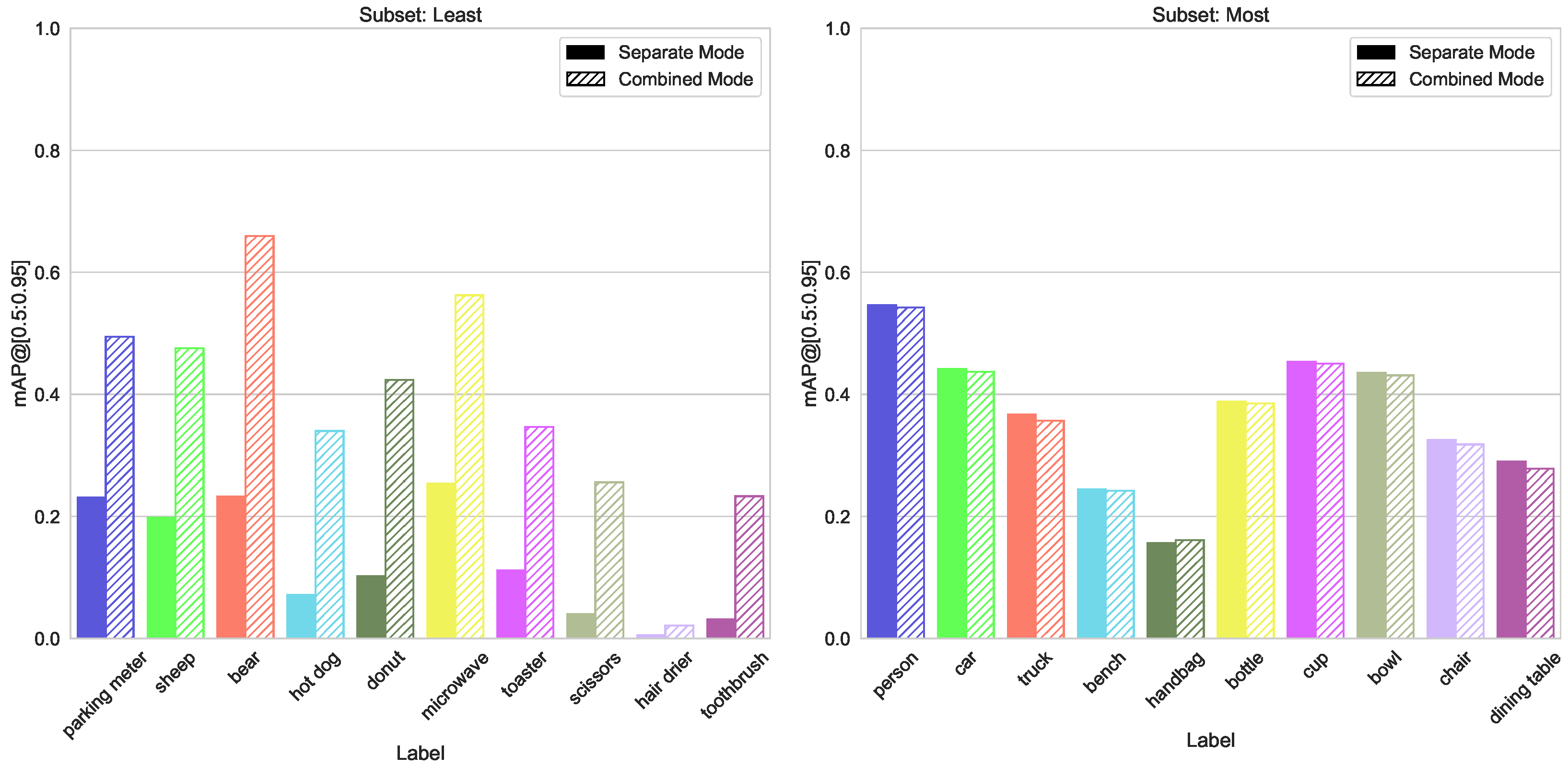
5.1.3. Number of Instances per Label
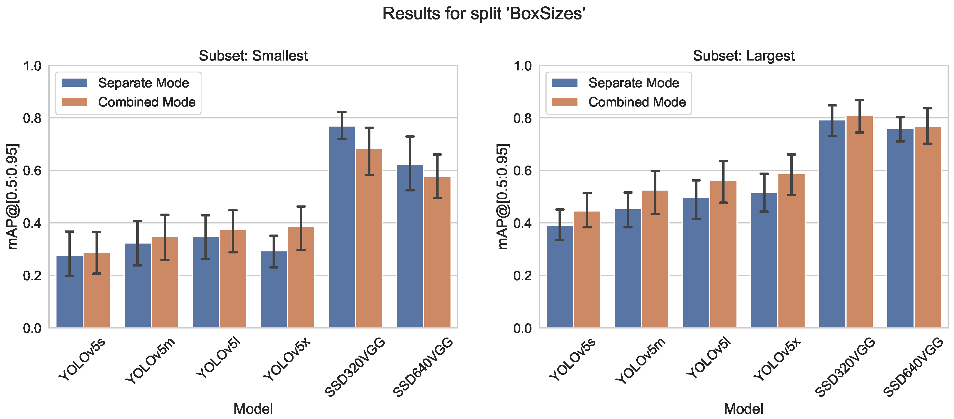
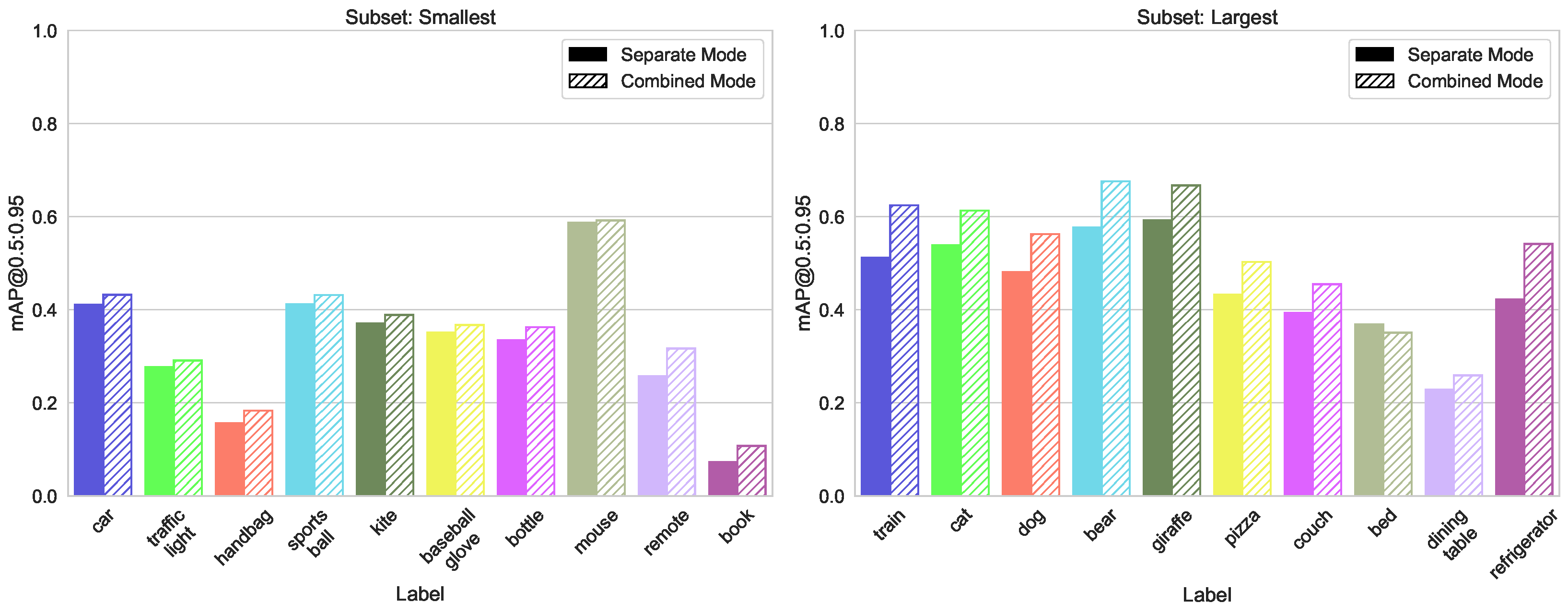
5.1.4. Split by Average Box Size
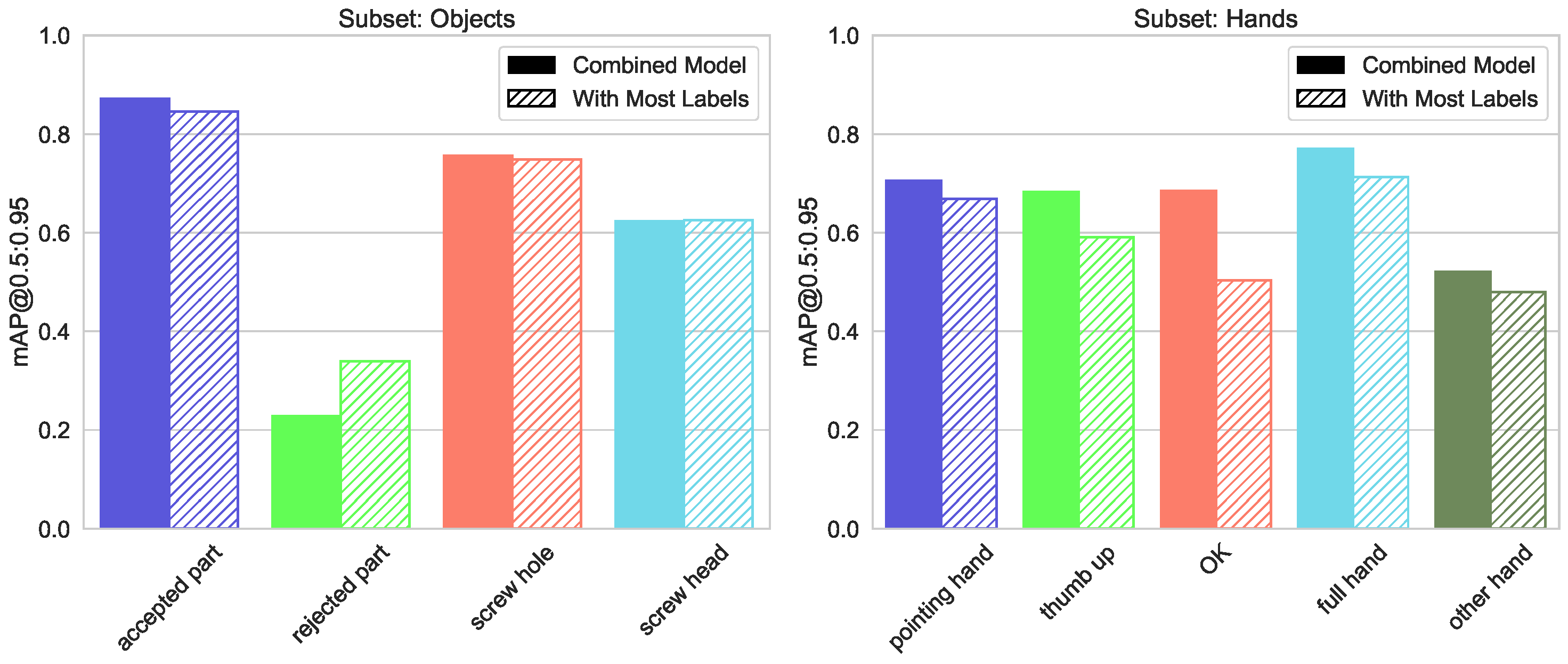
5.1.5. Increase Accuracy by Adding Labels with Many Instances
5.1.6. Overall
5.1.7. Statistics
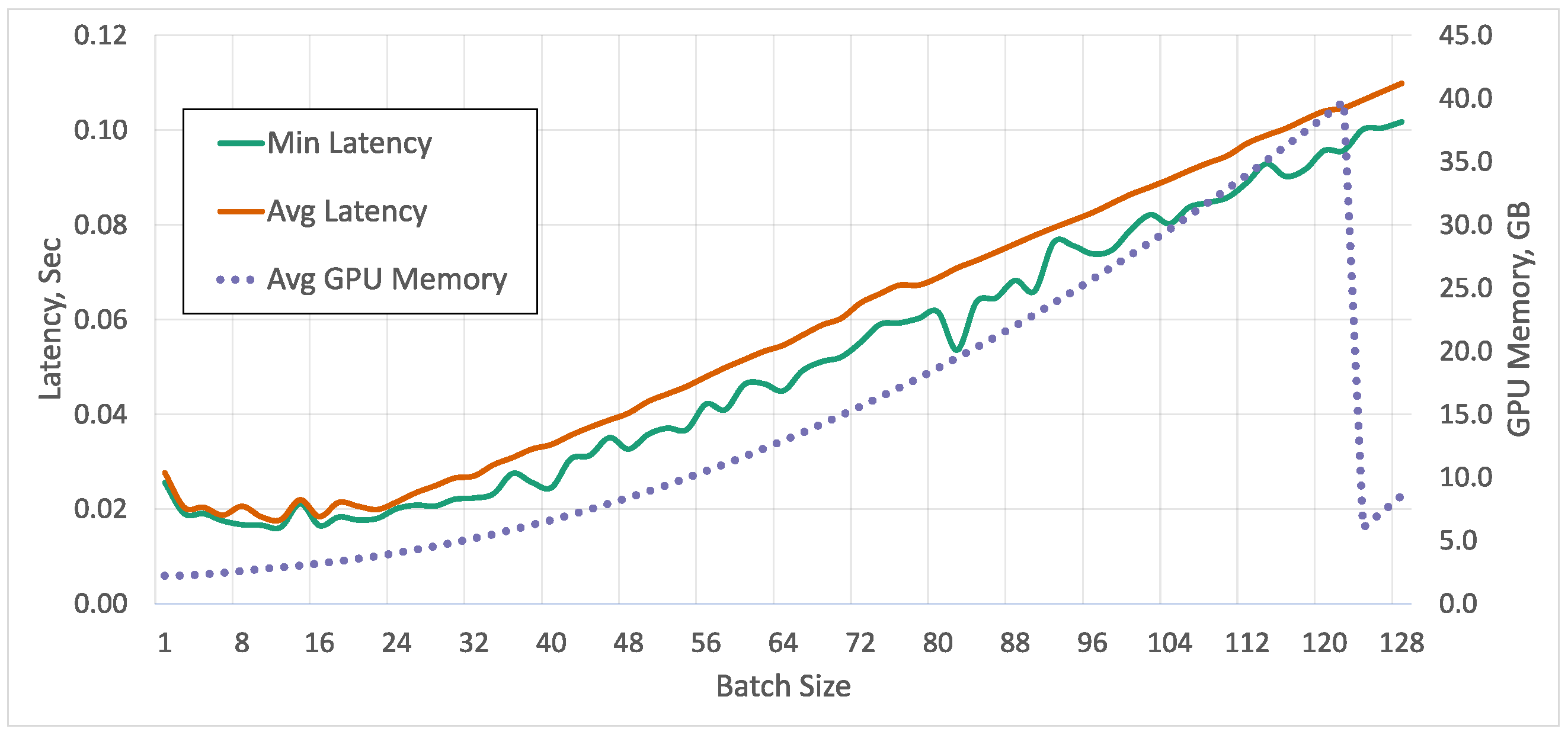
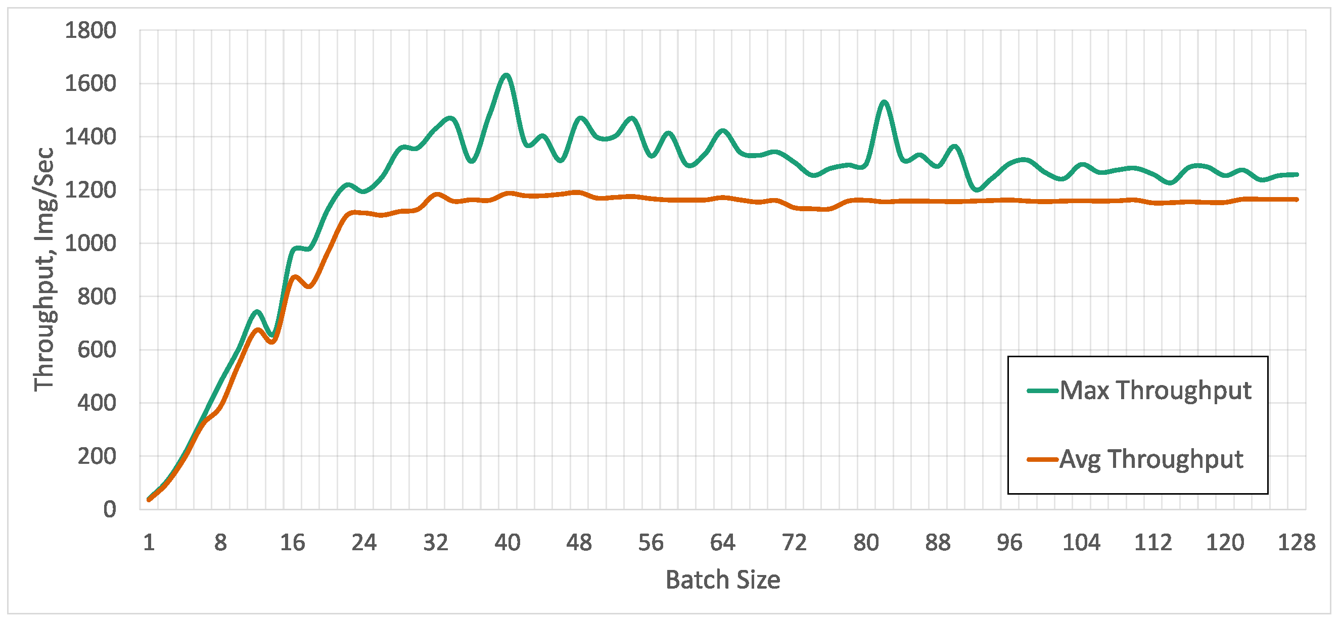
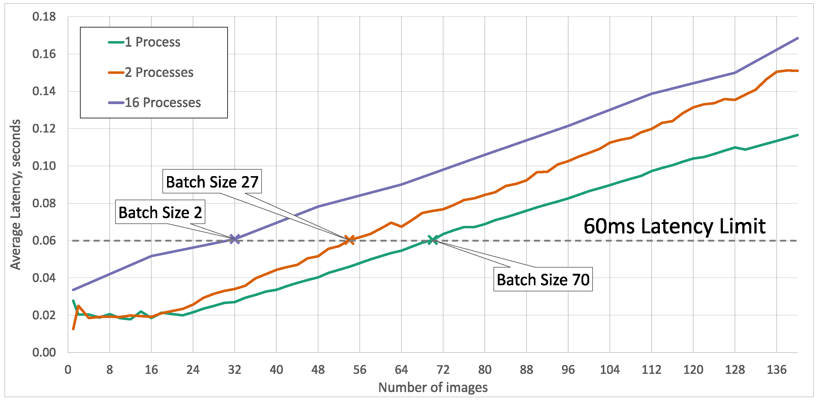
5.2. Processing Time, Memory Consumption
6. Discussion
7. Future Work
8. Conclusions
Author Contributions
Funding
Data Availability Statement
Conflicts of Interest
Abbreviations
| CNN | Convolutional Neural Network |
| COCO | Common Objects in Context |
| ODM | Object-Detection Model |
| HDM | Hand-Detection Model |
| CDM | Combined Detection Model |
| IoU | Intersection over Union |
| mAP@0.5 | Mean Average Precision at IoU threshold of 0.5 |
| mAP@[0.5:0.95] | Mean Average Precision averaged at 10 IoU thresholds in range from 0.5 to 0.95 |
| NMS | Non-Maximum Suppression |
| SSD | Single Shot MultiBox Detector |
| TSN | Time-Sensitive Networking |
| YOLO | You Only Look Once |
| RCNN | Region-based CNN |
References
- Nuzzi, C.; Pasinetti, S.; Lancini, M.; Docchio, F.; Sansoni, G. Deep learning-based hand gesture recognition for collaborative robots. IEEE Instrum. Meas. Mag. 2019, 22, 44–51. [Google Scholar] [CrossRef]
- Newman, T.S.; Jain, A.K. A Survey of Automated Visual Inspection. Comput. Vis. Image Underst. 1995, 61, 231–262. [Google Scholar] [CrossRef]
- Nath, V.; Chattopadhyay, C. S2D2Net: An Improved Approach For Robust Steel Surface Defects Diagnosis with Small Sample Learning. In Proceedings of the 2021 IEEE International Conference on Image Processing (ICIP), Anchorage, AK, USA, 19–22 September 2021; pp. 1199–1203. [Google Scholar] [CrossRef]
- Cambeiro, A.; Seibold, C.; Hilsmann, A.; Eisert, P. Automated Damage Inspection of Power Transmission Towers from UAV Images. In Proceedings of the International Conference on Computer Vision Theory and Applications, Online, 6–8 February 2022; Volume 5, pp. 382–389. [Google Scholar] [CrossRef]
- Ren, Z.; Fang, F.; Yan, N.; Wu, Y. State of the Art in Defect Detection Based on Machine Vision. Int. J. Precis. Eng.-Manuf.-Green Technol. 2022, 9, 661–691. [Google Scholar] [CrossRef]
- Krishna Chand Gudi, S.L.; Ojha, S.; Johnston, B.; Clark, J.; Williams, M.A. Fog Robotics for Efficient, Fluent and Robust Human-Robot Interaction. In Proceedings of the 2018 IEEE 17th International Symposium on Network Computing and Applications (NCA), Cambridge, MA, USA, 1–3 November 2018; pp. 1–5. [Google Scholar] [CrossRef]
- Padmanabhan, A.; Agarwal, N.; Iyer, A.; Ananthanarayanan, G.; Shu, Y.; Karianakis, N.; Xu, G.H.; Netravali, R. Gemel: Model Merging for {Memory-Efficient}, {Real-Time} Video Analytics at the Edge. In Proceedings of the 20th USENIX Symposium on Networked Systems Design and Implementation, Boston, MA, USA, 17–19 April 2023; pp. 973–994. [Google Scholar]
- Jeong, J.S.; Kim, S.; Yu, G.I.; Lee, Y.; Chun, B.G. Accelerating Multi-Model Inference by Merging DNNs of Different Weights. Technical Report. arXiv 2020, arXiv:2009.13062. [Google Scholar] [CrossRef]
- Lin, T.Y.; Maire, M.; Belongie, S.; Hays, J.; Perona, P.; Ramanan, D.; Dollár, P.; Zitnick, C.L. Microsoft coco: Common objects in context. In Proceedings of the Computer Vision–ECCV 2014: 13th European Conference, Zurich, Switzerland, 6–12 September 2014; Proceedings, Part V 13. Springer: Cham, Switzerland, 2014; pp. 740–755. [Google Scholar]
- Afrin, M.; Jin, J.; Rahman, A.; Rahman, A.; Wan, J.; Hossain, E. Resource Allocation and Service Provisioning in Multi-Agent Cloud Robotics: A Comprehensive Survey. IEEE Commun. Surv. Tutor. 2021, 23, 842–870. [Google Scholar] [CrossRef]
- Saeik, F.; Avgeris, M.; Spatharakis, D.; Santi, N.; Dechouniotis, D.; Violos, J.; Leivadeas, A.; Athanasopoulos, N.; Mitton, N.; Papavassiliou, S. Task offloading in Edge and Cloud Computing: A survey on mathematical, artificial intelligence and control theory solutions. Comput. Netw. 2021, 195, 108177. [Google Scholar] [CrossRef]
- Berg, J.; Lu, S. Review of Interfaces for Industrial Human-Robot Interaction. Curr. Robot. Rep. 2020, 1, 27–34. [Google Scholar] [CrossRef]
- Strazdas, D.; Hintz, J.; Felßberg, A.M.; Al-Hamadi, A. Robots and Wizards: An Investigation Into Natural Human–Robot Interaction. IEEE Access 2020, 8, 207635–207642. [Google Scholar] [CrossRef]
- Mohamed, N.; Mustafa, M.B.; Jomhari, N. A Review of the Hand Gesture Recognition System: Current Progress and Future Directions. IEEE Access 2021, 9, 157422–157436. [Google Scholar] [CrossRef]
- Rahman, A.; Kovalenko, M.; Przewozny, D.; Dawoud, K.; Chojecki, P.; Eisert, P.; Bosse, S. Can You Do Real-Time Gesture Recognition with 5 Watts? In Proceedings of the 2021 IEEE International Conference on Systems, Man, and Cybernetics (SMC), Melbourne, Australia, 17–20 October 2021; pp. 2584–2589. [Google Scholar] [CrossRef]
- Jezek, S.; Jonak, M.; Burget, R.; Dvorak, P.; Skotak, M. Deep learning-based defect detection of metal parts: Evaluating current methods in complex conditions. In Proceedings of the 2021 13th International Congress on Ultra Modern Telecommunications and Control Systems and Workshops (ICUMT), Brno, Czech Republic, 25–27 October 2021; pp. 66–71. [Google Scholar] [CrossRef]
- Andrei-Alexandru, T.; Cosmin, C.; Bogdan, P.; Adrian-Alexandru, T. Automated ceramic plate defect detection using ScaledYOLOv4-large. In Proceedings of the 2021 13th International Conference on Electronics, Computers and Artificial Intelligence (ECAI), Pitesti, Romania, 1–3 July 2021; pp. 1–6. [Google Scholar] [CrossRef]
- Aziz, L.; Haji Salam, M.S.B.; Sheikh, U.U.; Ayub, S. Exploring Deep Learning-Based Architecture, Strategies, Applications and Current Trends in Generic Object Detection: A Comprehensive Review. IEEE Access 2020, 8, 170461–170495. [Google Scholar] [CrossRef]
- Lee, J.H.; Kim, B.H.; Kim, M.Y. Machine Learning-based Automatic Optical Inspection System with Multimodal Optical Image Fusion Network. Int. J. Control. Autom. Syst. 2021, 19, 3503–3510. [Google Scholar] [CrossRef]
- Foggia, P.; Greco, A.; Saggese, A.; Vento, M. Multi-task learning on the edge for effective gender, age, ethnicity and emotion recognition. Eng. Appl. Artif. Intell. 2023, 118, 105651. [Google Scholar] [CrossRef]
- Żarski, M.; Wójcik, B.; Książek, K.; Miszczak, J.A. Finicky transfer learning—A method of pruning convolutional neural networks for cracks classification on edge devices. Comput.-Aided Civ. Infrastruct. Eng. 2022, 37, 500–515. [Google Scholar] [CrossRef]
- Pruning/Sparsity Tutorial—Ultralytics YOLOv8 Docs. Available online: https://docs.ultralytics.com/yolov5/tutorials/model_pruning_and_sparsity/#test-normally (accessed on 15 June 2023).
- Rivas, D.; Guim, F.; Polo, J.; Carrera, D. Performance characterization of video analytics workloads in heterogeneous edge infrastructures. Concurr. Comput. Pract. Exp. 2023, 35, e6317. [Google Scholar] [CrossRef]
- Xiao, Z.; Xia, Z.; Zheng, H.; Zhao, B.Y.; Jiang, J. Towards Performance Clarity of Edge Video Analytics. In Proceedings of the 2021 IEEE/ACM Symposium on Edge Computing (SEC), San Jose, CA, USA, 14–17 December 2021; pp. 148–164. [Google Scholar]
- Cozzolino, V.; Tonetto, L.; Mohan, N.; Ding, A.Y.; Ott, J. Nimbus: Towards Latency-Energy Efficient Task Offloading for AR Services. IEEE Trans. Cloud Comput. 2022, 11, 1530–1545. [Google Scholar] [CrossRef]
- Tanwani, A.K.; Anand, R.; Gonzalez, J.E.; Goldberg, K. RILaaS: Robot Inference and Learning as a Service. IEEE Robot. Autom. Lett. 2020, 5, 4423–4430. [Google Scholar] [CrossRef]
- Hanhirova, J.; Kämäräinen, T.; Seppälä, S.; Siekkinen, M.; Hirvisalo, V.; Ylä-Jääski, A. Latency and throughput characterization of convolutional neural networks for mobile computer vision. In Proceedings of the 9th ACM Multimedia Systems Conference, Amsterdam, The Netherlands, 12–15 June 2018; pp. 204–215. [Google Scholar]
- Jahanshahi, A.; Sabzi, H.Z.; Lau, C.; Wong, D. GPU-NEST: Characterizing Energy Efficiency of Multi-GPU Inference Servers. IEEE Comput. Archit. Lett. 2020, 19, 139–142. [Google Scholar] [CrossRef]
- Jain, P.; Mo, X.; Jain, A.; Subbaraj, H.; Durrani, R.S.; Tumanov, A.; Gonzalez, J.; Stoica, I. Dynamic space-time scheduling for gpu inference. arXiv 2018, arXiv:1901.00041. [Google Scholar]
- Srivastava, A.; Nguyen, D.; Aggarwal, S.; Luckow, A.; Duffy, E.; Kennedy, K.; Ziolkowski, M.; Apon, A. Performance and memory trade-offs of deep learning object detection in fast streaming high-definition images. In Proceedings of the 2018 IEEE International Conference on Big Data (Big Data), Seattle, WA, USA, 10–13 December 2018; pp. 3915–3924. [Google Scholar]
- Fang, J.; Liu, Q.; Li, J. A Deployment Scheme of YOLOv5 with Inference Optimizations Based on the Triton Inference Server. In Proceedings of the 2021 IEEE 6th International Conference on Cloud Computing and Big Data Analytics (ICCCBDA), Chengdu, China, 24–26 April 2021; pp. 441–445. [Google Scholar] [CrossRef]
- Padmanabhan, A.; Iyer, A.P.; Ananthanarayanan, G.; Shu, Y.; Karianakis, N.; Xu, G.H.; Netravali, R. Towards memory-efficient inference in edge video analytics. In Proceedings of the 3rd ACM Workshop on Hot Topics in Video Analytics and Intelligent Edges, New Orleans, LA, USA, 25 October 2021; pp. 31–37. [Google Scholar]
- Lee, J.; Liu, Y.; Lee, Y. ParallelFusion: Towards Maximum Utilization of Mobile GPU for DNN Inference. In Proceedings of the 5th International Workshop on Embedded and Mobile Deep Learning, EMDL’21, Virtual, 24–25 June 2021; Association for Computing Machinery: New York, NY, USA, 2021; pp. 25–30. [Google Scholar] [CrossRef]
- Rivas, D.; Guim, F.; Polo, J.; Silva, P.M.; Berral, J.L.; Carrera, D. Towards automatic model specialization for edge video analytics. Future Gener. Comput. Syst. 2022, 134, 399–413. [Google Scholar] [CrossRef]
- Kim, D.; Lee, S.; Sung, N.M.; Choe, C. Real-time object detection using a domain-based transfer learning method for resource-constrained edge devices. In Proceedings of the 2023 International Conference on Artificial Intelligence in Information and Communication (ICAIIC), Bali, Indonesia, 20–23 February 2023; pp. 457–462, ISSN 2831-6983. [Google Scholar] [CrossRef]
- Wang, C.Y.; Bochkovskiy, A.; Liao, H.Y.M. YOLOv7: Trainable bag-of-freebies sets new state-of-the-art for real-time object detectors. In Proceedings of the IEEE/CVF Conference on Computer Vision and Pattern Recognition, Vancouver, BC, Canada, 18–22 June 2023; pp. 7464–7475. [Google Scholar]
- Stone, T.; Stone, N.; Jain, P.; Jiang, Y.; Kim, K.H.; Nelakuditi, S. Towards Scalable Video Analytics at the Edge. In Proceedings of the 2019 16th Annual IEEE International Conference on Sensing, Communication, and Networking (SECON), Boston, MA, USA, 10–13 June 2019; pp. 1–9, ISSN 2155-5494. [Google Scholar] [CrossRef]
- Hu, X.; Chu, L.; Pei, J.; Liu, W.; Bian, J. Model complexity of deep learning: A survey. Knowl. Inf. Syst. 2021, 63, 2585–2619. [Google Scholar] [CrossRef]
- Popper, J.; Harms, C.; Ruskowski, M. Enabling reliable visual quality control in smart factories through TSN. Procedia CIRP 2020, 88, 549–553. [Google Scholar] [CrossRef]
- Vick, A.; Krueger, J. Using OPC UA for distributed industrial robot control. In Proceedings of the ISR 2018; 50th International Symposium on Robotics, Munich, Germany, 20–21 June 2018; VDE: Offenbach am Main, Germany; pp. 1–6. [Google Scholar]
- Liu, W.; Anguelov, D.; Erhan, D.; Szegedy, C.; Reed, S.; Fu, C.Y.; Berg, A.C. Ssd: Single shot multibox detector. In Proceedings of the Computer Vision–ECCV 2016: 14th European Conference, Amsterdam, The Netherlands, 11–14 October 2016; Proceedings, Part I 14. Springer International Publishing: Cham, Switzerland, 2016; pp. 21–37. [Google Scholar]
- Jocher, G.; Stoken, A.; Chaurasia, A.; Borovec, J.; NanoCode012; TaoXie; Kwon, Y.; Michael, K.; Changyu, L.; Fang, J.; et al. Ultralytics/yolov5: V6.0—YOLOv5n ’Nano’ Models, Roboflow Integration, TensorFlow Export, OpenCV DNN Support. 2021; Available online: https://doi.org/10.5281/zenodo.5563715 (accessed on 2 February 2022).
- Ren, S.; He, K.; Girshick, R.; Sun, J. Faster r-cnn: Towards real-time object detection with region proposal networks. Adv. Neural Inf. Process. Syst. 2015, 28, 91–99. [Google Scholar] [CrossRef] [PubMed]
- Zhao, S.; Zheng, J.; Sun, S.; Zhang, L. An Improved YOLO Algorithm for Fast and Accurate Underwater Object Detection. Symmetry 2022, 14, 1669. [Google Scholar] [CrossRef]
- Padilla, R.; Netto, S.L.; da Silva, E.A.B. A Survey on Performance Metrics for Object-Detection Algorithms. In Proceedings of the 2020 International Conference on Systems, Signals and Image Processing (IWSSIP), Niteroi, Brazil, 1–3 July 2020; pp. 237–242. [Google Scholar] [CrossRef]
- Padilla, R.; Passos, W.L.; Dias, T.L.; Netto, S.L.; Da Silva, E.A. A comparative analysis of object detection metrics with a companion open-source toolkit. Electronics 2021, 10, 279. [Google Scholar] [CrossRef]
- Liu, G.; Nouaze, J.C.; Touko Mbouembe, P.L.; Kim, J.H. YOLO-tomato: A robust algorithm for tomato detection based on YOLOv3. Sensors 2020, 20, 2145. [Google Scholar] [CrossRef] [PubMed]
- Wilcoxon, F. Individual Comparisons by Ranking Methods. In Breakthroughs in Statistics: Methodology and Distribution; Kotz, S., Johnson, N.L., Eds.; Springer Series in Statistics; Springer: New York, NY, USA, 1992; pp. 196–202. [Google Scholar] [CrossRef]
- Vallat, R. Pingouin: Statistics in Python. J. Open Source Softw. 2018, 3, 1026. [Google Scholar] [CrossRef]
- Tips for Best Training Results · Ultralytics/yolov5 Wiki · GitHub. Available online: https://github.com/ultralytics/yolov5/wiki/Tips-for-Best-Training-Results (accessed on 2 October 2022).
- Xia, X.; Meng, Z.; Han, X.; Li, H.; Tsukiji, T.; Xu, R.; Zheng, Z.; Ma, J. An automated driving systems data acquisition and analytics platform. Transp. Res. Part C Emerg. Technol. 2023, 151, 104120. [Google Scholar] [CrossRef]
- Kuznetsova, A.; Rom, H.; Alldrin, N.; Uijlings, J.; Krasin, I.; Pont-Tuset, J.; Kamali, S.; Popov, S.; Malloci, M.; Kolesnikov, A.; et al. The open images dataset v4: Unified image classification, object detection, and visual relationship detection at scale. Int. J. Comput. Vis. 2020, 128, 1956–1981. [Google Scholar] [CrossRef]
- McMahan, B.; Moore, E.; Ramage, D.; Hampson, S.; y Arcas, B.A. Communication-efficient learning of deep networks from decentralized data. In Proceedings of the Artificial Intelligence and Statistics, PMLR, Fort Lauderdale, FL, USA, 20–22 April 2017; pp. 1273–1282. [Google Scholar]


| Model | Size | Latency | mAP@[0.5:0.95] |
|---|---|---|---|
| YOLOv5s | 14.3 MB | 19.82 ms | 0.638 |
| YOLOv5m | 42.2 MB | 25.00 ms | 0.649 |
| YOLOv5l | 92.9 MB | 32.87 ms | 0.672 |
| YOLOv5x | 173.2 MB | 38.77 ms | 0.659 |
| SSD320 | 96.9 MB | 23.58 ms | 0.114 |
| SSD640 | 96.9 MB | 23.73 ms | 0.233 |
| Faster-RCNN | 162.0 MB | 59.69 ms | 0.460 |
| Running Model(-s) | Average Latency, ms | Waiting for Next Frame, ms | |
|---|---|---|---|
| HDM only | |||
| ODM only | |||
| Concurrently | HDM | ||
| ODM | |||
| CDM | |||
| GPU | Latency, ms | ||
|---|---|---|---|
| Min | Mean | Max | |
| RTX 3080 | 20.6 | 25.7 | 39.8 |
| A100 | 25.4 | 30.1 | 39.6 |
| RTX 2080 Ti | 35.7 | 40.4 | 55.1 |
| Concurrent Images (Processes × Batch Size) | Average Latency, ms | |
|---|---|---|
| CUDA 10.2 | CUDA 11.1 | |
| 1 (1 × 1) | 12.7 | 19.1 |
| 10 (1 × 10) | 33.4 | 36.1 |
| 10 (10 × 1) | 59.2 | 57.1 |
| 16 (1 × 16) | 50.5 | 56.6 |
| 16 (2 × 8) | 50.3 | 53.2 |
| 16 (4 × 4) | 50.2 | 54.4 |
| 16 (8 × 2) | 61.5 | 60.2 |
| 16 (16 × 1) | 93.4 | - |
| 19 (19 × 1) | 59.4 | 65.3 |
Disclaimer/Publisher’s Note: The statements, opinions and data contained in all publications are solely those of the individual author(s) and contributor(s) and not of MDPI and/or the editor(s). MDPI and/or the editor(s) disclaim responsibility for any injury to people or property resulting from any ideas, methods, instructions or products referred to in the content. |
© 2023 by the authors. Licensee MDPI, Basel, Switzerland. This article is an open access article distributed under the terms and conditions of the Creative Commons Attribution (CC BY) license (https://creativecommons.org/licenses/by/4.0/).
Share and Cite
Kovalenko, M.; Przewozny, D.; Eisert, P.; Bosse, S.; Chojecki, P. Data Fusion for Cross-Domain Real-Time Object Detection on the Edge. Sensors 2023, 23, 6138. https://doi.org/10.3390/s23136138
Kovalenko M, Przewozny D, Eisert P, Bosse S, Chojecki P. Data Fusion for Cross-Domain Real-Time Object Detection on the Edge. Sensors. 2023; 23(13):6138. https://doi.org/10.3390/s23136138
Chicago/Turabian StyleKovalenko, Mykyta, David Przewozny, Peter Eisert, Sebastian Bosse, and Paul Chojecki. 2023. "Data Fusion for Cross-Domain Real-Time Object Detection on the Edge" Sensors 23, no. 13: 6138. https://doi.org/10.3390/s23136138
APA StyleKovalenko, M., Przewozny, D., Eisert, P., Bosse, S., & Chojecki, P. (2023). Data Fusion for Cross-Domain Real-Time Object Detection on the Edge. Sensors, 23(13), 6138. https://doi.org/10.3390/s23136138