
LSTMAtU-Net: A Precipitation Nowcasting Model Based on ECSA Module


Abstract
1. Introduction
- 1.
- The LSTMAtU-Net model combines the advantages of RNNs and CNNs. We propose a model that combines the RNN and CNN structures, namely the LSTMAtU-Net model. It has a strong feature extraction capability and improved long-term dependency capabilities, and the core convolutional structure greatly reduces the risk of gradient explosion.
- 2.
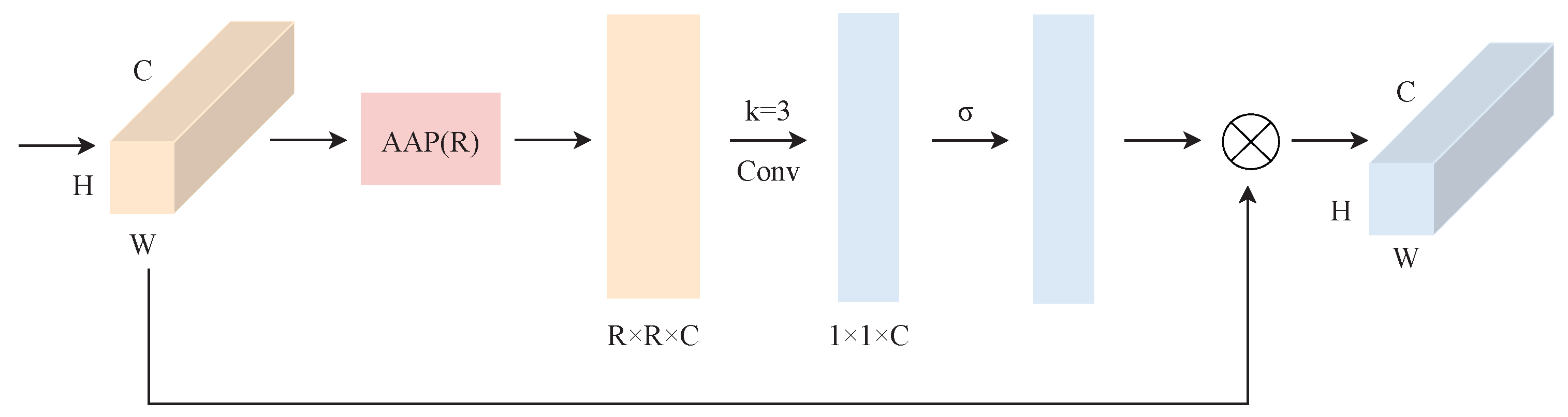
- A new component, the ECSA module, is proposed, which uses mean pooling at different scales as a way to achieve the weighting of the channel and spatial information of convolutional features based on the ECA module [23]; thus, focusing on image details alleviates, to a certain extent, the problem of the RNN’s and CNN’s predictions showing the gradual inaccuracy of the image details.
- 3.
- We propose a completely new loss function. It first optimizes multiple prediction objectives and then designs the corresponding weighted loss function to solve the serious imbalance of precipitation data.
2. Related Works
2.1. Nowcasting Models Based on ConvRNN
2.2. Nowcasting Models Based on U-Net
2.3. Attention Mechanism
3. Methodology
3.1. Problem Definition
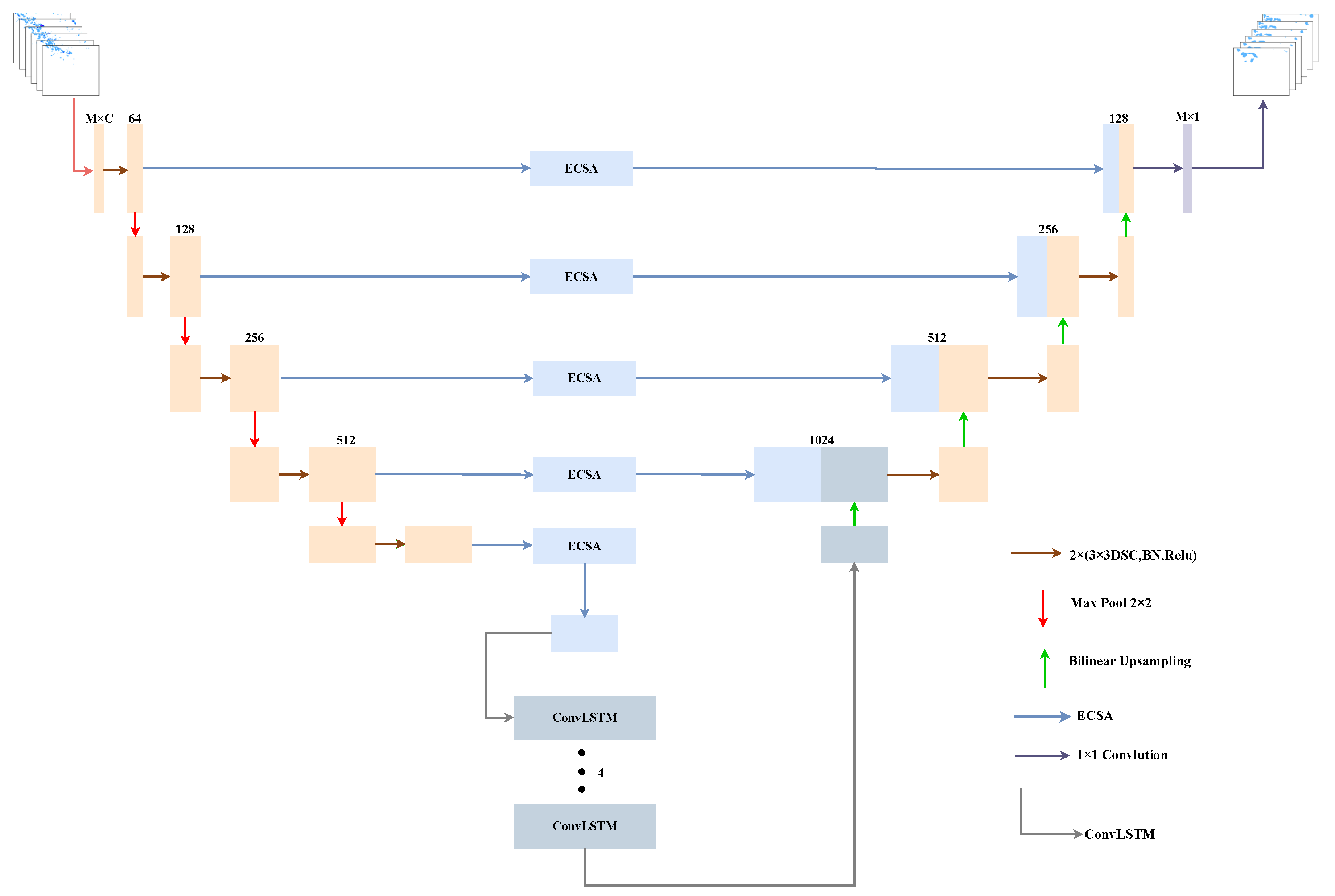
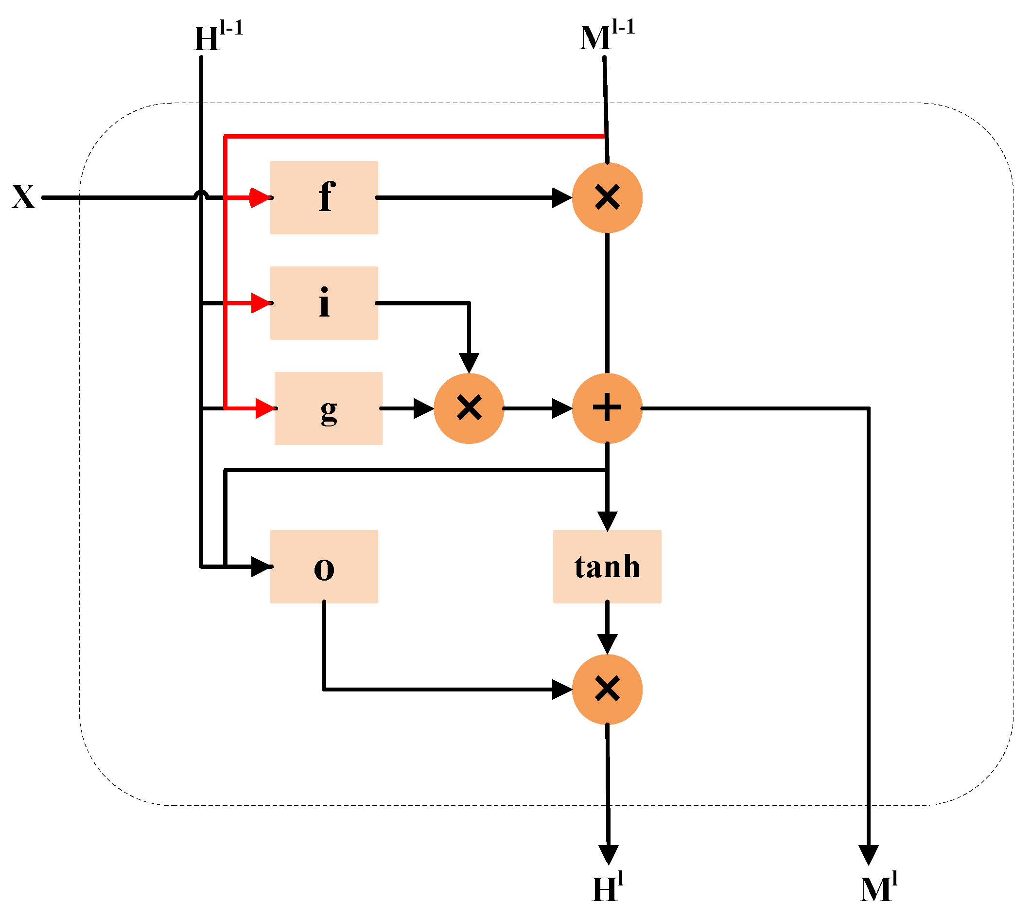
3.2. LSTMAtU-Net
3.3. Loss Function
4. Experiments
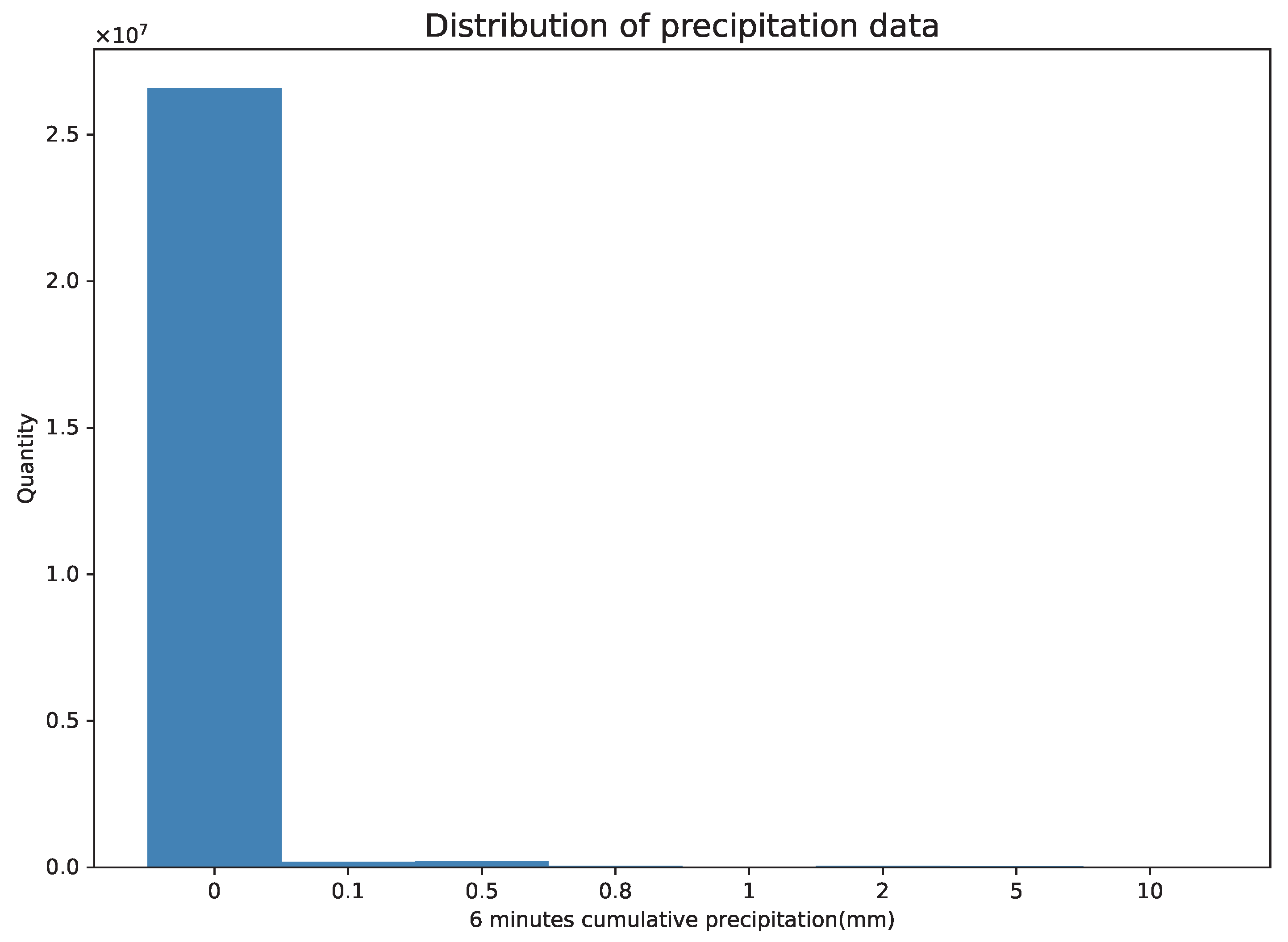
4.1. Dataset
4.2. Performance Metrics
4.3. Implementation Details
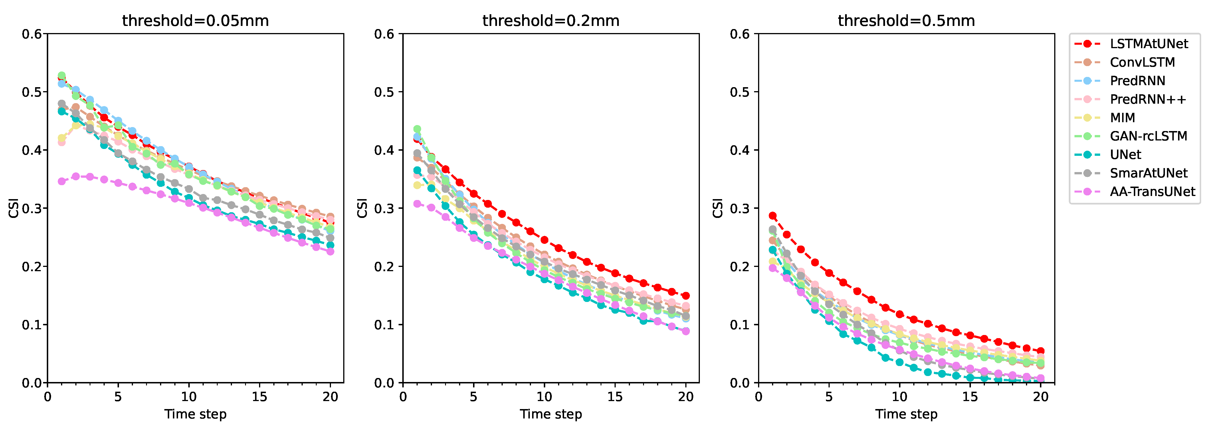
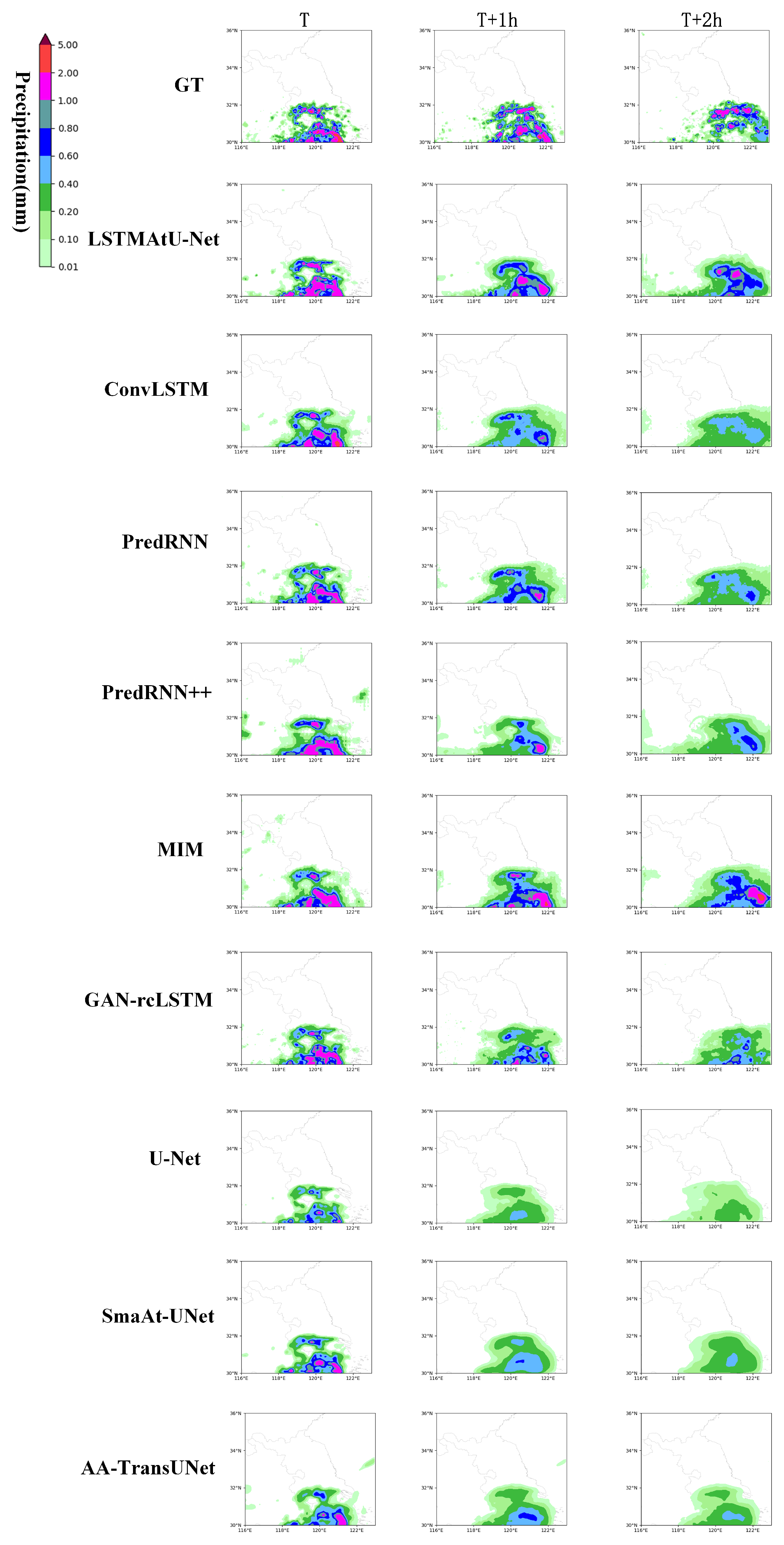
4.4. Quantitative Analysis on the 2022 Jiangsu Weather AI Algorithm Challenge Dataset
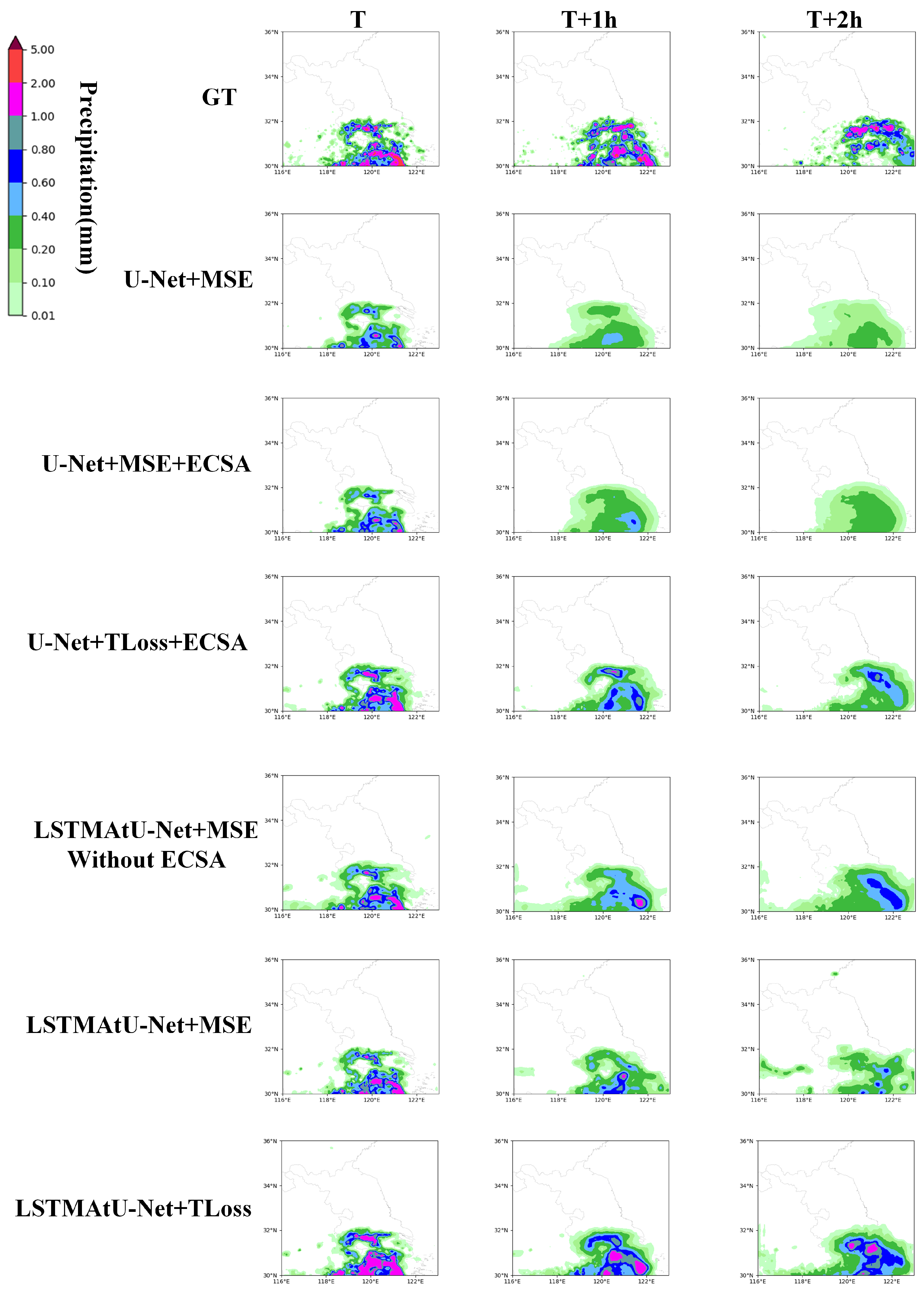
4.5. Ablation Experiments and Analyses
5. Conclusions
Author Contributions
Funding
Institutional Review Board Statement
Informed Consent Statement
Data Availability Statement
Conflicts of Interest
References
- Zhou, J.; Xiang, J.; Huang, S. Classification and Prediction of Typhoon Levels by Satellite Cloud Pictures through GC–LSTM Deep Learning Model. Sensors 2020, 20, 5132. [Google Scholar] [CrossRef] [PubMed]
- Osanai, N.; Shimizu, T.; Kuramoto, K.; Kojima, S.; Noro, T. Japanese early-warning for debris flflows and slope failures using rainfall indices with Radial Basis Function Network. Landslides 2008, 10, 325–338. [Google Scholar]
- Sun, J.; Xue, M.; Wilson, J.W.; Zawadzki, I.; Ballard, S.P.; Onvlee-Hooimeyer, J.; Joe, P.; Barker, D.M.; Li, P.W.; Golding, B.; et al. Use of NWP for nowcasting convective precipitation: Recent progress and challenges. Bull. Am. Meteorol. Soc. 2014, 95, 409–426. [Google Scholar] [CrossRef]
- Chu, Q.; Xu, Z.; Chen, Y.; Han, D. Evaluation of the ability of the Weather Research and Forecasting model to reproduce a sub-daily extreme rainfall event in Beijing, China using different domain confifigurations and spin-up times. Hydrol. Earth Syst. Sci. 2018, 22, 3391–3407. [Google Scholar] [CrossRef]
- Ligda, M. Lightning Detection by Radar. J. Atmos. Terr. Phys. 1956, 9, 279–283. [Google Scholar] [CrossRef]
- Woo, W.C.; Wong, W.K. Operational Application of Optical Flow Techniques to Radar-Based Rainfall Nowcasting. Atmosphere 2017, 8, 48. [Google Scholar] [CrossRef]
- Sakaino, H. Spatio-temporal image pattern prediction method based on a physical model with time-varying optical flow. IEEE Trans. Geosci. Remote Sens. 2013, 51, 3023–3036. [Google Scholar] [CrossRef]
- Germann, U.; Zawadzki, I. Scale-dependence of the predictability of precipitation from continental radar images Part I: Description of the methodology. Mon. Weather. Rev. 2002, 130, 2859–2873. [Google Scholar] [CrossRef]
- Luo, C.; Li, X.; Ye, Y. PFST-LSTM: A SpatioTemporal LSTM Model with Pseudoflflow Prediction for Precipitation Nowcasting. IEEE J. Sel. Top. Appl. Earth Obs. Remote Sens. 2020, 14, 843–857. [Google Scholar] [CrossRef]
- Shi, X.; Chen, Z.; Wang, H.; Yeung, D.Y.; Wong, W.K.; Woo, W.C. Convolutional LSTM Network: A Machine Learning Approach for Precipitation Nowcasting. arXiv 2015, arXiv:1506.04214. [Google Scholar]
- Geng, H.; Wang, T.; Zhuang, X.; Xi, D.; Hu, Z.; Geng, L. GAN-rcLSTM: A Deep Learning Model for Radar Echo Extrapolation. Atmosphere 2022, 13, 684. [Google Scholar] [CrossRef]
- Bowler, N.; Pierce, C.E.; Seed, A. Development of a precipitation nowcasting algorithm based upon optical flow techniques. J. Hydrol. 2004, 288, 74–91. [Google Scholar] [CrossRef]
- Zhang, F.; Wang, X.; Guan, J. A Novel Multi-Input Multi-Output Recurrent Neural Network Based on Multimodal Fusion and Spatiotemporal Prediction for 0–4 Hour Precipitation Nowcasting. Atmosphere 2021, 12, 1596. [Google Scholar] [CrossRef]
- Zhang, F.; Wang, X.; Guan, J.; Wu, M.; Guo, L. RN-Net: A Deep Learning Approach to 0–2 h Rainfall Nowcasting Based on Radar and Automatic Weather Station Data. Sensors 2021, 21, 1981. [Google Scholar] [CrossRef]
- Trebing, K.; Sta`nczyk, T.; Mehrkanoon, S. SmaAt-U-Net: Precipitation nowcasting using a small attention-U-Net architecture. Pattern Recognit. Lett. 2021, 145, 178–186. [Google Scholar] [CrossRef]
- Yang, Y.; Mehrkanoon, S. Aa-transunet: Attention augmented transunet for nowcasting tasks. In Proceedings of the 2022 International Joint Conference on Neural Networks (IJCNN), Padua, Italy, 18–23 July 2022. [Google Scholar]
- Bouget, V.; Béréziat, D.; Brajard, J.; Charantonis, A.; Filoche, A. Fusion of Rain Radar Images and Wind Forecasts in a Deep Learning Model Applied to Rain Nowcasting. Remote Sens. 2021, 13, 246. [Google Scholar] [CrossRef]
- Garcia Fernandez, J.; Mehrkanoon, S. Broad-U-Net: Multi-scale feature learning for nowcasting tasks. Neural Netw. 2021, 144, 419–427. [Google Scholar] [CrossRef]
- Song, K.; Yang, G.; Wang, Q.; Xu, C.; Liu, J.; Liu, W.; Shi, C.; Wang, Y.; Zhang, G.; Yu, X.; et al. Deep learning prediction of incoming rainfalls: An operational service for the city of Beijing China. In Proceedings of the 2019 International Conference on Data Mining Workshops (ICDMW), Beijing, China, 8–11 November 2019; pp. 180–185. [Google Scholar]
- Wu, S.; Xiao, X.; Ding, Q.; Zhao, P.; Wei, Y.; Huang, J. Adversarial sparse transformer for time series forecasting. Adv. Neural Inf. Process. Syst. 2020, 33, 17105–17115. [Google Scholar]
- Ronneberger, O.; Fischer, P.; Brox, T. U-net: Convolutional networks for biomedical image segmentation. In Proceedings of the International Conference on Medical Image Computing and Computer-Assisted Intervention, Munich, Germany, 5–9 October 2015; Springer: Berlin/Heidelberg, Germany, 2015; pp. 234–241. [Google Scholar]
- Chollet, F. Xception: Deep learning with depthwise separable convolutions. In Proceedings of the IEEE Conference on Computer Vision and Pattern Recognition, Honolulu, HI, USA, 21–26 July 2017; pp. 1251–1258. [Google Scholar]
- Wang, Q.; Wu, B.; Zhu, P.; Li, P.; Zuo, W.; Hu, Q. ECA-Net: Efficient channel attention for deep convolutional neural networks. In Proceedings of the 2020 IEEE/CVF Conference on Computer Vision and Pattern Recognition, Vitural, 13–19 June 2020; pp. 13–19. [Google Scholar]
- Wang, Y.; Long, M.; Wang, J.; Gao, Z.; Yu, P.S. PredRNN: Recurrent neural networks for predictive learning using spatiotemporal LSTMs. In Proceedings of the Advances in Neural Information Processing Systems 30, Long Beach, CA, USA, 4–9 December 2017; p. 10. [Google Scholar]
- Wang, Y.; Gao, Z.; Long, M.; Wang, J.; Philip, S.Y. PredRNN++: Towards a resolution of the deep-in-time dilemma in spatiotemporal predictive learning. In Proceedings of the International Conference on Machine Learning, Stockholm, Sweden, 10–15 July 2018; pp. 5123–5132. [Google Scholar]
- Wang, Y.; Zhang, J.; Zhu, H.; Long, M.; Wang, J.; Yu, P.S. Memory in memory: A predictive neural network for learning higher-order nonstationarity from spatiotemporal dynamics. In Proceedings of the IEEE/CVF Conference on Computer Vision and Pattern Recognition, Long Beach, CA, USA, 16–20 June 2019; pp. 9154–9162. [Google Scholar]
- Hu, J.; Shen, L.; Sun, G. Squeeze-and-excitation networks. In Proceedings of the IEEE Conference on Computer Vision and Pattern Recognition, Salt Lake City, UT, USA, 18–22 June 2018; pp. 7132–7141. [Google Scholar]
- Woo, S.; Park, J.; Lee, J.Y.; Kweon, I.S. Cbam: Convolutional block attention module. In Proceedings of the European Conference on Computer Vision, Munich, Germany, 8–14 September 2018; pp. 3–19. [Google Scholar]
- Gao, Z.; Shi, X.; Wang, H.; Zhu, Y.; Wang, Y.B.; Li, M.; Yeung, D.Y. Earthformer: Exploring Space-Time Transformers for Earth System Forecasting. Adv. Neural Inf. Process. Syst. 2022, 35, 25390–25403. [Google Scholar]
- Sun, F.; Bai, C.; Song, Y.; Zhang, J. MMINR: Multi-frame-to-Multi-frame Inference with Noise Resistance for Precipitation Nowcasting with Radar. In Proceedings of the 2022 26th International Conference on Pattern Recognition, Montreal, QC, Canada, 21–25 August 2022; pp. 97–103. [Google Scholar]
- Guo, J.; Ma, X.; Sansom, A.; McGuire, M.; Kalaani, A.; Chen, Q.; Tang, S.; Yang, Q.; Fu, S. Spanet: Spatial pyramid attention network for enhanced image recognition. In Proceedings of the 2020 IEEE International Conference on Multimedia and Expo, London, UK, 6–10 July 2020; pp. 1–6. [Google Scholar]
- Ioffe, S.; Szegedy, C. Batch normalization: Accelerating deep network training by reducing internal covariate shift. In Proceedings of the 32nd International Conference on International Conference on Machine Learning, Lille, France, 6–11 July 2015; pp. 448–456. [Google Scholar]
- Glorot, X.; Bordes, A.; Bengio, Y. Deep sparse rectififier neural networks. In Proceedings of the Fourteenth International Conference on Artifificial Intelligence and Statistics, Lauderdale, FL, USA, 11–13 April 2011; pp. 315–323. [Google Scholar]
- Jolliffffe, I.T.; Stephenson, D.B. Forecast Verifification: A Practitioner’s Guide in Atmospheric Science; John Wiley and Son: Hoboken, NJ, USA, 2012. [Google Scholar]
- Goodfellow, I.; Bengio, Y.; Courville, A. Deep Learning; MIT Press: Cambridge, MA, USA, 2016. [Google Scholar]
- Lim, B.; Arık, S.Ö.; Loeff, N.; Pfister, T. Temporal fusion transformers for interpretable multi-horizon time series forecasting. Int. J. Forecast. 2021, 37, 1748–1764. [Google Scholar] [CrossRef]
- Zhou, H.; Zhang, S.; Peng, J.; Zhang, S.; Li, J.; Xiong, H.; Zhang, W. Informer: Beyond efficient transformer for long sequence time-series forecasting. Proc. AAAI Conf. Artif. Intell. 2021, 35, 11106–11115. [Google Scholar] [CrossRef]
- Liu, S.; Yu, H.; Liao, C.; Li, J.; Lin, W.; Liu, A.X.; Dustdar, S. Pyraformer: Low-complexity pyramidal attention for long-range time series modeling and forecasting. In Proceedings of the International Conference on Learning Representations, Virtual Event, Austria, 3–7 May 2021. [Google Scholar]
- Nejad, A.S.; Alaiz-Rodríguez, R.; McCarthy, G.D.; Kelleher, B.; Grey, A.; Parnell, A. SERT: A Transfomer Based Model for Spatio-Temporal Sensor Data with Missing Values for Environmental Monitoring. arXiv 2023, arXiv:2306.03042. [Google Scholar]
- Sun, Y.; Fu, K.; Lu, C.T. DG-Trans: Dual-level Graph Transformer for Spatiotemporal Incident Impact Prediction on Traffic Networks. arXiv 2023, arXiv:2303.12238. [Google Scholar]
- Wu, H.; Xu, J.; Wang, J.; Long, M. Autoformer: Decomposition transformers with auto-correlation for long-term series forecasting. Adv. Neural Inf. Process. Syst. 2021, 34, 22419–22430. [Google Scholar]
- Bai, C.; Sun, F.; Zhang, J.; Song, Y.; Chen, S. Rainformer: Features Extraction Balanced Network for Radar-Based Precipitation Nowcasting. IEEE Geosci. Remote Sens. Lett. 2022, 19, 1–5. [Google Scholar] [CrossRef]
- Franch, G.; Tomasi, E.; Poli, V.; Cardinali, C.; Cristoforetti, M.; Alberoni, P.P. Ensemble precipitation nowcasting by combination of generative and transformer deep learning models. In Proceedings of the Copernicus Meetings, Vienna, Austria, 23–28 April 2023. [Google Scholar]


| Model | Parameters |
|---|---|
| LSTMAtU-Net with SENet | 32,023,892 |
| LSTMAtU-Net with ECSA | 31,948,797 |
| LSTMAtU-Net with ECSA and DSC | 18,619,421 |
| Method | mm | mm | mm |
|---|---|---|---|
| U-Net (single factor) | 0.3993 | 0.2432 | 0.0978 |
| U-Net (fusion features) | 0.3878 | 0.2565 | 0.1098 |
| ConvLSTM (single factor) | 0.4132 | 0.2660 | 0.1328 |
| ConvLSTM (fusion features) | 0.4204 | 0.2984 | 0.1487 |
| Model | mm | mm | mm | ||||||
|---|---|---|---|---|---|---|---|---|---|
| U-Net [21] | 0.3878 | 0.7607 | 0.5227 | 0.2565 | 0.6308 | 0.6313 | 0.1098 | 0.3155 | 0.6492 |
| SmaAt-U-Net [15] | 0.4019 | 0.7795 | 0.5183 | 0.2877 | 0.6042 | 0.5914 | 0.1360 | 0.2914 | 0.5214 |
| AA-TransU-Net [16] | 0.3364 | 0.7351 | 0.5741 | 0.2464 | 0.5752 | 0.6104 | 0.1152 | 0.3006 | 0.6123 |
| ConvLSTM [10] | 0.4204 | 0.7139 | 0.5059 | 0.2984 | 0.4837 | 0.5198 | 0.1487 | 0.2270 | 0.4204 |
| PredRNN [24] | 0.4427 | 0.6353 | 0.4244 | 0.2972 | 0.4297 | 0.4977 | 0.1454 | 0.2109 | 0.4834 |
| PredRNN++ [25] | 0.4021 | 0.6591 | 0.5059 | 0.2872 | 0.4502 | 0.4819 | 0.1515 | 0.2400 | 0.3993 |
| MIM [26] | 0.4094 | 0.6290 | 0.4722 | 0.2716 | 0.3925 | 0.4385 | 0.1377 | 0.2034 | 0.3788 |
| GAN-rcLSTM [11] | 0.4286 | 0.5917 | 0.4216 | 0.2886 | 0.4035 | 0.4648 | 0.1314 | 0.1840 | 0.4536 |
| LSTMAtU-Net | 0.4455 | 0.7766 | 0.4876 | 0.3267 | 0.6662 | 0.5859 | 0.1908 | 0.4318 | 0.6419 |
| Model | mm | mm | mm | ||||||
|---|---|---|---|---|---|---|---|---|---|
| U-Net [21] | 0.3285 | 0.7220 | 0.5950 | 0.1904 | 0.4783 | 0.6827 | 0.0601 | 0.1719 | 0.4659 |
| SmaAt-UNe [15] | 0.3459 | 0.7414 | 0.5814 | 0.2193 | 0.4711 | 0.6152 | 0.0802 | 0.1692 | 0.3704 |
| AA-TransU-Net [16] | 0.2994 | 0.6836 | 0.6144 | 0.1883 | 0.4459 | 0.6508 | 0.0700 | 0.1786 | 0.5105 |
| ConvLSTM [10] | 0.3696 | 0.6873 | 0.5652 | 0.2311 | 0.3932 | 0.5557 | 0.0986 | 0.1501 | 0.3662 |
| PredRNN [24] | 0.3749 | 0.5600 | 0.4933 | 0.2221 | 0.3298 | 0.5570 | 0.0985 | 0.1447 | 0.5037 |
| PredRNN++ [25] | 0.3570 | 0.6414 | 0.5670 | 0.2260 | 0.3801 | 0.5124 | 0.1067 | 0.1760 | 0.3846 |
| MIM [26] | 0.3579 | 0.5686 | 0.5234 | 0.2095 | 0.3131 | 0.4628 | 0.0963 | 0.1448 | 0.3708 |
| GAN-rcLSTM [11] | 0.3662 | 0.5334 | 0.4922 | 0.2162 | 0.3189 | 0.5449 | 0.0888 | 0.1265 | 0.4934 |
| LSTMAtU-Net | 0.3813 | 0.7249 | 0.5542 | 0.2564 | 0.5364 | 0.6425 | 0.1350 | 0.3025 | 0.6173 |
| Model | mm | mm | mm | ||||||
|---|---|---|---|---|---|---|---|---|---|
| U-Net+MSE | 0.3878 | 0.7607 | 0.5227 | 0.2565 | 0.6308 | 0.6313 | 0.1098 | 0.3155 | 0.6492 |
| U-Net+ECSA+MSE | 0.3983 | 0.7598 | 0.5095 | 0.2708 | 0.6645 | 0.6298 | 0.1265 | 0.3690 | 0.6764 |
| U-Net+ECSA+TLoss | 0.4449 | 0.6867 | 0.4385 | 0.3188 | 0.5828 | 0.5480 | 0.1716 | 0.3402 | 0.5820 |
| LSTMAtU-Net without ECSA+MSE | 0.4204 | 0.6552 | 0.4184 | 0.3043 | 0.4675 | 0.5460 | 0.1515 | 0.2270 | 0.5478 |
| LSTMAtU-Net+MSE | 0.4368 | 0.7785 | 0.4913 | 0.2997 | 0.6951 | 0.6260 | 0.1673 | 0.4673 | 0.7170 |
| LSTMAtU-Net+TLoss | 0.4455 | 0.7766 | 0.4876 | 0.3267 | 0.6662 | 0.5859 | 0.1908 | 0.4318 | 0.6419 |
| Model | mm | mm | mm | ||||||
|---|---|---|---|---|---|---|---|---|---|
| U-Net+MSE | 0.3285 | 0.7220 | 0.5950 | 0.1904 | 0.4783 | 0.6827 | 0.0601 | 0.1719 | 0.4659 |
| U-Net+ECSA+MSE | 0.3429 | 0.7388 | 0.5806 | 0.2109 | 0.5308 | 0.6742 | 0.0759 | 0.2191 | 0.5479 |
| U-Net+ECSA+TLoss | 0.3750 | 0.6522 | 0.5128 | 0.2407 | 0.4535 | 0.5864 | 0.1105 | 0.2165 | 0.5180 |
| LSTMAtU-Net without ECSA+MSE | 0.3654 | 0.5560 | 0.5042 | 0.2163 | 0.3356 | 0.6418 | 0.0967 | 0.1471 | 0.6038 |
| LSTMAtU-Net+MSE | 0.3743 | 0.7315 | 0.5582 | 0.2394 | 0.5786 | 0.6805 | 0.1177 | 0.3224 | 0.7032 |
| LSTMAtU-Net+TLoss | 0.3813 | 0.7249 | 0.5542 | 0.2564 | 0.5364 | 0.6425 | 0.1350 | 0.3025 | 0.6173 |
Disclaimer/Publisher’s Note: The statements, opinions and data contained in all publications are solely those of the individual author(s) and contributor(s) and not of MDPI and/or the editor(s). MDPI and/or the editor(s) disclaim responsibility for any injury to people or property resulting from any ideas, methods, instructions or products referred to in the content. |
© 2023 by the authors. Licensee MDPI, Basel, Switzerland. This article is an open access article distributed under the terms and conditions of the Creative Commons Attribution (CC BY) license (https://creativecommons.org/licenses/by/4.0/).
Share and Cite
Geng, H.; Ge, X.; Xie, B.; Min, J.; Zhuang, X. LSTMAtU-Net: A Precipitation Nowcasting Model Based on ECSA Module. Sensors 2023, 23, 5785. https://doi.org/10.3390/s23135785
Geng H, Ge X, Xie B, Min J, Zhuang X. LSTMAtU-Net: A Precipitation Nowcasting Model Based on ECSA Module. Sensors. 2023; 23(13):5785. https://doi.org/10.3390/s23135785
Chicago/Turabian StyleGeng, Huantong, Xiaoyan Ge, Boyang Xie, Jinzhong Min, and Xiaoran Zhuang. 2023. "LSTMAtU-Net: A Precipitation Nowcasting Model Based on ECSA Module" Sensors 23, no. 13: 5785. https://doi.org/10.3390/s23135785
APA StyleGeng, H., Ge, X., Xie, B., Min, J., & Zhuang, X. (2023). LSTMAtU-Net: A Precipitation Nowcasting Model Based on ECSA Module. Sensors, 23(13), 5785. https://doi.org/10.3390/s23135785