
Combined CNN and RNN Neural Networks for GPR Detection of Railway Subgrade Diseases


 ,
, 
Abstract
1. Introduction
- In [12], the amplitude spectral characteristics at frequency inflection points were used to classify three types of railway ballast with a support vector machine (SVM) approach, achieving a classification accuracy of 99.5%.
- In [13], two-dimensional signal features were extracted, including energy and variance, as well as histogram statistical features such as mean, standard variance, smoothness, third-order moments, consistency, and entropy for radar images and structure image samples of typical subgrade defects. They then constructed a classification recognition model based on SVMs, achieving a recognition accuracy of over 85%.
- In [14], Hou divided radargrams of railway subgrade defects into blocks, extracted their demixing points, energy, and variance, and established optimal sparse radar features based on the L1 minimum norm method. Fuzzy C-means (FCM) and generalized regression neural network (GRNN) algorithms were used to identify railway subgrade defects, and the results showed that the classification accuracies of the sinkhole, mud-caking, and settlement were 100%, 100%, and 59.1%, respectively.
- Besaw et al. [21] used CNN to classify potentially hazardous explosives below ground from GPR data, eliminating the feature selection step and demonstrating that high-precision subsurface anomaly identification can be achieved by combining neural network and ground-penetrating radar techniques.
- In [22], a unique Cascade R-CNN target detection framework was developed by employing 1030 annotated overturning GPR images to identify mud-pumping defects, achieving an average accuracy of 43.7%.
- Similarly, in [23], an LS-YOLOv3 network structure model was developed using 403 images of subgrade defects, including 261 GPR images of mud pumping and 279 GPR images of subsidence, achieving real-time fault detection with an average accuracy of 82.67%
- Kang et al. [6] used several B-scan maps and horizontal slice maps to form a grid image as a dataset for the GPR image feature recognition of urban cavities and pipelines using a pre-trained AlexNet model for migration learning.
- McLaughlin et al. [19] proposed an RNN in order to train feature extraction networks for human re-identification, combining CNN and RNNs structures. For a video sequence consisting of a full body image of a human, each image is passed through the CNN to generate a vector, which is a vector representation of the activation mapping of the CNN output layer. The vector is then passed to the recurrent layer as an input, where it is projected into a low-dimensional feature space and combined with information from previous moments.
- In order to improve the recognition accuracy, Xu et al. [25] proposed the convolutional gated recurrent neural network (CGRNN). The model first uses CNN as a feature extractor, and then the extracted robust features are fed into a bidirectional gated recurrent unit (BGRU). Since the GRU can only utilize historical information, the model uses the BGRU to learn long-term audio patterns in order to utilize future information.
2. Methodology
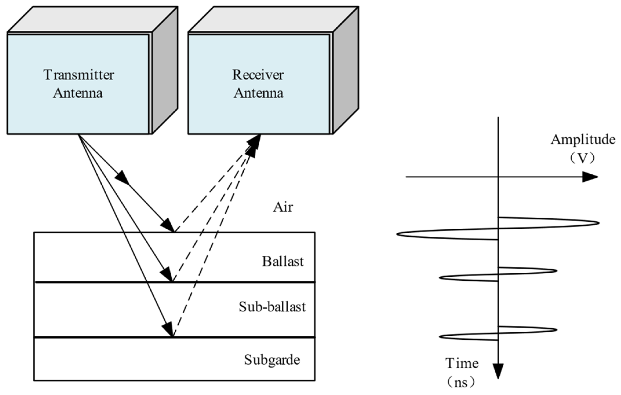
2.1. GPR Principles
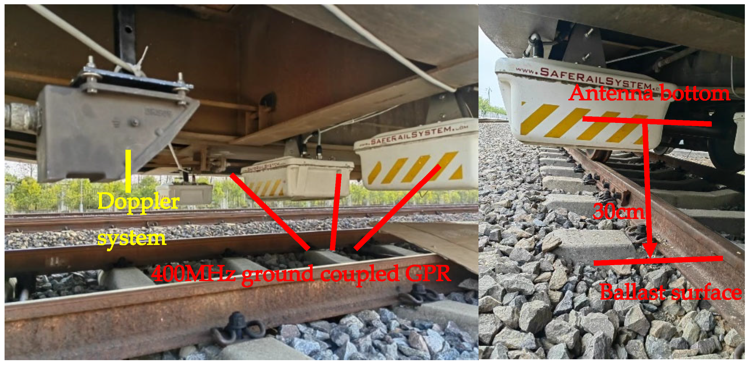
2.2. GPR Data Acquisition and Processing
- Sampling. Before filtering the original data, discrete sampling is required, and the sampling process needs to satisfy the sampling theorem; otherwise, the data spectrum will be mixed and thus generate false frequencies. The sampling theorem in the frequency domain equation is , where is the sampling frequency, is Nyquist frequency, and is the highest frequency of the signal [33].
- Zero-line correction. The zero-line setting is mainly carried out by cutting the air layer to a fixed threshold value, which is set at the most stable point on the electromagnetic wave trajectory A-scan. Depending on the type of antenna and the center frequency, setting the appropriate threshold position along the A-scan reflects the accuracy of the results, and this threshold can be summarized as (1) the initial arrival of the wave; (2) the position of the first trough; (3) the position of the first wave crest location of the zero amplitude value between the first wave crest and the trough; (4) the location of half the amplitude value between the first wave crest and the trough; (5) the position of the first wave crest [34].
- Gain setting. Using automatic gain control (AGC). When the signal is strong, its gain automatically decreases and when the signal is weak its gain automatically increases. It can ensure the uniformity of strong and weak signals and facilitate the tracking of effective waves [35].
- FIR bandpass filtering. The bandpass filter works by cutting off the fringe bands from the spectrum of GPR data. The filter consists of two filters, a high-pass filter and a low-pass filter, which modify the ground-penetrating radar signal by removing the low- and high-frequency components of the spectrum. As a rule of thumb, a bandwidth of 1.5 times the survey center frequency can be used initially [32,35].
- Running average filters. The background noise of the GPR signal is high, and the autoregressive sliding average spectral estimation (ARMA) in modern spectral estimation is used to analyze and identify the non-smooth signal of the effective reflected signal, which can extract the signal features at a low signal-to-noise ratio with a high accuracy of spectral estimation [36].
2.3. Training and Testing Dataset
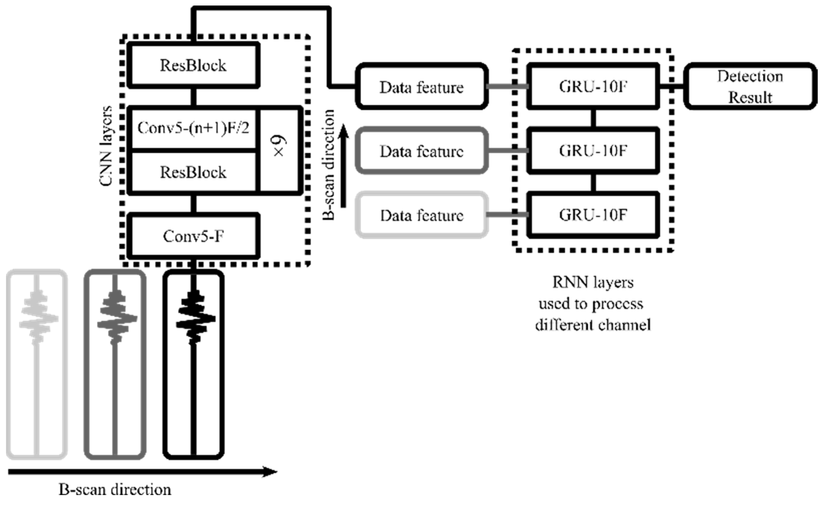
2.4. CRNN Network Structure
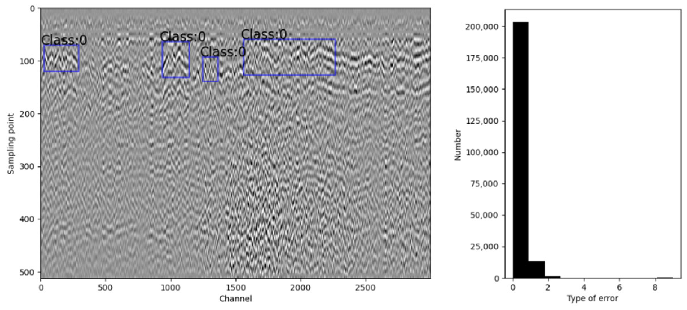
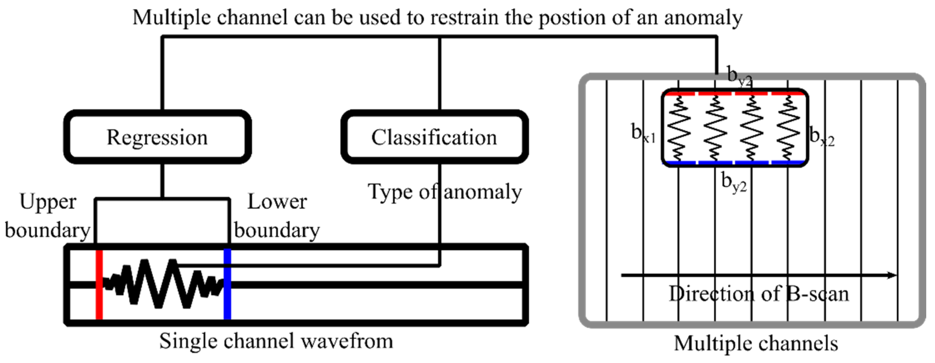
2.5. Anomaly Detection
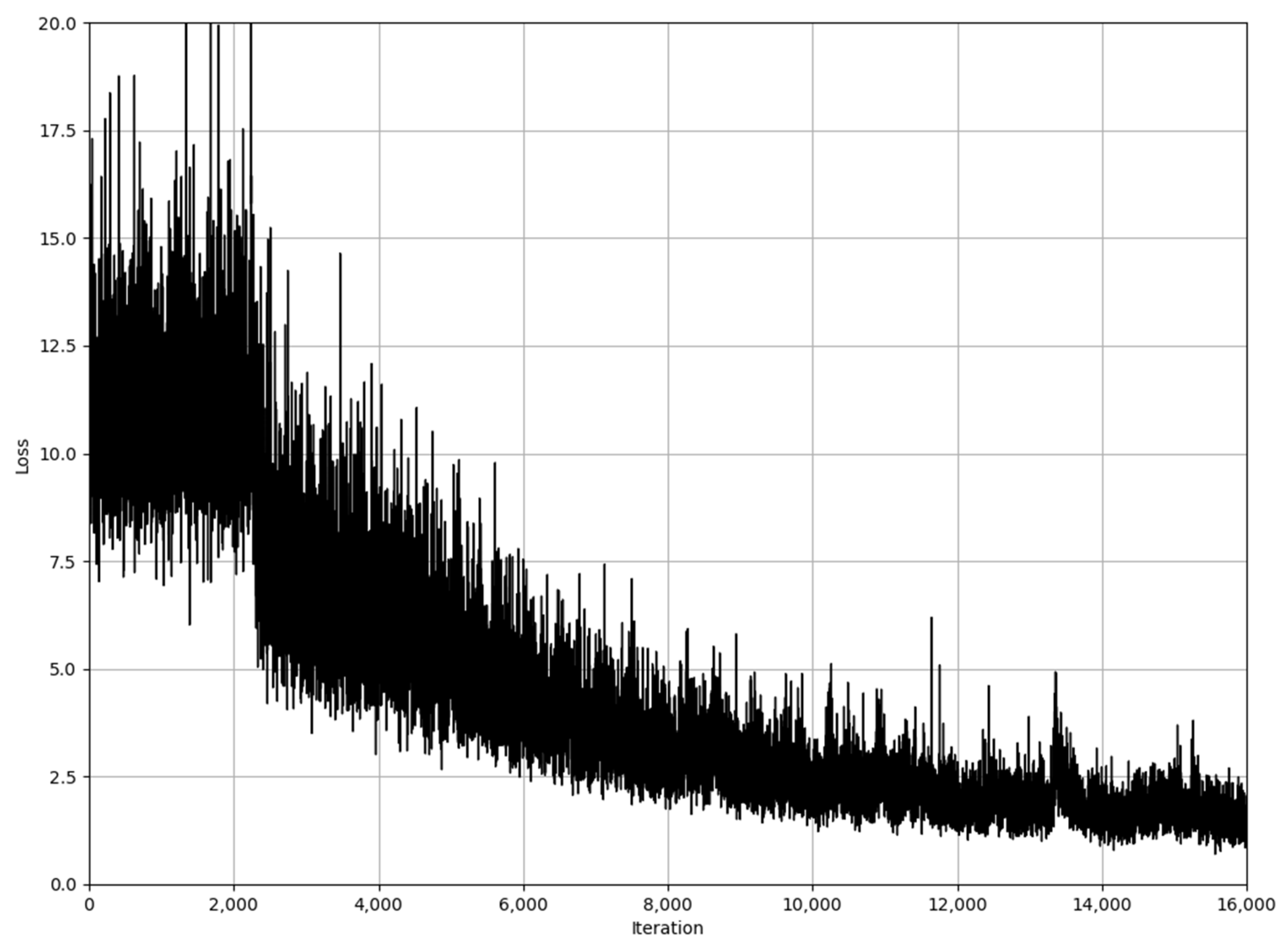
2.6. Training of CRNN
3. Case Study
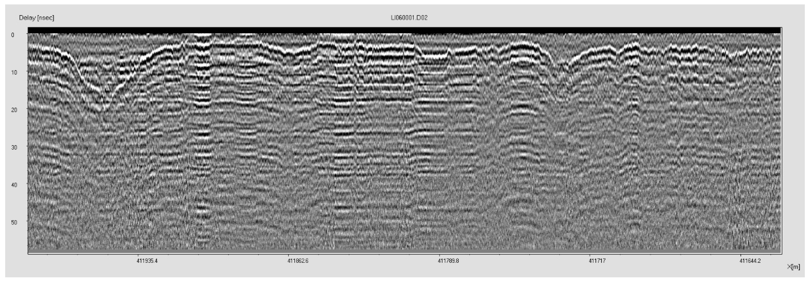
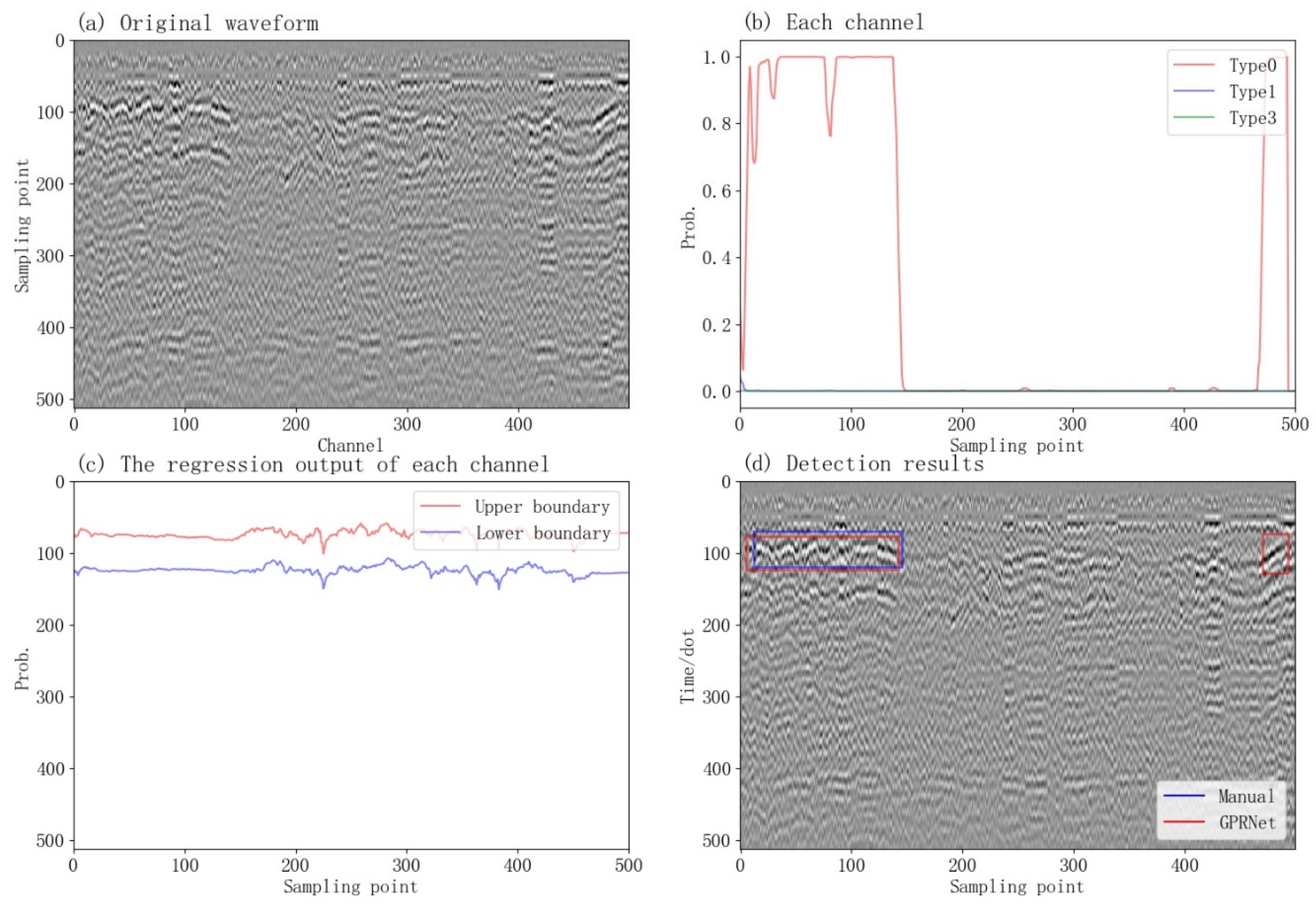
3.1. Detection Result on Real Railway Subgrade GPR Data
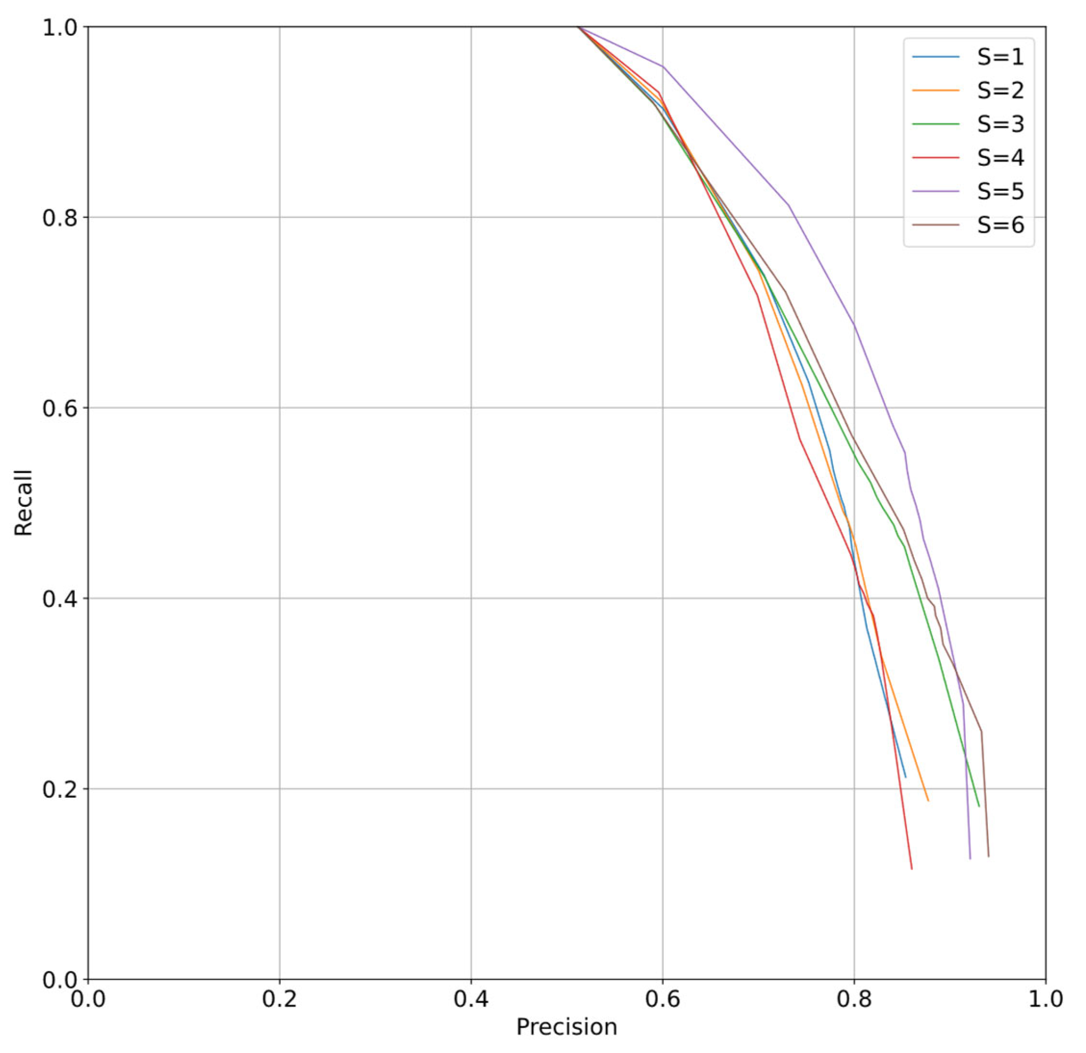
- Precision (P). This is the rate of successfully detected channels. It is calculated as .
- Recall (R). This is the rate of the detected anomalous channels out of all the anomalous channels in the dataset. It is calculated as .
- Mean error of the four boundaries. This indicates the bias of our model.
- The standard deviation of the four boundaries. This measures the variability in our model’s performance.
- The detection model is a single-way model.
3.2. The Inferring Speed in GPR Data
3.3. Comparison with Object Detection Models
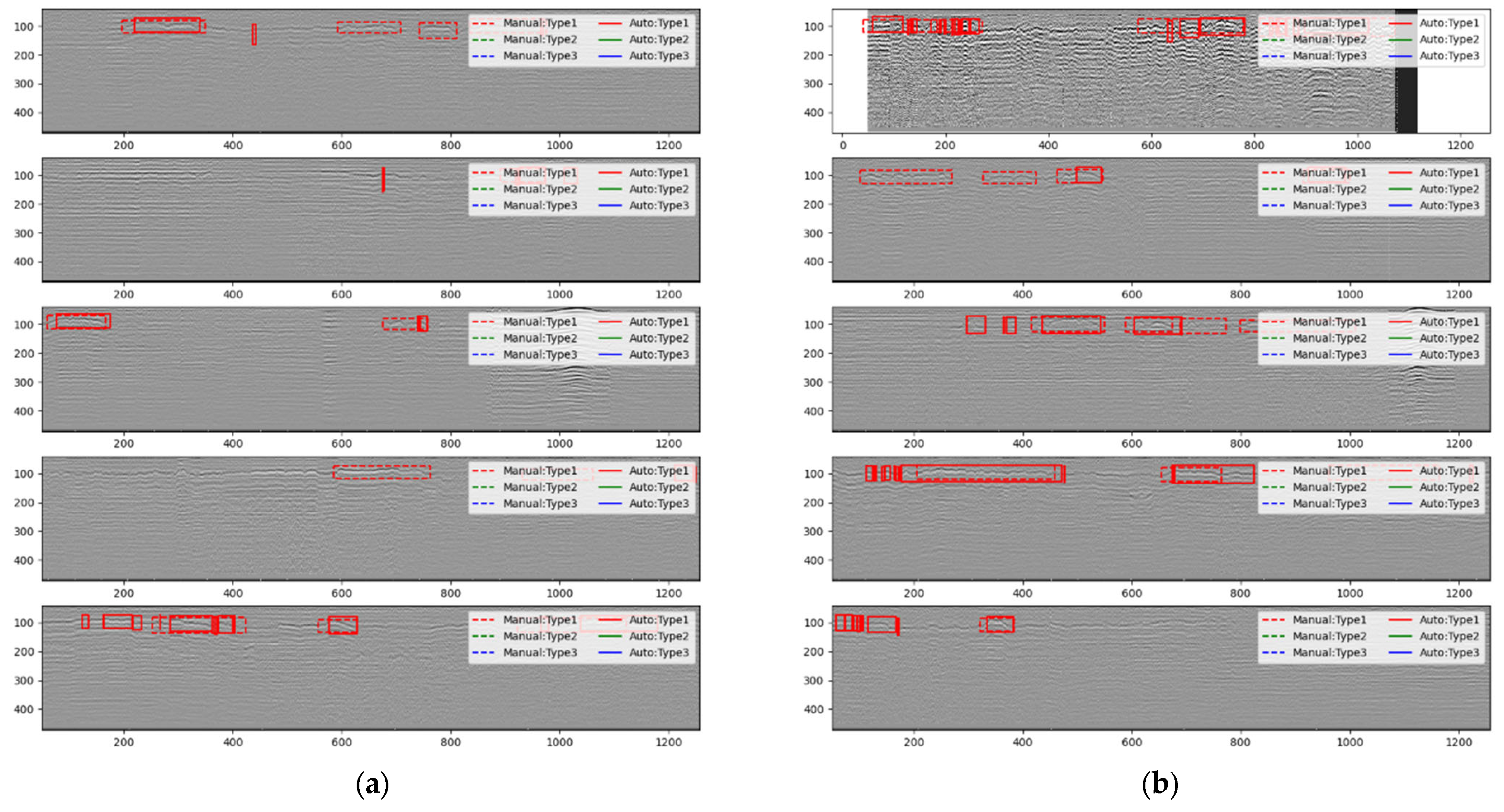
3.3.1. Detection Result on Image Data
3.3.2. Statics on Image Data
4. Conclusions and Perspective
Author Contributions
Funding
Institutional Review Board Statement
Informed Consent Statement
Data Availability Statement
Conflicts of Interest
References
- Wang, S.; Liu, G.; Jing, G.; Feng, Q.; Liu, H.; Guo, Y. State-of-the-Art Review of Ground Penetrating Radar (GPR) Applications for Railway Ballast Inspection. Sensors 2022, 22, 2450. [Google Scholar] [CrossRef] [PubMed]
- Fontul, S.; Paixão, A.; Solla, M.; Pajewski, L. Railway Track Condition Assessment at Network Level by Frequency Domain Analysis of GPR Data. Remote Sens. 2018, 10, 559. [Google Scholar] [CrossRef]
- Xiao, J.; Liu, L. Permafrost Subgrade Condition Assessment Using Extrapolation by Deterministic Deconvolution on Multifrequency GPR Data Acquired Along the Qinghai-Tibet Railway. IEEE J. Sel. Top. Appl. Earth Obs. Remote Sens. 2016, 9, 83–90. [Google Scholar] [CrossRef]
- Bano, M.; Tsend-Ayush, N.; Schlupp, A.; Munkhuu, U. Ground-Penetrating Radar Imaging of Near-Surface Deformation along the Songino Active Fault in the Vicinity of Ulaanbaatar, Mongolia. Appl. Sci. 2021, 11, 8242. [Google Scholar] [CrossRef]
- Solla, M.; Pérez-Gracia, V.; Fontul, S. A Review of GPR Application on Transport Infrastructures: Troubleshooting and Best Practices. Remote Sens. 2021, 13, 672. [Google Scholar] [CrossRef]
- Kang, M.-S.; Kim, N.; Lee, J.J.; An, Y.-K. Deep learning-based automated underground cavity detection using three-dimensional ground penetrating radar. Struct. Health Monit. 2020, 19, 173–185. [Google Scholar] [CrossRef]
- Manataki, M.; Vafidis, A.; Sarris, A. GPR Data Interpretation Approaches in Archaeological Prospection. Appl. Sci. 2021, 11, 7531. [Google Scholar] [CrossRef]
- Francke, J. Applications of GPR in mineral resource evaluations. In Proceedings of the XIII Internarional Conference on Ground Penetrating Radar, Lecce, Italy, 21–25 June 2010; pp. 1–5. [Google Scholar]
- Valles, J.; Chapa, T.; Matesanz, J.; González, M.A.M. Combined application of Multi-Channel 3D GPR and Photogrammetry from UAVs for the study of Archaeological sites. In Proceedings of the 3th Technoheritage 2017 International Congress, Cádiz, Spain, 20–23 May 2017; pp. 20–24. [Google Scholar]
- Lai, W.W.-L.; Dérobert, X.; Annan, P. A review of Ground Penetrating Radar application in civil engineering: A 30-year journey from Locating and Testing to Imaging and Diagnosis. NDT E Int. 2018, 96, 58–78. [Google Scholar]
- Liu, S.; Lu, Q.; Li, H.; Wang, Y. Estimation of Moisture Content in Railway Subgrade by Ground Penetrating Radar. Remote Sens. 2020, 12, 2912. [Google Scholar] [CrossRef]
- Shao, W.; Bouzerdoum, A.; Phung, S.L.; Su, L.; Indraratna, B.; Rujikiatkamjorn, C. Automatic classification of GPR signals. In Proceedings of the XIII Internarional Conference on Ground Penetrating Radar, Lecce, Italy, 21–25 June 2010; pp. 1–6. [Google Scholar]
- Du, C.; Zhang, Q.; Liu, J. Intelligent identification of railway roadbed defects by vector machines. In Proceedings of the 2017 Conference of China Civil Engineering Society, Guangzhou, China, 10–12 November 2017; pp. 355–365. (In Chinese). [Google Scholar]
- Hou, Z.; Zhao, W.; Yang, Y. Identification of railway subgrade defects based on ground penetrating radar. Sci. Rep. 2023, 13, 6030. [Google Scholar] [CrossRef]
- Alyoubi, K.H.; Sharma, A. A Deep CRNN-Based Sentiment Analysis System with Hybrid BERT Embedding. Int. J. Pattern Recognit. Artif. Intell. 2023, 37, 2352006. [Google Scholar] [CrossRef]
- Lee, K.; Lee, S.; Kim, H.Y. Deep Learning-Based Defect Detection Framework for Ultra High Resolution Images of Tunnels. Sustainability 2023, 15, 1292. [Google Scholar] [CrossRef]
- Zhang, L.; Zhang, K.; Pan, H. SUNet++: A Deep Network with Channel Attention for Small-Scale Object Segmentation on 3D Medical Images. Tsinghua Sci. Technol. 2023, 28, 628–638. [Google Scholar] [CrossRef]
- Gao, J.; Yuan, D.; Tong, Z.; Yang, J.; Yu, D. Autonomous pavement distress detection using ground penetrating radar and region-based deep learning. Measurement 2020, 164, 108077. [Google Scholar] [CrossRef]
- McLaughlin, N.; Del Rincon, J.M.; Miller, P. Recurrent Convolutional Network for Video-Based Person Re-identification. In Proceedings of the 2016 IEEE Conference on Computer Vision and Pattern Recognition (CVPR), Las Vegas, NV, USA, 27–30 June 2016; pp. 1325–1334. [Google Scholar]
- Tong, Z.; Gao, J.; Sha, A.; Hu, L.; Li, S. Convolutional Neural Network for Asphalt Pavement Surface Texture Analysis: Convolutional neural network. Comput.-Aided Civ. Infrastruct. Eng. 2018, 33, 1056–1072. [Google Scholar] [CrossRef]
- Besaw, L.E.; Stimac, P.J. Deep convolutional neural networks for classifying GPR B-scans. In Detection and Sensing of Mines, Explosive Objects, and Obscured Targets XX; Bishop, S.S., Isaacs, J.C., Eds.; SPIE Defense + Security: Baltimore, MD, USA, 2015; p. 945413. [Google Scholar]
- Xu, X.; Jiang, B.; Huang, Q. Intelligent identification method for railway roadbed slurry and mud infestation based on Cas-cade R-CNN. Railw. Eng. 2019, 29, 99–104. (In Chinese) [Google Scholar]
- Ma, Z.; Yang, F.; Qiao, X. Intelligent detection method for railway roadbed defects. Comput. Eng. Appl. 2021, 57, 272–278. (In Chinese) [Google Scholar]
- Tong, Z.; Gao, J.; Yuan, D. Advances of deep learning applications in ground-penetrating radar: A survey. Constr. Build. Mater. 2020, 258, 120371. [Google Scholar] [CrossRef]
- Xu, Y.; Kong, Q.; Huang, Q.; Wang, W.; Plumbley, M.D. Convolutional gated recurrent neural network incorporating spatial features for audio tagging. In Proceedings of the 2017 International Joint Conference on Neural Networks (IJCNN), Anchorage, AK, USA, 14–19 May 2017; pp. 3461–3466. [Google Scholar]
- Xie, F.; Lai, W.W.; Dérobert, X. Building simplified uncertainty models of object depth measurement by ground penetrating radar. Tunn. Undergr. Space Technol. 2022, 123, 104402. [Google Scholar] [CrossRef]
- Read, D.; Meddah, A.; Li, D.; Mui, W. Volpe Center. In Ground Penetrating Radar Technology Evaluation on the High Tonnage Loop: Phase 1: DOT/FRA/ORD-17/18; Federal Railroad Administration: Washington, DC, USA, 2017. [Google Scholar]
- Brown, M.; Li, D. Ground Penetrating Radar Technology Evaluation and Implementation: Phase 2: DOT/FRA/ORD-17/19; Federal Railroad Administration: Washington, DC, USA, 2017.
- Basye, C.; Wilk, S.; Gao, Y. Ground Penetrating Radar (GPR) Technology Evaluation and Implementation: DOT/FRA/ORD-20/18; Federal Railroad Administration: Washington, DC, USA, 2020.
- Shapovalov, V.; Vasilchenko, A.; Yavna, V.; Kochur, A. GPR method for continuous monitoring of compaction during the construction of railways subgrade. J. Appl. Geophys. 2022, 199, 104608. [Google Scholar] [CrossRef]
- Li, F.; Yang, F.; Yan, R.; Qiao, X.; Xing, H.; Li, Y. Study on Significance Enhancement Algorithm of Abnormal Features of Urban Road Ground Penetrating Radar Images. Remote Sens. 2022, 14, 1546. [Google Scholar] [CrossRef]
- Bianchini Ciampoli, L.; Tosti, F.; Economou, N.; Benedetto, F. Signal Processing of GPR Data for Road Surveys. Geosciences 2019, 9, 96. [Google Scholar] [CrossRef]
- Lombardi, F.; Griffiths, H.; Lualdi, M. The Influence of Spatial Sampling in GPR Surveys for the Detection of Landmines and IEDs. In Proceedings of the 2016 European Radar Conference (EuRAD), London, UK, 5–7 October 2016. [Google Scholar]
- Benedetto, A.; Tosti, F.; Ciampoli, L.B.; D’amico, F. An overview of ground-penetrating radar signal processing techniques for road inspections. Signal Process. 2017, 132, 201–209. [Google Scholar] [CrossRef]
- Jol, H.M. Ground Penetrating Radar: Theory and Application; Elsevier: Amsterdam, The Netherlands, 2009. [Google Scholar]
- Cui, F.; Wu, Z.-Y.; Wang, L.; Wu, Y.-B. Application of the Ground Penetrating Radar ARMA power spectrum estimation method to detect moisture content and compactness values in sandy loam. J. Appl. Geophys. 2015, 120, 26–35. [Google Scholar] [CrossRef]
- LeCun, Y.; Bengio, Y.; Hinton, G. Deep learning. Nature 2015, 521, 436–444. [Google Scholar] [CrossRef] [PubMed]
- Zhang, A.; Wang, K.C.; Li, B.; Yang, E.; Dai, X.; Peng, Y.; Fei, Y.; Liu, Y.; Li, J.Q.; Chen, C. Automated Pixel-Level Pavement Crack Detection on 3D Asphalt Surfaces with a Recurrent Neural Network: Automated pixel-level pavement crack detection on 3D asphalt surfaces using CrackNet-R. Comput.-Aided Civ. Infrastruct. Eng. 2019, 34, 213–229. [Google Scholar] [CrossRef]
- Mauch, L.; Yang, B. A new approach for supervised power disaggregation by using a deep recurrent LSTM network. In Proceedings of the 2015 IEEE Global Conference on Signal and Information Processing (GlobalSIP), Orlando, FL, USA, 14–16 December 2015; pp. 63–67. [Google Scholar]
- Glorot, X.; Bengio, Y. Understanding the difficulty of training deep feedforward neural networks. In Proceedings of the 13th International Conference on Artificial Intelligence and Statistics (AISTATS) 2010, Chia, Italy, 13–15 May 2010. [Google Scholar]
- Redmon, J.; Divvala, S.; Girshick, R.; Farhadi, A. You Only Look Once: Unified, Real-Time Object Detection. In Proceedings of the 2016 IEEE Conference on Computer Vision and Pattern Recognition (CVPR), Las Vegas, NV, USA, 27–30 June 2016; pp. 779–788. [Google Scholar]
- Kingma, D.P.; Ba, J. Adam: A Method for Stochastic Optimization. arXiv 2017, arXiv:1412.6980. [Google Scholar]
- Cho, K.; Van Merriënboer, B.; Bahdanau, D.; Bengio, Y. On the Properties of Neural Machine Translation: Encoder–Decoder Approaches. In Proceedings of the SSST-8, Eighth Workshop on Syntax, Semantics and Structure in Statistical Translation, Doha, Qatar, 25 October 2014; Association for Computational Linguistics: Doha, Qatar, 2014; pp. 103–111. [Google Scholar]
- Pascanu, R.; Mikolov, T.; Bengio, Y. On the difficulty of training Recurrent Neural Networks. arXiv 2013, arXiv:1211.5063. [Google Scholar]
- Ren, S.; He, K.; Girshick, R.; Sun, J. Faster R-CNN: Towards Real-Time Object Detection with Region Proposal Networks. IEEE Trans. Pattern Anal. Mach. Intell. 2017, 39, 1137–1149. [Google Scholar] [CrossRef]
- Hou, F.; Rui, X.; Fan, X.; Zhang, H. Review of GPR Activities in Civil Infrastructures: Data Analysis and Applications. Remote Sens. 2022, 14, 5972. [Google Scholar] [CrossRef]


| Railway Subgrade Defect Types | Typical Defects Image | Image Features |
|---|---|---|
| Normal subgrade without defect |  | The lamellar structure is obvious. The in-phase axis is straight and continuous. The reflected energy is uniform. |
| Mud pumping |  | The wave group is a disorganized, discontinuous, low-frequency strong reflection shape that resembles a mountain tip or straw hat. |
| Settlement |  | The reflection of the in-phase axis of the settlement radar image is significantly bent, with depth-downward offset. |
| Water anomaly |  | The signal is attenuated. The reflected energy of the top surface is strong. Multiple waves exit. |
| Model | P | R | ||||
|---|---|---|---|---|---|---|
| S = 1 | 0.79 | 0.74 | −14.73 | −40.47 | 30.25 | 48.59 |
| S = 2 | 0.79 | 0.7 | −17.67 | −44.56 | 31.05 | 50.98 |
| S = 3 | 0.79 | 0.71 | −18.13 | −42.86 | 30.4 | 49.75 |
| S = 4 | 0.81 | 0.67 | −20.74 | −47.71 | 32.06 | 52.6 |
| S = 5 | 0.76 | 0.73 | −16.38 | −39.54 | 28.87 | 48.58 |
| S = 6 | 0.76 | 0.65 | −22.41 | −50.83 | 31.3 | 52.39 |
| Running Device | Inferring Time (ms) |
|---|---|
| CPU | 1325 |
| GPU | 2139 |
| Model Name | Faster RCNN | CRNN (Ours) | ||||
|---|---|---|---|---|---|---|
| Precision | Recall | F1Score | Precision | Recall | F1Score | |
| IoU > 0.25 | 0.777 | 0.936 | 0.849 | 0.795 | 0.941 | 0.862 |
| IoU > 0.50 | 0.752 | 0.671 | 0.709 | 0.834 | 0.773 | 0.803 |
| IoU > 0.75 | 0.527 | 0.260 | 0.348 | 0.422 | 0.158 | 0.230 |
| Model Name | Faster RCNN | CRNN (Ours) |
|---|---|---|
| Detected 238 images on CPU (ms) | 18,000 | 2600 |
| Detected 238 images on GPU (ms) | 2000 | 500 |
| Model Size (MB) | 104 | 2.6 |
| Deep Model | Advantages | Disadvantages |
|---|---|---|
| CNN | One-dimensional CNN can extract features in-depth, i.e., longitudinally, in the time dimension, generating a vector for each GPR waveform which can reduce the storage requirements [19]. | Since CNN has no memory function for time series, it cannot take the input data sequence into account like RNN [24]. |
| RNN | RNN can be regarded as a series of interconnected networks that have a chained architecture, where the output of the next network depends on both its input and the output of its predecessor network [43]. | Because of the chain derivative rule and the existence of a nonlinear activation function, RNN is prone to the problem of gradient vanishing and explosion [44]. |
| CRNN | Lightweight, the model size is only 2.6 MB. Faster inference speeds on both CPU and GPU are easy to deploy on hardware devices. No complex data processing steps are required (e.g., filtering and information compression), taking into account the physical mechanisms of GPR data and their temporal dynamic behavior. | Due to the insufficient sample number and sample imbalance, the CRNN model only determines the existence of anomalous regions, and the identified anomalies still need to be interpreted manually. When the IoU is greater than 0.75, the accuracy of the CRNN model is low, and more neurons may need to be added to improve accuracy. |
| Faster R-CNN | Faster RCNN, as a two-stage network, contains RPN and RCNN, and has higher recognition accuracy compared to the one-stage network. Many deep learning frameworks have a practical [45] Faster RCNN source code that is easy to use. | Although the detection accuracy of Faster RCNN is improved, the training speed of its network model is slow [46]. |
Disclaimer/Publisher’s Note: The statements, opinions and data contained in all publications are solely those of the individual author(s) and contributor(s) and not of MDPI and/or the editor(s). MDPI and/or the editor(s) disclaim responsibility for any injury to people or property resulting from any ideas, methods, instructions or products referred to in the content. |
© 2023 by the authors. Licensee MDPI, Basel, Switzerland. This article is an open access article distributed under the terms and conditions of the Creative Commons Attribution (CC BY) license (https://creativecommons.org/licenses/by/4.0/).
Share and Cite
Liu, H.; Wang, S.; Jing, G.; Yu, Z.; Yang, J.; Zhang, Y.; Guo, Y. Combined CNN and RNN Neural Networks for GPR Detection of Railway Subgrade Diseases. Sensors 2023, 23, 5383. https://doi.org/10.3390/s23125383
Liu H, Wang S, Jing G, Yu Z, Yang J, Zhang Y, Guo Y. Combined CNN and RNN Neural Networks for GPR Detection of Railway Subgrade Diseases. Sensors. 2023; 23(12):5383. https://doi.org/10.3390/s23125383
Chicago/Turabian StyleLiu, Huan, Shilei Wang, Guoqing Jing, Ziye Yu, Jin Yang, Yong Zhang, and Yunlong Guo. 2023. "Combined CNN and RNN Neural Networks for GPR Detection of Railway Subgrade Diseases" Sensors 23, no. 12: 5383. https://doi.org/10.3390/s23125383
APA StyleLiu, H., Wang, S., Jing, G., Yu, Z., Yang, J., Zhang, Y., & Guo, Y. (2023). Combined CNN and RNN Neural Networks for GPR Detection of Railway Subgrade Diseases. Sensors, 23(12), 5383. https://doi.org/10.3390/s23125383