1. Introduction
Ever-increasing demand and congestion on existing road networks necessitates effective transportation planning, design, and management. This informed decision making requires accurate traffic data. Most medium- to long-term traffic planning and modeling is focused on traffic demand, as quantified by traffic counts or flow. Traffic flow is generally measured by fixed-location counting, which can be accomplished using permanent detectors or, in many cases, temporary detectors or human observers. Many traditional traffic studies use temporary pneumatic tube or inductive loop technologies that are deployed for only a few days at each location, and each location is revisited only every three to five years. So, while traffic flow measurement is key to estimating demand throughout the network, the available data are spatially and temporally sparse and often out of date.
A large body of work has focused on automatic vision-based traffic surveillance with stationary cameras [
1,
2,
3,
4,
5,
6,
7]. More recently, state-of-the-art vehicle detection performance has appreciably improved with Convolutional Neural Network (CNN)-based mature 2D object detectors such as Mask-RCNN [
8], Yolo v3 [
9], and Yolo v4 [
10]. These models are feasible to deploy in real time. For most surveillance tasks, a processing rate of 4–5 frames per second is sufficient [
11], which is achievable with these detectors. However, stationary, fixed-location cameras cannot cover the entirety of the road network.
Unmanned Aerial Vehicle (UAV) based automatic traffic surveillance [
12,
13,
14,
15] is a good alternative to stationary cameras. Drones can monitor a larger part of the network and track vehicles across multiple segments. However, UAV operation carries its own technical and regulatory limitations. Adverse climate affects flight dynamics substantially [
15], and vehicle detection suffers from the lower resolution of camera views at higher flight elevations.
Recent studies proposed and developed the concept that public transit bus fleets could be used as surveillance agents [
16,
17,
18]. Transit buses tend to operate on roadways with a greater concentration of businesses, residences, and people, and so they often cover many of the more heavily used streets that would be selected for a traditional traffic study. As discussed in the above noted studies, this method could also be deployed on other municipal service vehicles that might already be equipped with cameras; however, one advantage of using transit buses is that their large size allows cameras to be mounted higher above the ground, thus reducing the occurrence of occlusions.
Prior work on measuring traffic flow from moving vehicles has relied on manual counts or used dedicated probe vehicles equipped with lidar sensors [
16,
17]. Lidar sensors were used because the automatic processing of lidar data is readily achievable. However, unlike lidar, video sensors are already deployed on transit buses for liability, safety, and security purposes. The viability, validity, and accuracy of the use of video imagery recorded by cameras mounted on transit buses was established by manually counting vehicles captured in this imagery with the aid of a graphical user interface (GUI) [
18]. However, for practical large-scale applications, the processing of video imagery and the counting of vehicles must be fully automated.
In this paper, we propose to operationalize this traffic surveillance methodology for practical applications, leveraging the perception and localization sensors already deployed on these vehicles. This paper develops a new, automatic, vision-based vehicle counting method applied to the video imagery recorded by cameras mounted on transit buses. To the best of our knowledge, this paper is the first effort to apply automated vision-based vehicle detection and counting techniques to video imagery recorded from cameras mounted on bus-transit vehicles.
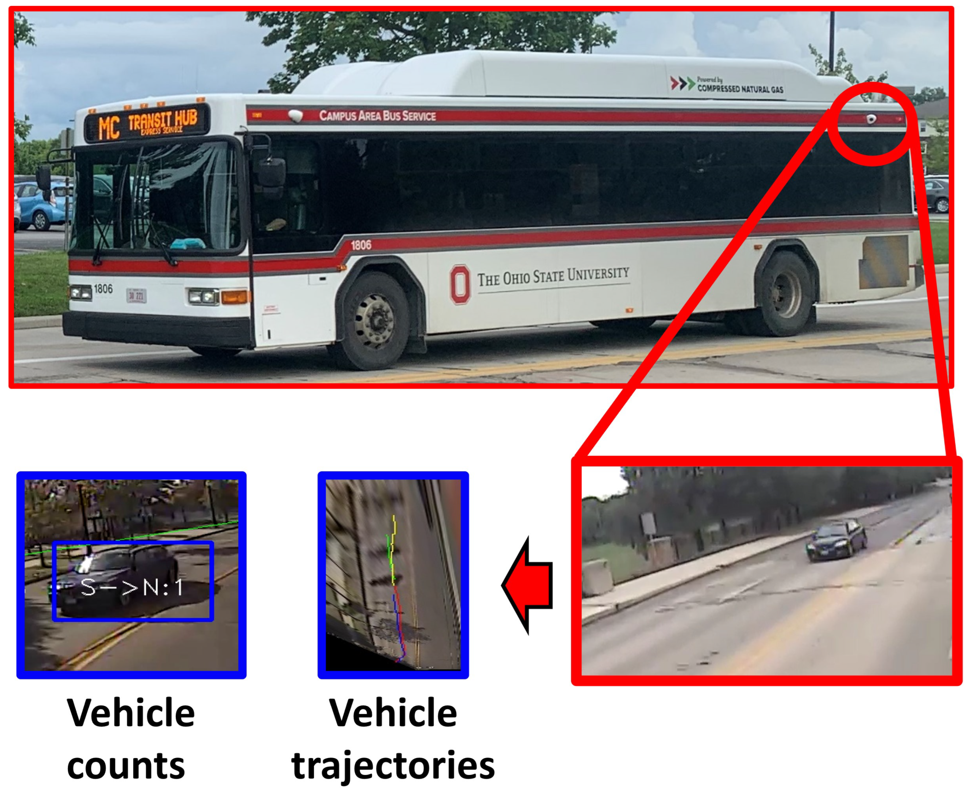
Figure 1 shows an example deployment of cameras on a transit bus, including example video imagery. This configuration is used in the experiments presented in this paper. By fully automating the vehicle counting process, this approach offers a potentially low-cost method to extend surveillance to considerably more of the traffic network than fixed-location sensors currently provide, while also providing more timely updates than temporary traffic study sensor deployments.
The main contributions of this study are the following:
An automatic vision-based vehicle counting and trajectory extraction method using video imagery recorded by cameras mounted on transit buses.
A real-world demonstration of the automated system and its validation using video from in-service buses. An extensive ablation study was conducted to determine the best components of the pipeline, including comparisons of state-of-the-art CNN object detectors, Kalman filtering, deep-learning-based trackers, and region-of-interest (ROI) strategies.
The main challenges in this endeavor are as follows: estimating vehicle trajectories from a limited observation window, robust vehicle detection and tracking while moving, localizing the sensor platform, and differentiating parked vehicles from traffic participants.
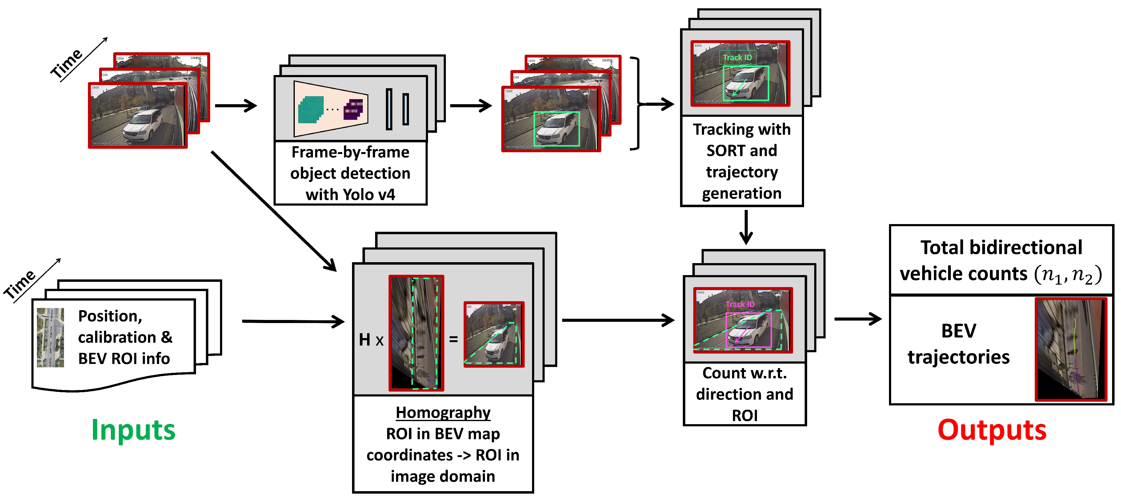
Figure 2 shows an overview of the processing pipeline. First, images obtained from a monocular camera stream are processed with the automatic vehicle counter developed in this study. A Yolo v4 [
10] deep CNN trained on the MS COCO dataset [
19] detects vehicles, while SORT [
20], a Kalman filter and Hungarian algorithm based tracker which solves an optimal assignment problem, generates unique tracking IDs for each detected vehicle. Next, using subsequent frames, the trajectory of each detected vehicle is projected onto the ground plane with a homographic perspective transformation. Then, each trajectory inside a predefined, geo-referenced region-of-interest (ROI) is counted with a direction indicator. The automatic vehicle counts are compared against human-annotated ground-truth counts for validation. In addition, an exhaustive ablation study is conducted to determine the best selection of 2D detectors, trackers, and ROI strategies.
3. Method
As mentioned previously, our work focuses solely on automatically obtaining vehicle counts and extracting trajectories using computer vision. What follows are detailed descriptions of the problem and the various steps of the developed methodology.
3.1. Problem Formulation
Given an observation at time t as , where is an image captured by a monocular camera mounted on the bus and is the position of the bus on a top-down 2D map, the first objective is to find , a function that maps a sequence of observations to the total number of vehicles counted traveling in each direction . The second objective is to find , which provides the m tuples of detected vehicles’ trajectories. The trajectory of detected vehicle i is given with , where J is the total number of frames in which vehicle i was observed by the bus and is the bird’s-eye-view real-world position vector of vehicle i.
The overview of the solution is shown in
Figure 2. The proposed algorithm, Detect-Track-Project-Count (DTPC), is given in Algorithm 1. The implementation details of the system are presented in
Section 4.
| Algorithm 1: Detect-Track-Project-Count: DTPC() |
 |
3.2. Two-Dimensional Detection
A vehicle detection D is defined as , where contains the bounding box corners in pixel coordinates, l is the class label (e.g., car, bus, or truck), and c is the confidence of the detection. A 2D CNN maps each image captured by the bus camera to q tuples of detections D. This processing is performed on individual image frames. The object classification information is used to avoid counting pedestrians and bicycles but could also be used in other studies.
The networks commonly known as Mask-RCNN [
8], Yolo v3 [
9], and Yolo v4 [
10], pretrained on the MS COCO dataset [
19], are employed for object detection. Based on the ablation study presented subsequently, the best-performing detector was identified as Yolo v4.
3.3. Tracking
The goal of tracking is to associate independent frame-by-frame detection results across time. This step is essential for trajectory extraction, which is needed in order to avoid counting the same vehicle more than once.
SORT [
20], a fast and reliable algorithm that uses Kalman filtering and the Hungarian algorithm to solve the assignment problem, is employed for the tracking task. First, define the state vector as
where
and
are the bounding box center coordinates derived from the resultant 2D detection bounding boxes,
is its area,
is its aspect ratio, and
and
are the corresponding first derivatives with respect to time.
The next step consists of associating each detection to already existing target boxes with unique tracking IDs. This subproblem can be formulated as an optimal assignment matching problem where the matching cost is the Intersection-over-Union (IoU) value between a detection box and a target box i.e.,
This problem can be solved with the Hungarian algorithm [
45].
After each detection is assigned to a target, the target state is updated with a Kalman filter [
46]. The Kalman filter assumes the following dynamical model:
where,
is the state transition matrix,
is the control input matrix,
is the control vector, and
is normally distributed noise. The Kalman filter recursively estimates the current state from the previous state and the current actual observation as follows:
where
P is the predicted covariance matrix and
Q is the covariance of the multivariate normal noise distribution. Details of the update step can be found in the original Kalman filter paper [
46].
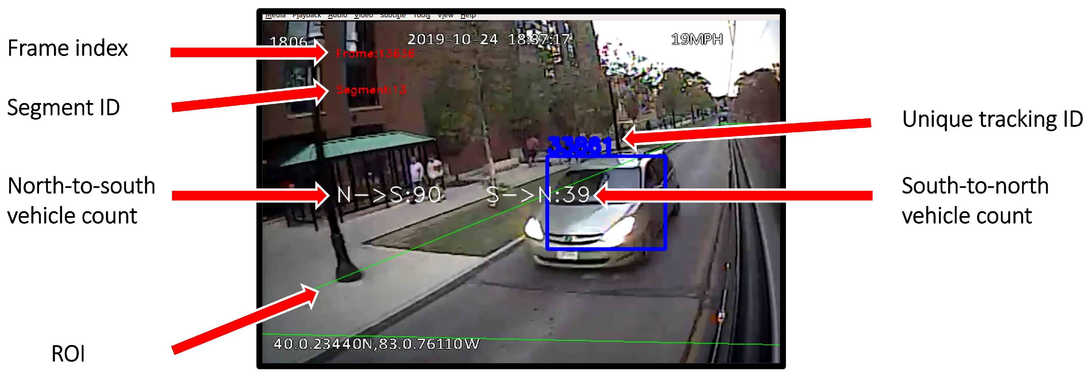
Deep SORT [
23] was also considered as an alternative to SORT [
20]; however, SORT gave better results. An example of a detected, tracked, and counted vehicle is shown in
Figure 3.
3.4. Geo-Referencing and Homography
The proposed method utilizes geo-referencing and homographic calibration to count vehicles in the desired ROI and transforms the detected vehicles’ trajectories from pixel coordinates to real-world coordinates.
GNSS measurement data are used to localize the bus with a pose vector at time t. A predefined database contains geo-referenced map information about the road network and divides each road into road segments with a predefined geometry, including the lane widths for each segment. Road segments tend to run from one intersection to another but can also be divided at points where the road topology changes significantly, for example, when a lane divides. This information is used to build the ROI in BEV real-world coordinates for each road segment.
The pixel coordinates of each detection can be transformed into real-world coordinates with planar homography using
since planar homography is up-to-scale with a scaling factor.
H, the homography matrix, has eight degrees of freedom. Hence,
H can be determined from four real-world image point correspondences [
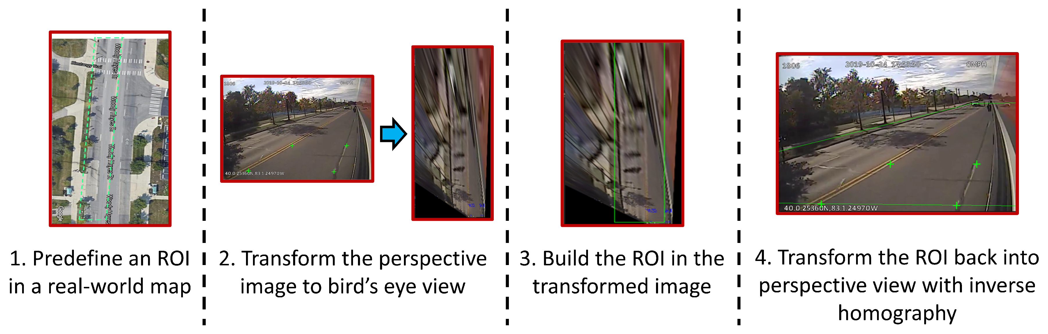
47]. Finding four point correspondences is fairly straightforward for urban road scenes. Standard road markings and the width of a lane are used to estimate
H. The homographic calibration process is shown in
Figure 4.
Once H is obtained, the inverse projection can be easily achieved with the inverse homography matrix . Inverse homography is used to convert a BEV real-world ROI to a perspective ROI for the image plane. After obtaining the perspective ROI, vehicles on the corresponding regions can be counted.
3.5. Counting
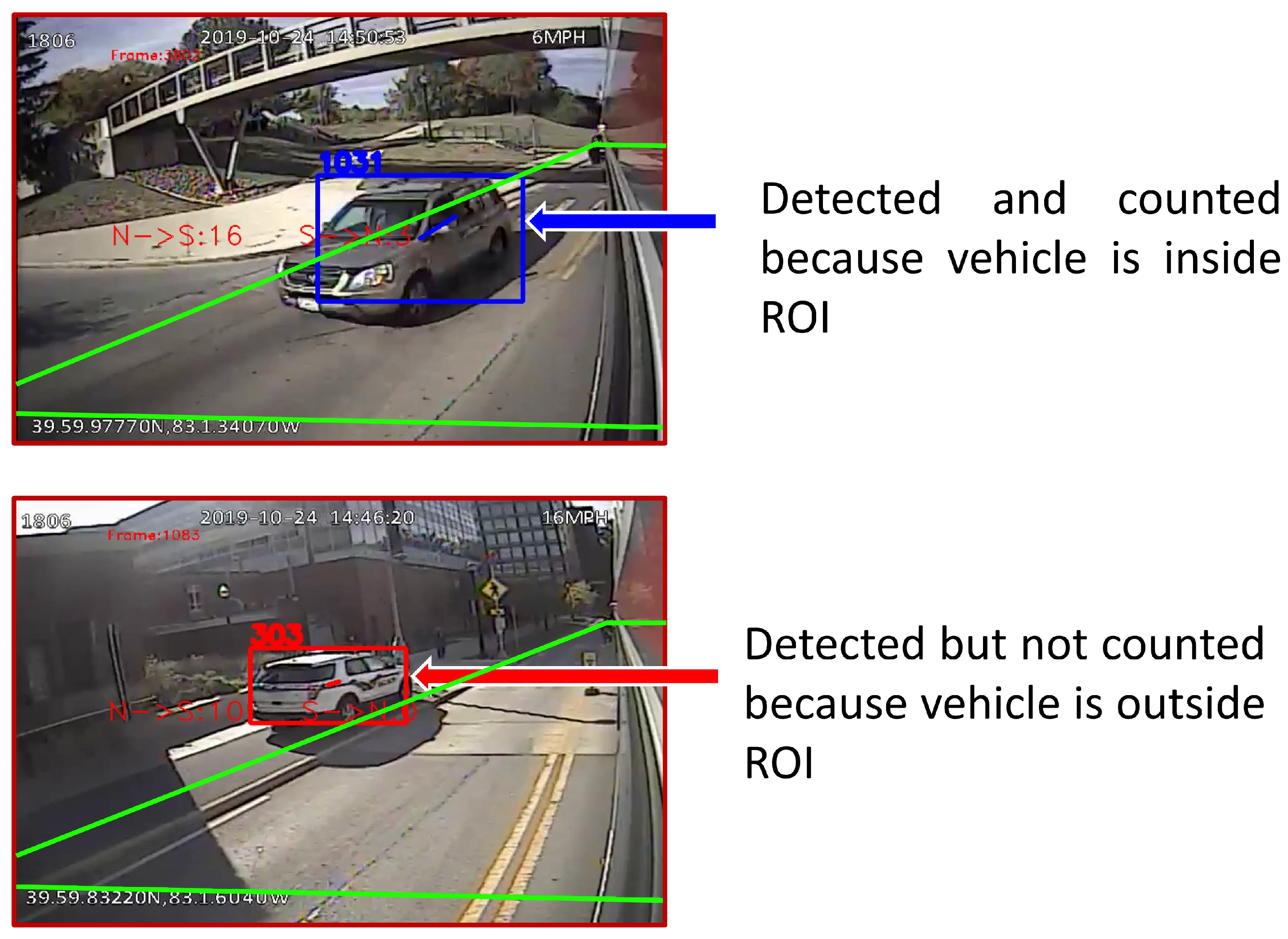
The objective of counting is to count each unique tracked vehicle once if it is a traffic participant and not a parked vehicle, travels in the corresponding travel direction, and is within the ROI.
The 2D object detector’s output is considered only if the inferred class
l =
and the bounding box center is within the ROI. Thus, at each counting time
t, using
and
, the bounding box center coordinates of each tracked vehicle
i, the count in the top-to-bottom direction (i.e., opposite the direction of travel of the bus) is updated incrementally
if the one-step sequence
of the image domain trajectory of vehicle
i satisfies
and vehicle
i was not counted before. In a similar fashion, the count in the bottom-to-top direction (i.e., in the direction of travel of the bus) is updated incrementally
if
and vehicle
i was not counted before. The ROI alignment for counting purposes is shown in steps 3 and 4 of
Figure 4.
Distinguishing parked vehicles from traffic flow participants is achieved by the ROI. This distinction and the difference between detecting and counting vehicles is illustrated in
Figure 5.
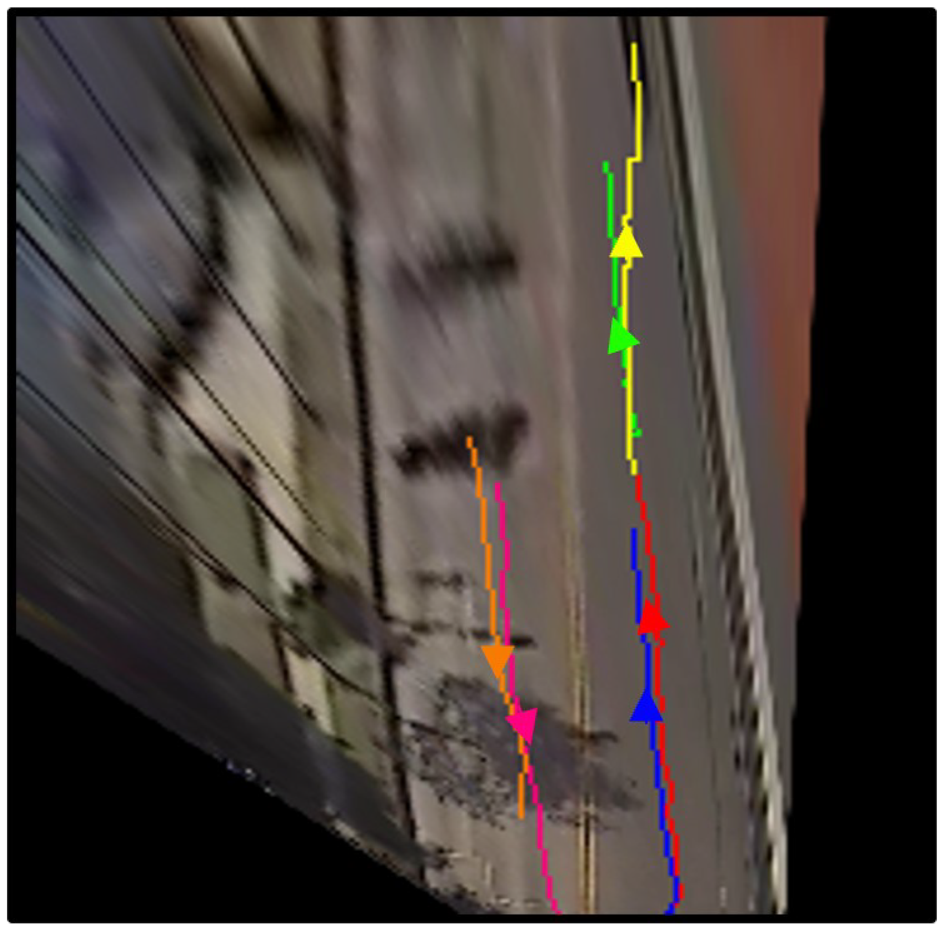
3.6. Trajectory Extraction in BEV Real-World Coordinates
Finally, for each tracked unique vehicle, a trajectory in BEV real-world coordinates relative to the bus is built by transforming the image-domain coordinates using the inverse homography projection. The image domain trajectory of vehicle
i,
, is transformed into
, with inverse homography,
. An example of extracted trajectories is illustrated in
Figure 6.
Trajectory extraction in BEV real-world coordinates is not strictly necessary for the purpose of counting unique vehicles, which could be achieved without such transformation. However, it is quite valuable for understanding the continuous behavior of traffic participants, including their speed, and therefore could be used as input to other studies.
4. Experimental Evaluation
4.1. Transit Bus
The Ohio State University owns and operates the Campus Area Bus Service (CABS) system consisting of a fleet of about 50 40-foot transit buses that operate on and in the vicinity of the OSU campus, serving around five million passengers annually (pre-COVID-19). As is the case for many transit systems, the buses are equipped with an Automatic Vehicle Location (AVL) system that includes GNSS sensors for operational and real-time information purposes and several interior- and exterior-facing monocular cameras that were installed for liability, safety, and security purposes. The proposed method depends on having an external view angle wide enough to capture the motion pattern of the surrounding vehicles.
Figure 3,
Figure 4 and
Figure 5 show sample image frames recorded by these cameras.
Video imagery collected from CABS buses while in service are used to implement and test the developed method. We chose to use the left side-view camera in this study because it is mounted higher than the front-view camera, which both reduces the potential for occlusions caused by other vehicles and improves the view of multiple traffic lanes to the side of the bus, particularly on wider multilane roads or divided roads with a median. Moreover, video from these cameras is captured at a lower resolution, which significantly reduces the size of the video files that needed to be offloaded, transferred, and stored. The video footage was recorded at 10 frames per second with a resolution of 696 × 478.
4.2. Implementation Details
The proposed algorithm was implemented in Python using OpenCV, Tensorflow, and Pytorch libraries. For 2D detectors, the original implementations of Mask-RCNN [
8], Yolo v3 [
9], and Yolo v4 [
10] were used. All models were pretrained on the MS COCO dataset [
19]. Experiments were conducted with an NVIDIA RTX 2080 GPU.
High-speed real-time applications are not within the scope of this study. For surface road traffic surveillance purposes, low frame rates are sufficient. The video files used in this study were downloaded from the buses after they complete their trips. However, it would be possible to perform the required calculations using edge computing installed on the bus or even integrated with the camera. This is a topic for future study.
4.3. Data Collection and Annotation
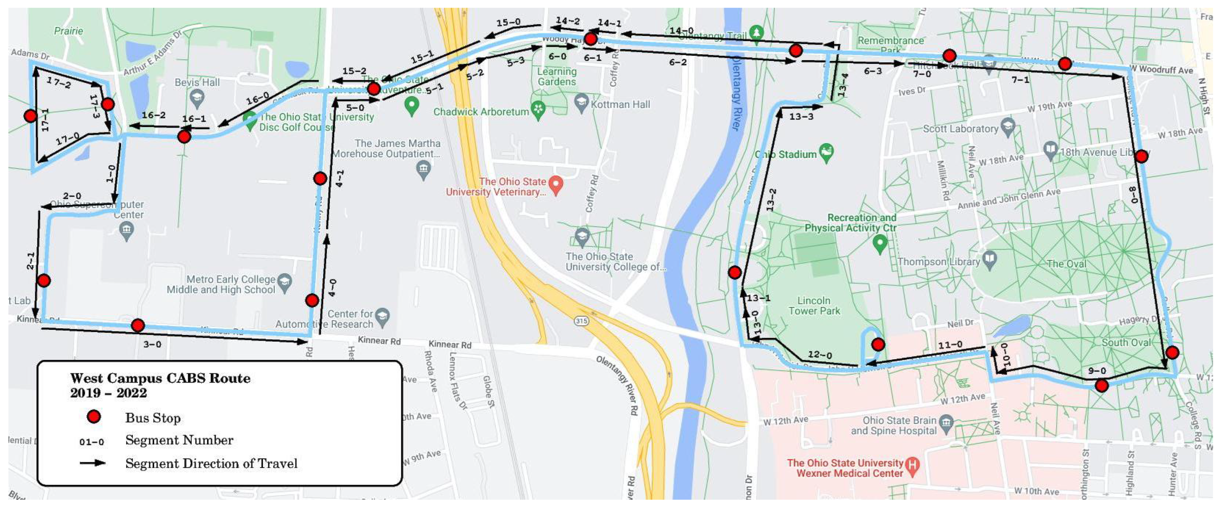
A total of 3.5 hours of video footage, collected during October 2019, was used for the experimental evaluation of the ablation study. An additional 3 hours of video footage, collected during March 2022, was used for the evaluation of the impacts of adverse weather. The West Campus CABS route on which the footage was recorded traverses four-lane and two-lane public roads. The route is shown in
Figure 7. As described above, this route was divided into road segments which tend to run from one intersection to another but may be divided at other points, such as when the road topology changes significantly. This can include points at which the number of lanes change or, in the case of this route, areas in which a tree-lined median strip obscures the camera view. Using this map database, sections with a tree-lined median strip and occlusions were excluded from the study. For each road segment, an ROI was defined with respect to road topology and lane semantics to specify the counting area. As a result, a total of 55 bus pass and roadway segment combinations were used in the ablation study evaluation analysis.
We note that should the bus not follow its prescribed route or the route changes, the algorithm can detect and report this due to the map database, as well as remove or ignore those portions of traveled road that are off-route or for which the road geometry information needed to form an ROI is not available.
The video footage was processed by human annotators in order to extract ground-truth vehicle counts. Annotators used a GUI to incrementally increase the total vehicle count for each oncoming unique vehicle and to capture the corresponding video frame number. Annotators counted vehicles once and only if the vehicle passed a virtual horizontal line drawn on the screen of the GUI while traveling in the direction opposite to that of the bus.
After annotation, the video frames, counts, and GNSS coordinates were synchronized for comparison with the results of the developed image-processing-based fully automated method.
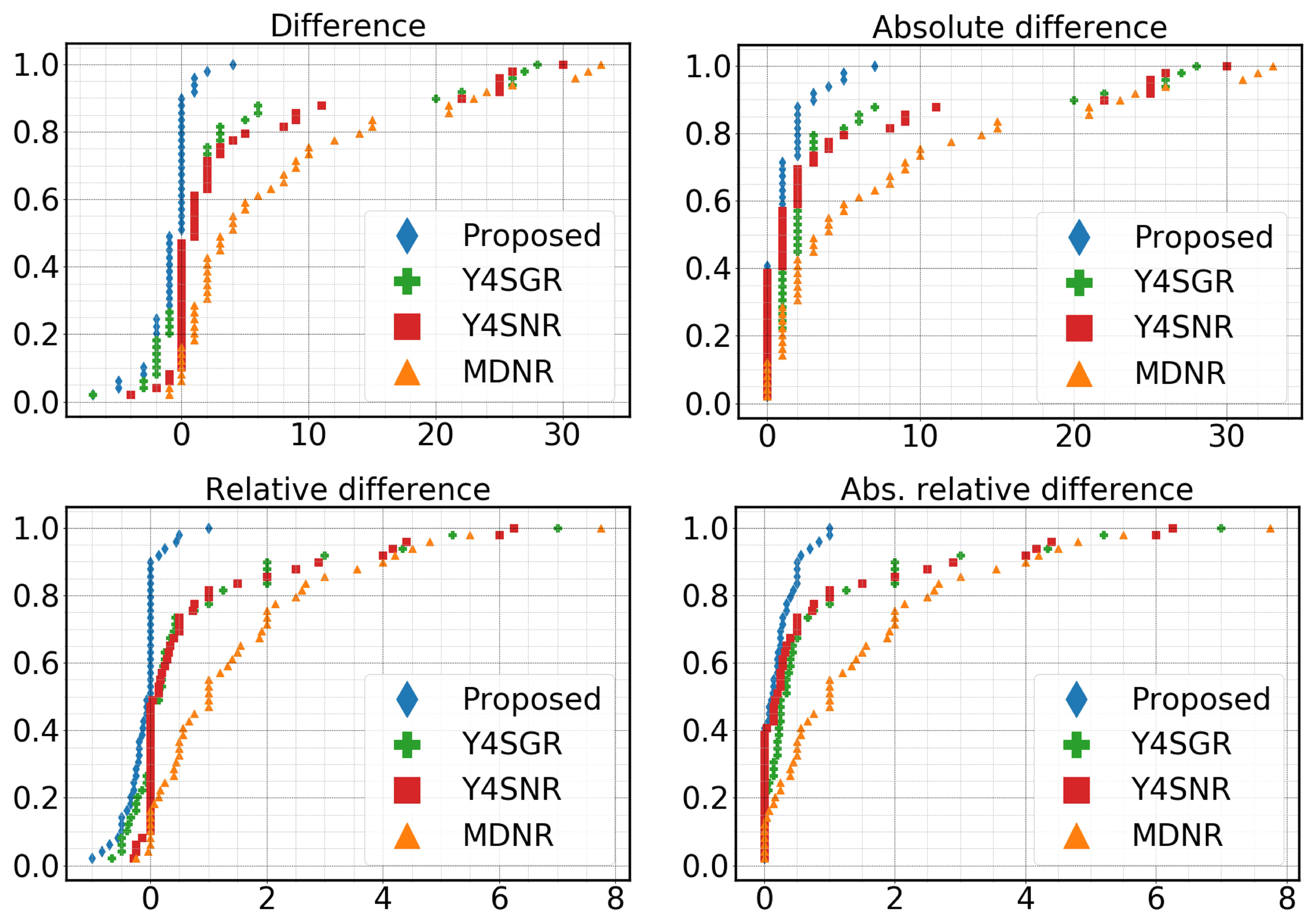
4.4. Evaluation Metrics
First, for each of the 55 bus pass and segment combination, ground-truth counts and inferred counts using the developed automatic counting method were compared with one another. In addition to examining a scatter plot that depicts this comparison, four metrics were considered, namely difference , absolute difference , absolute relative difference , and relative difference , where is the ground-truth count, and is the inferred count.
The sample mean, sample median, and empirical Cumulative Distribution Function (eCDF) were calculated for the proposed and alternative automated baseline methods.
4.5. Ablation Study
An extensive ablation study was conducted to identify the best alternative among multiple methods that could be applied to each phase of the counting system. All the combinations of modules from the following list were compared with one another using the sample mean and sample median of the evaluation metrics to find the better performing combinations:
The Generic ROI was defined based on a standard US two-lane road in perspective view. Each combination option is denoted by the sequence of uppercase first letters of the name of the modules. For example, Y4SGR stands for the Yolo 4 detector, SORT tracker, and Generic ROI combination. The proposed method is denoted with “Proposed” and stands for the Yolo 4 detector, SORT tracker, and Dynamic ROI combination.
5. Results and Discussion
5.1. Ablation study
Considering all combinations of tools, the proposed method, consisting of the Yolo v4 object detector, SORT tracker, and Dynamic Homography ROI, was found to be the best based on the sample mean, sample median, and eCDF of the four evaluation metrics.
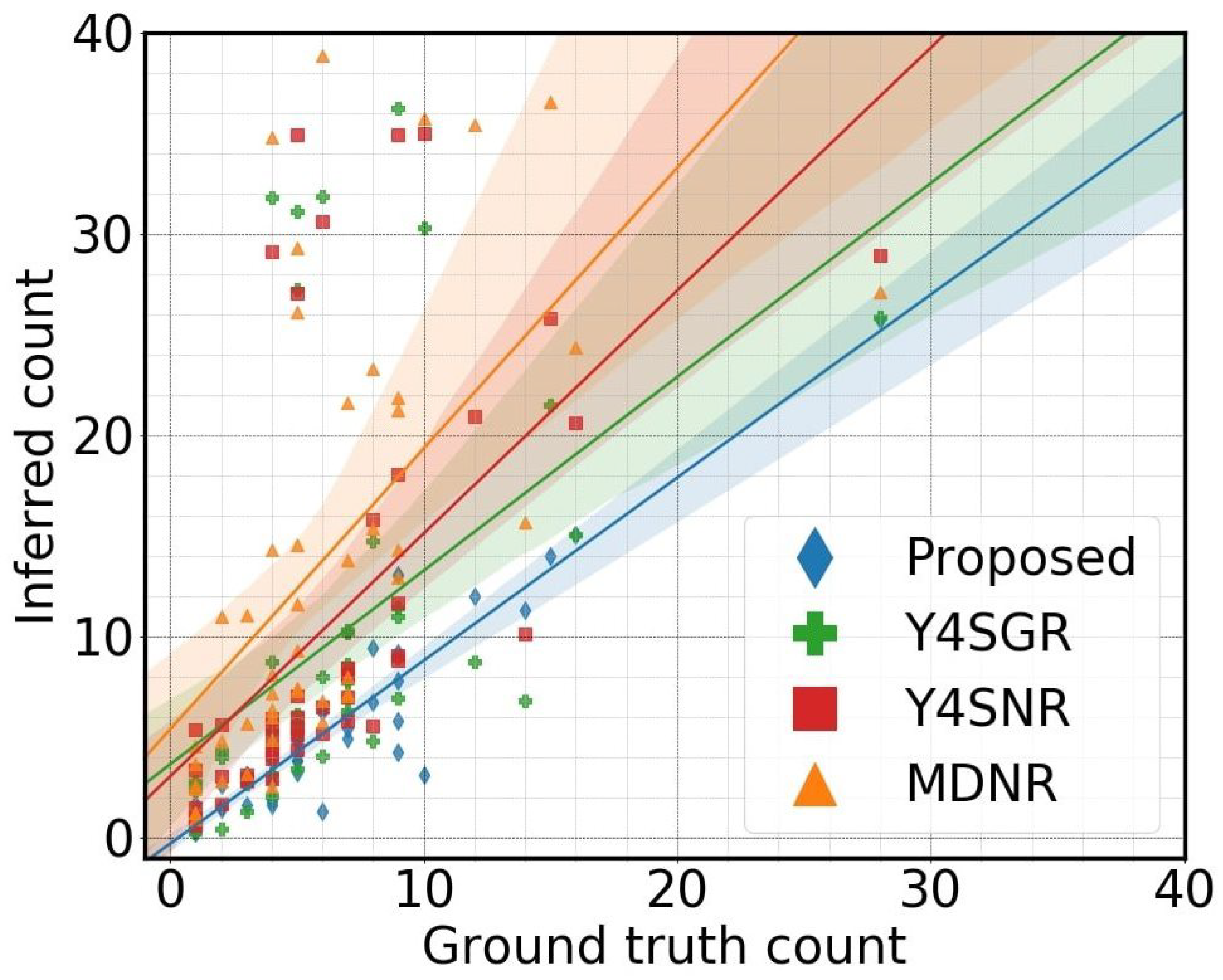
Figure 8 shows pairs of inferred counts plotted against ground-truth counts for each of the 55 road segment passes for select combinations of modules (including the best-performing one among all combinations) that reflect a wide range of performance. For a perfect automatic counting system, the scatter plot of inferred counts versus ground truth should be on the identity line (
y =
x). A regression line was estimated for each combination. The estimated lines are shown in
Figure 8, along with their confidence limits. Clearly, the proposed Y4SDR outperforms the other four combinations shown in
Figure 8 by a substantial margin.
As expected, the proposed homography-derived ROI performs better than the No ROI and the Generic ROI modules. The latter two ROI modules lead to over counts because of their limitations in distinguishing traffic participants from irrelevant vehicles. In contrast, the dynamic ROI allows for counting vehicles only in the pertinent parts of the road network, thus omitting irrelevant vehicles, which in this study consisted mostly of vehicles parked on the side of the roads or in adjacent parking lots. This result validates the developed bird’s-eye-view inverse projection approach to defining dynamic ROIs suitable to each roadway segment.
Figure 9 shows the eCDF plots of the four different functions from the four different trackers. In addition to confirming the overall superiority of the Y4SDR combination, these plots also indicate that this combination is highly reliable, as is evident from the thin tails of the distributions.
Summary results for all combinations of modules are shown in
Table 1. Specifically, the sample mean and sample median of absolute differences and absolute relative differences are given for each considered detector, tracker, and ROI combination. Across all combinations of detector and ROI options, SORT outperformed Deep SORT consistently. This result indicates that the deep association metric used by Deep SORT needs more training to be efficient. In addition, across all combinations of tracker and ROI options, the detectors Yolo v3 and Yolo v4 performed similarly and better than Mask-RCNN. This result indicates that two-stage detectors, such as Mask-RCNN, are prone to overfitting to the training data more than single-stage detectors. Moreover, it can be seen that for all detector and tracker combinations, the proposed dynamic ROI option outperforms the other two ROI options by a large margin, as one might expect. Finally, from the results in
Table 1, the Y4SDR combination is seen to perform the best among all combinations.
5.2. Impacts of Adverse Weather and Lighting
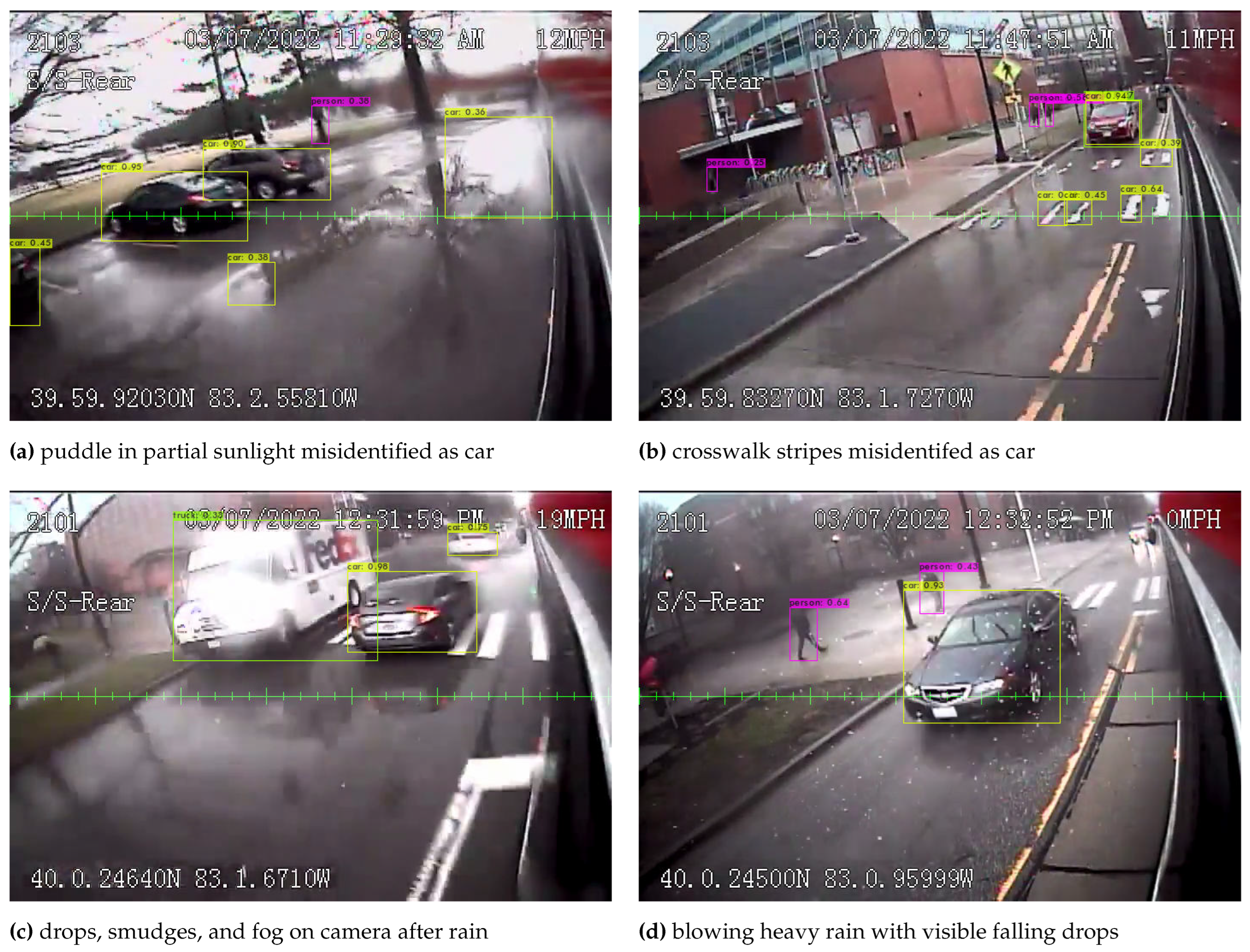
Having determined the best algorithm to implement from the results of the ablation study, one may also consider the performance of both the image processing and the overall counting system in the presence of inclement weather, including rain or post-rain conditions with puddles and irregular lighting effects. Inclement weather exposes several issues with an image-processing-based system, including darker and more varied lighting conditions, reflective puddles that can be misidentified as vehicles (
Figure 10a), roadway markings misidentified as vehicles (
Figure 10b), water droplets and smudges formed from dust or dirt and water partially obscuring some portions of the image (
Figure 10c), and finally, blowing heavy rain, or possibly snow, with falling drops that can be seen in the images (
Figure 10d).
We compared human-extracted ground truth with the automated extraction and counting results from videos of several loops of the West Campus route both on dry, cloudless, sunny days and days with rainfall varying from a light drizzle to heavy thunderstorms, which also included post-rain periods of time with breaking clouds that provided both darker and occasionally sunlit conditions. All the videos were acquired from actual in-service transit vehicles during the middle of the day.
Qualitatively, rainfall and wet conditions caused more transient—lasting only for one to two frames— inaccurate detection events to occur in the base image processing portion of the algorithm, including vehicles not detected, misclassified vehicles and other objects, and double detections when a vehicle is split into two overlapping objects, along with incorrectly identifying a greater number of background elements (e.g., puddles and road markings) as vehicles or objects. However, these transient events generally make little difference in the final vehicle counts, as the overall algorithm employs both filtering to eliminate unreasonable image processing results and tracking within the region of interest, such that a vehicle is declared present and counted only after a fairly complete track is established from the point it enters to the point it departs the camera’s field of view. This approach, in general terms, imposes continuity requirements, causing transient random events to be discarded unless they are so severe as to make it impossible to match and track a vehicle as it passes through the images, thereby improving the robustness of the approach.
More problematic, however, are persistent artifacts such as water droplets or smudges formed by wet dust and dirt, which often appear on the camera lens or enclosure cover after the rain stops and the lens begins to dry. For example, in one five-minute period of one loop, there was a large smudge on the left side at the vertical center of the lens, which obscured the region of the image where vehicles several lanes to the left of the transit bus tended to cross through and leave the image frame, causing them to not be counted due to incomplete tracking.
We note that these are general problems that can affect most video and image processing systems—if the lens is occluded you cannot see anything in that region of the image. It would be possible in future work to implement a method to dynamically detect when the lens is occluded and note the temporary exclusion of those regions from counts while the occlusion persists. As a final note, heavy rain was also observed to clean the lens.
Quantitatively, we present the results of the automated extraction and counting experiments in
Table 2 for both the dry, clear, sunny loops and the rainy and post-rain loops. The table presents the percentage of correctly counted vehicles, the percentage of vehicles missed due to not being detected at all or detected too infrequently to build a sufficient track, the percentage of vehicles not detected due to being substantially occluded by another vehicle (this is not actually a weather-related event but is included for completeness), and the percentage of vehicles not counted due to a smudge or water droplet covering part of the camera lens. The final columns of
Table 2 indicate the percentage of double-counted vehicles and the percentage of false detections or identifications that persisted long enough to be tracked and incorrectly counted. These are two impacts of transient image processing failures that are not always detected, at present, by our filtering and tracking algorithms.
As can be seen in
Table 2, the overall effects of poor weather conditions result in only a minor increase in the errors committed by this system.
6. Conclusions
This paper introduced and evaluated a fully automatic vision-based method for counting and tracking vehicles captured in video imagery from cameras mounted on buses for the purpose of estimating traffic flows on roadway segments using a previously developed moving observer methodology. The proposed method was implemented and tested using imagery from in-service transit buses, and its feasibility and accuracy was shown through experimental validation. Ablation studies were conducted to identify the best selection of alternative modules for the automated method.
The proposed method can be directly integrated into existing and future ground-vehicle-based traffic surveillance approaches. Furthermore, since cameras are ubiquitous, the proposed method can be utilized for different applications.
Reimagining public transit buses as data collection platforms has great promise. With widespread deployment of the previously developed moving observer methodology facilitated by the full automation of vehicle counting proposed in this paper, a new dimension can be added to intelligent traffic surveillance. Combined with more conventional methods, such as fixed location and the emerging possibilities of UAV-based surveillance, spatial and temporal coverage of roadway networks can be increased and made more comprehensive. This three-pronged approach has the potential of achieving close to full-coverage traffic surveillance in the future.
Future work could focus on further comprehensive evaluation of the method presented here under more varied conditions, subsequent refinements, and the use of edge computing technologies to perform the image processing and automatic counting onboard the buses in real time. Another potential extension would involve coordinated tracking of vehicles across multiple buses, although this raises certain social and political privacy issues that would need to be addressed. Finally, there could be significant uses and value in vehicle motion and classification information, potential extensions to include tracking and counting bicycles, motorcycles, and pedestrians, and the eventual integration into smart city infrastructure deployments.


 ,
, 


