
Rapid Post-Earthquake Structural Damage Assessment Using Convolutional Neural Networks and Transfer Learning


Abstract
:1. Introduction
2. Related Studies
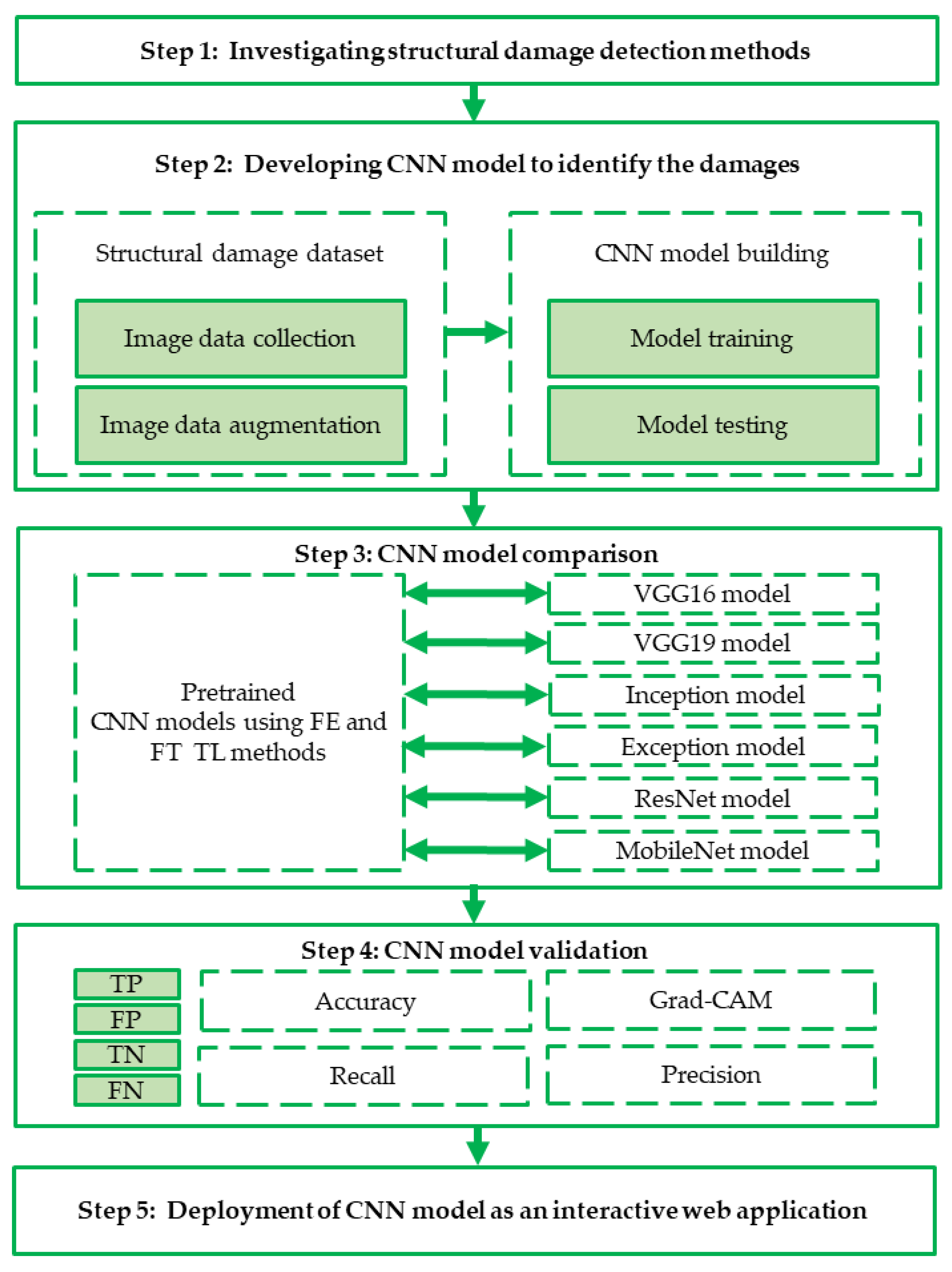
3. Methodology
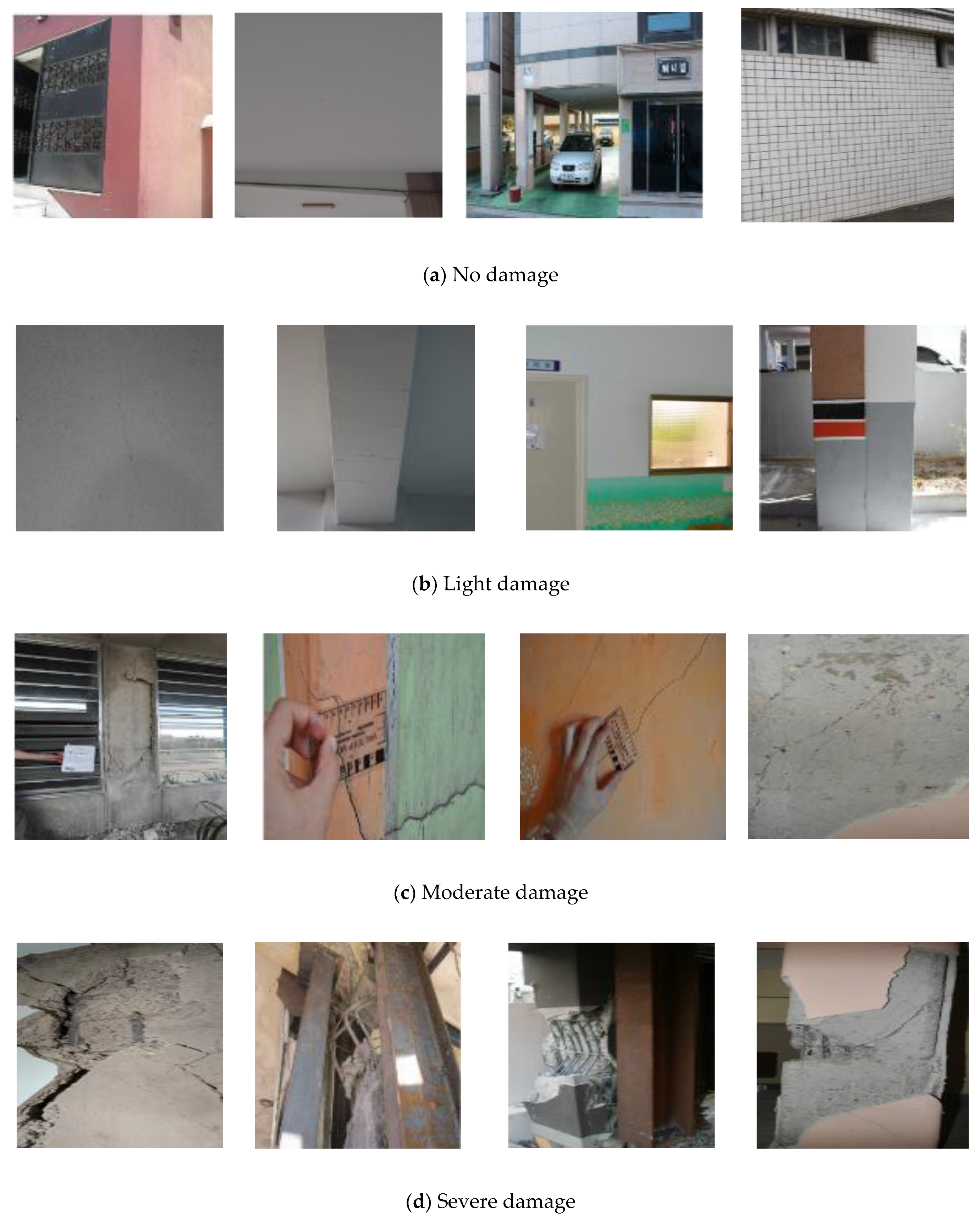
3.1. Data Acquisition, Division, and Preprocessing
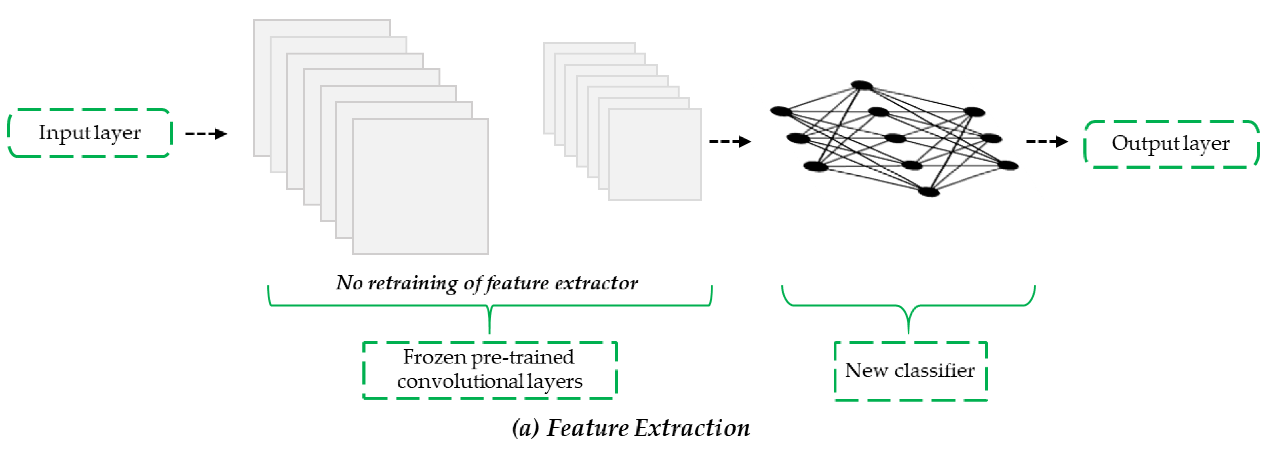
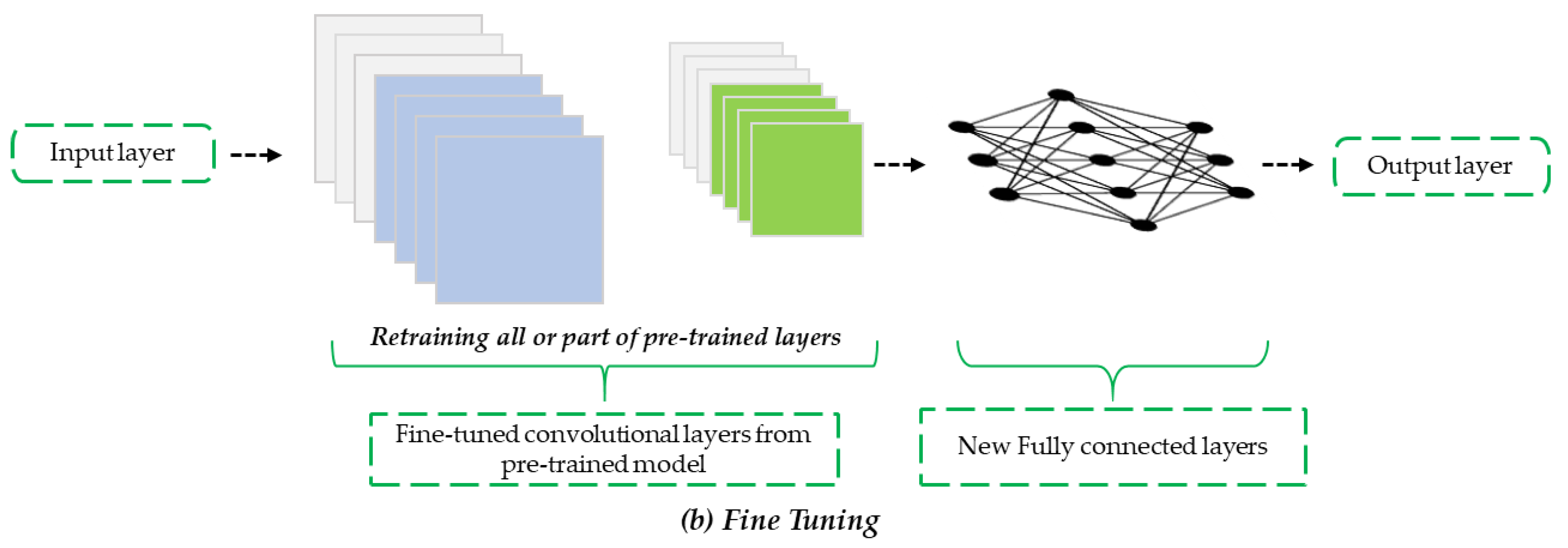
3.2. TL Using Pre-Trained CNN Models
4. Results and Discussion
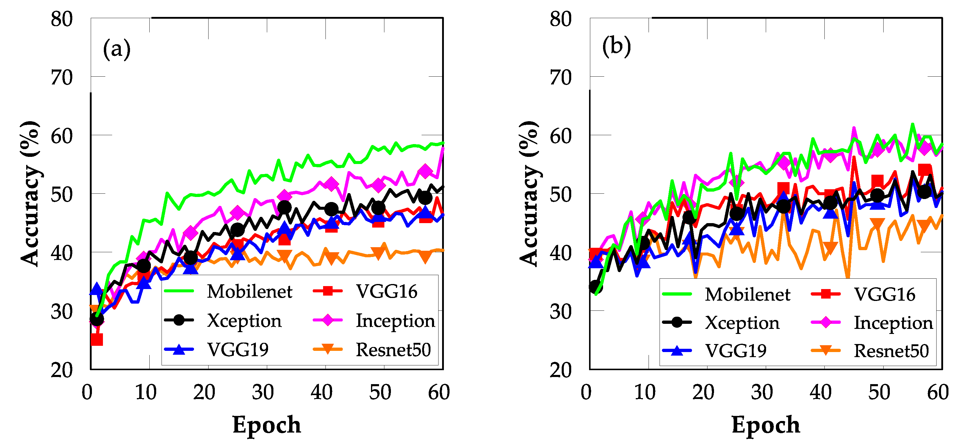
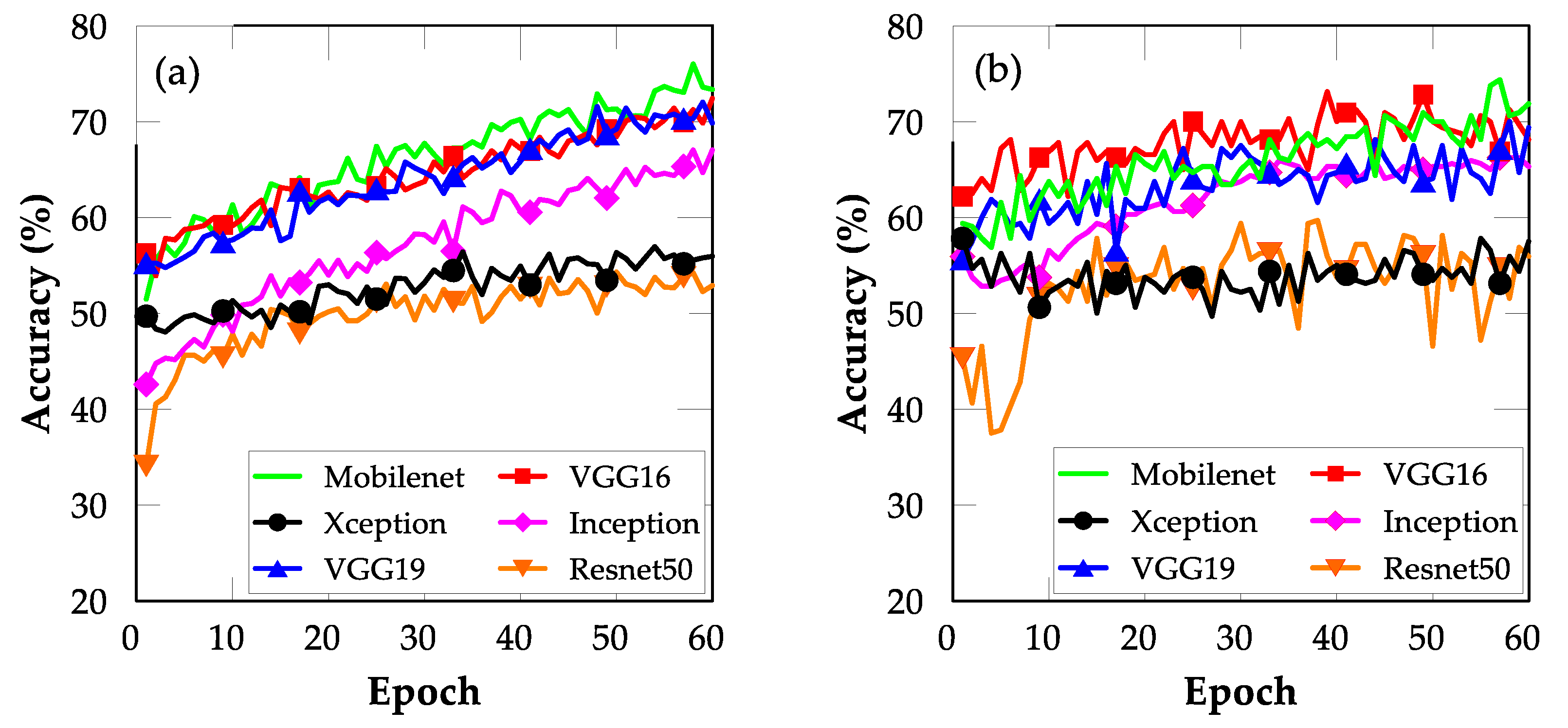
4.1. FE with Bottleneck Features
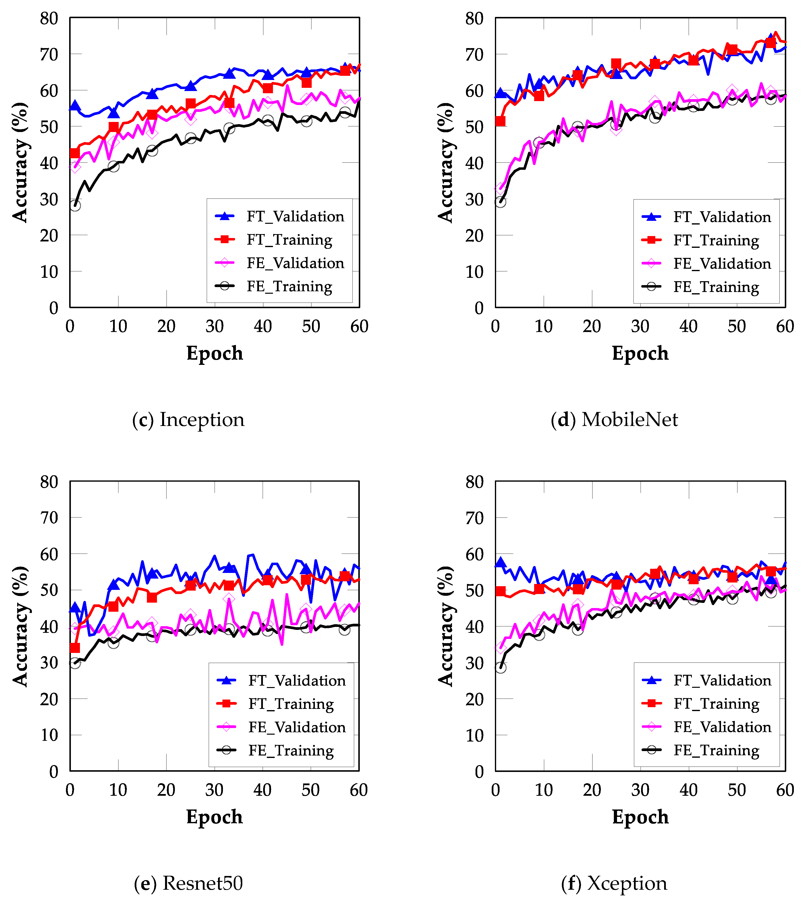
4.2. FT
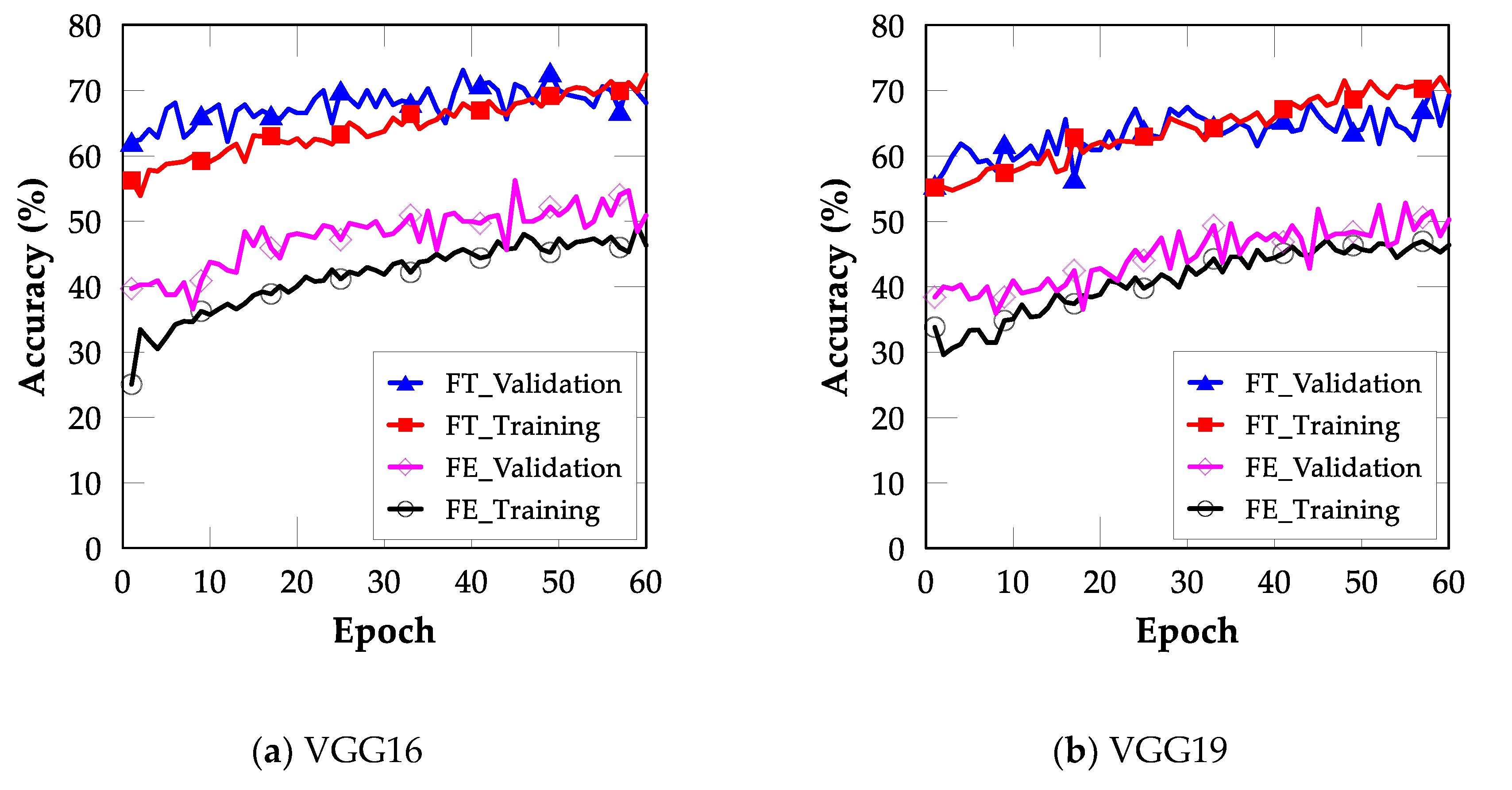
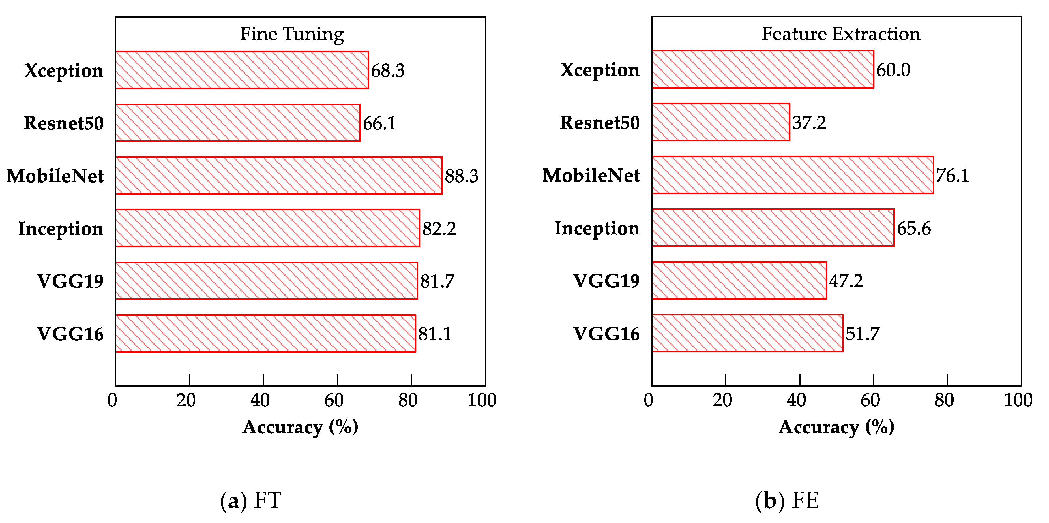
4.3. Comparison between FE and FT
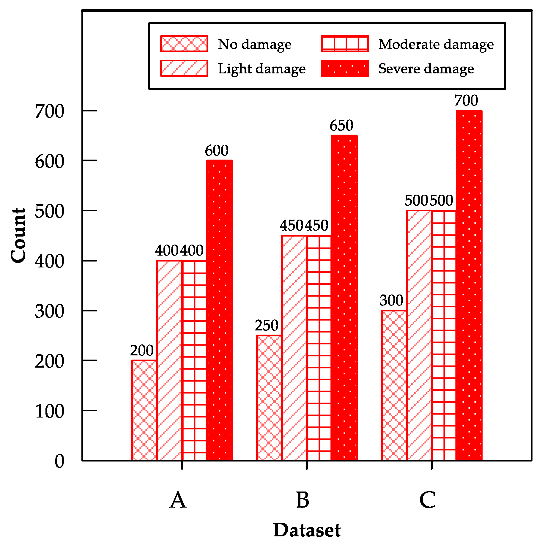
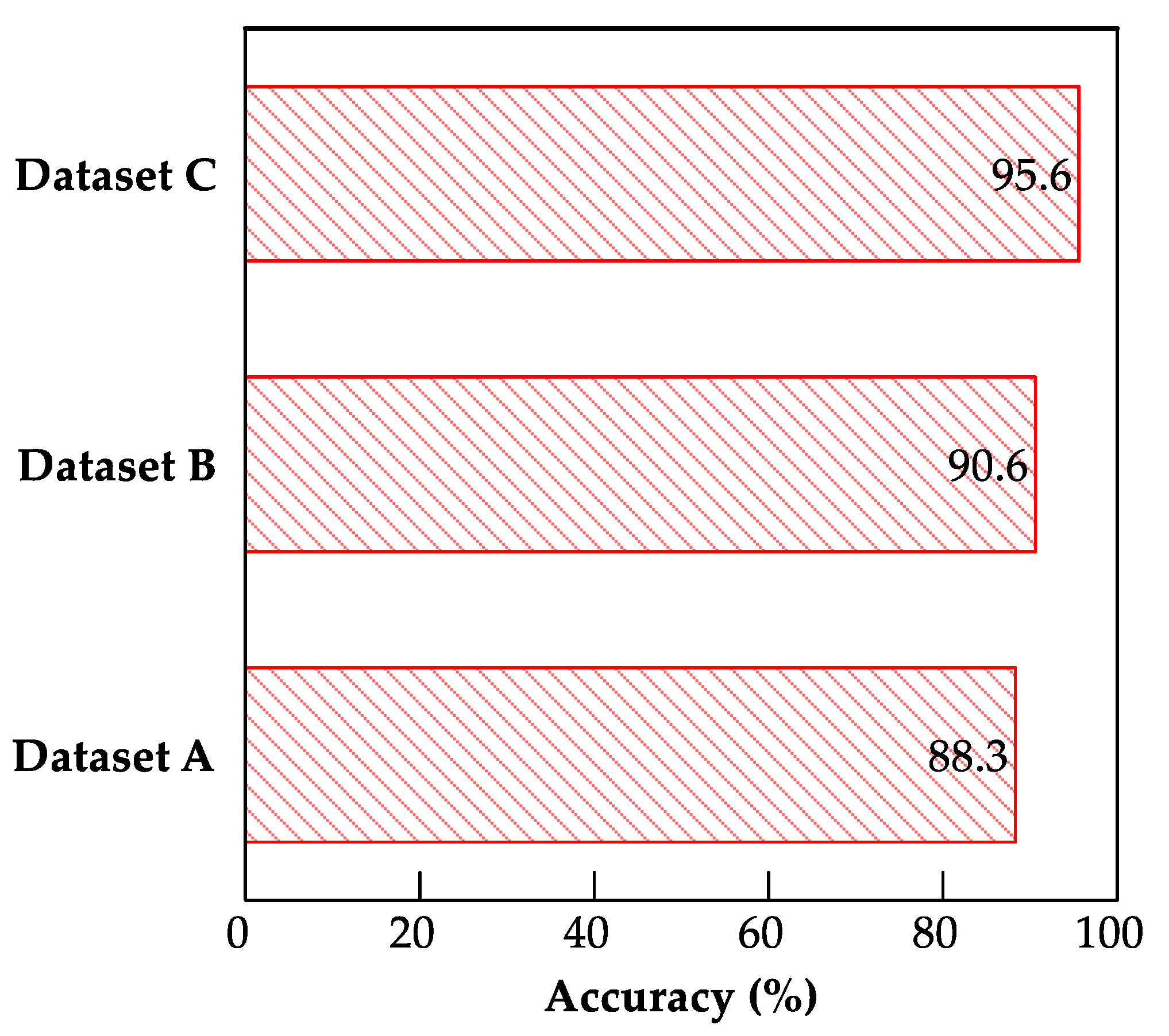
4.4. Comparative Study: Effect of Dataset Size on Fine-Tuned Model
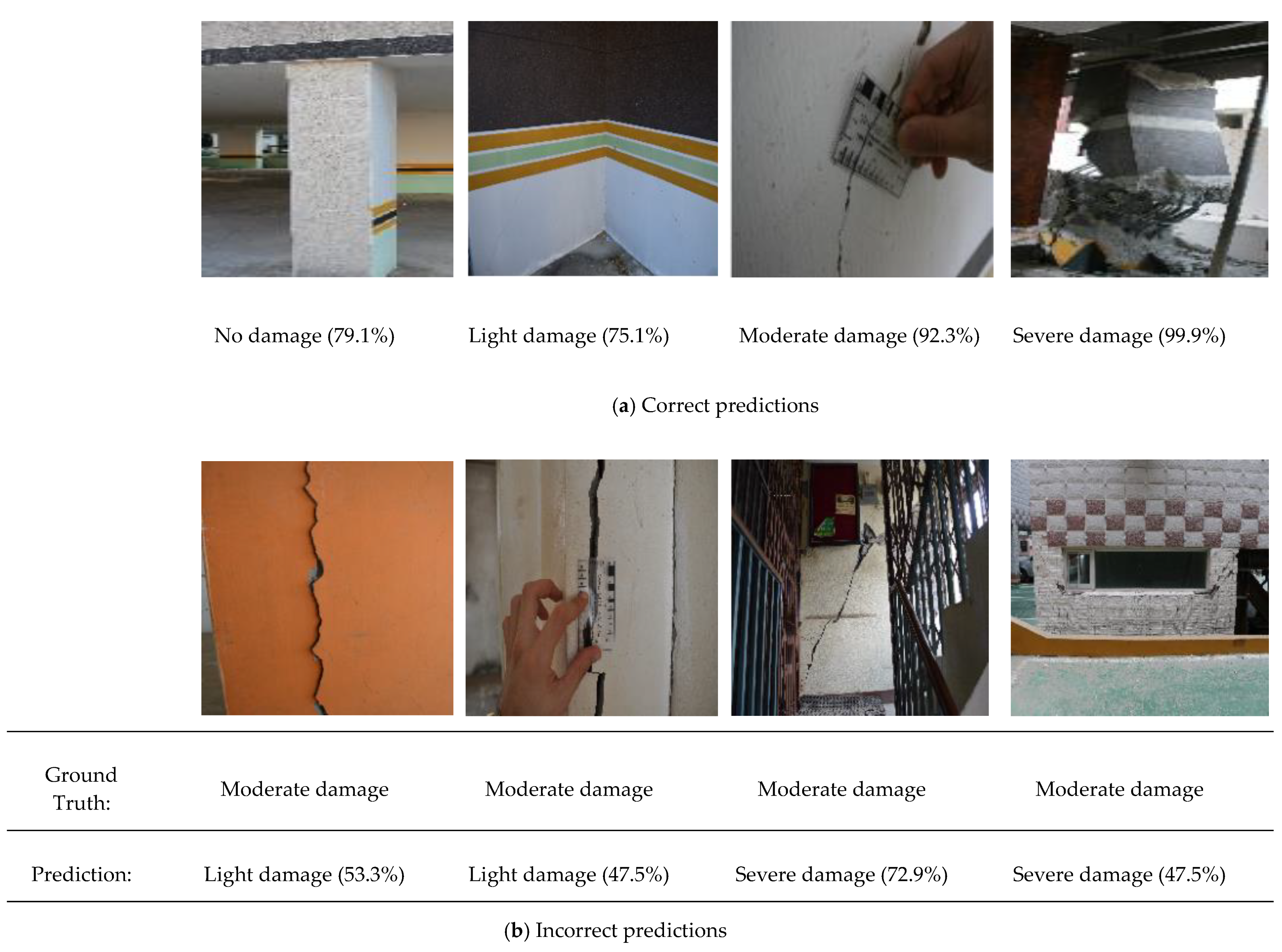
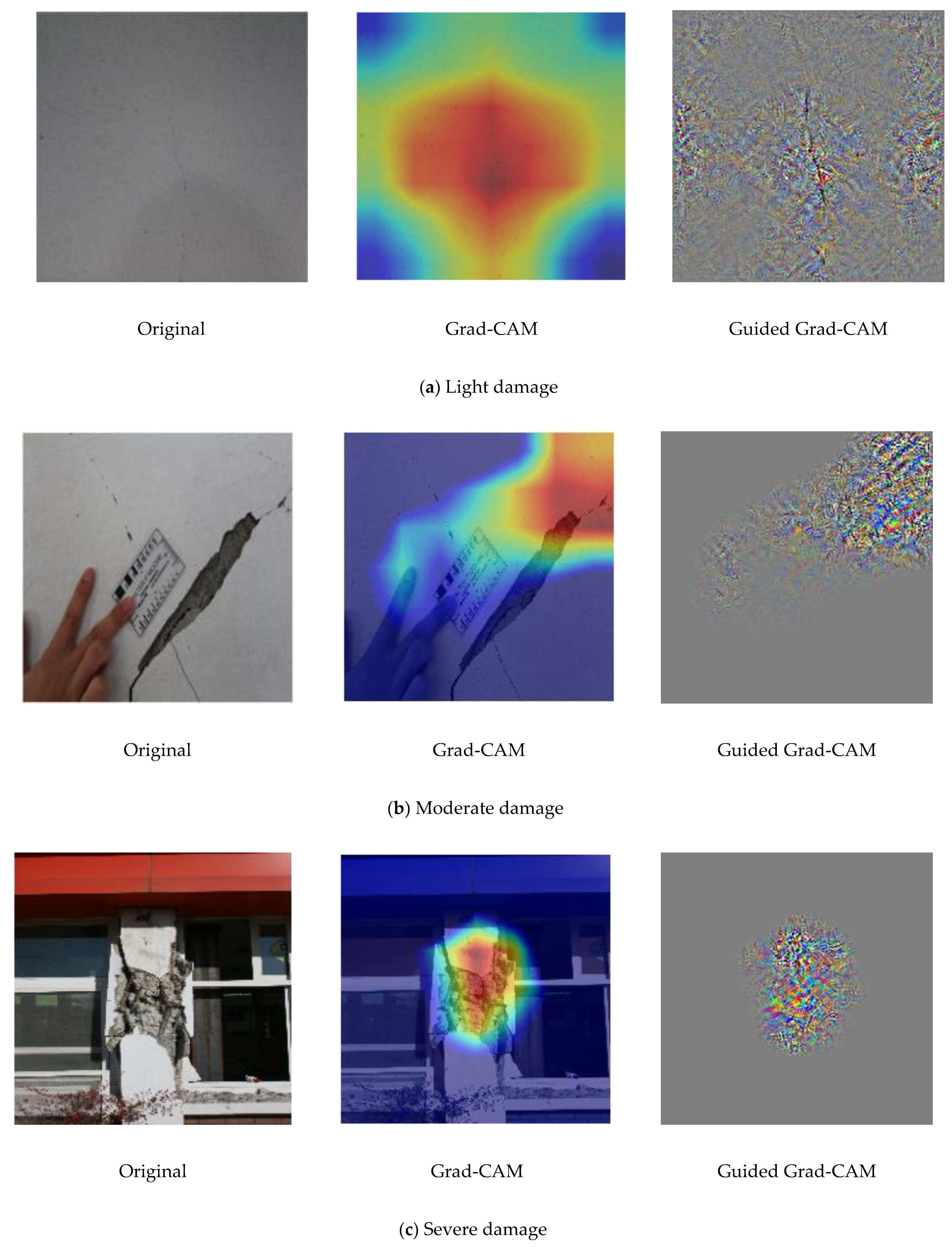
4.5. Visualization and Localization of Damage Using Grad-CAM
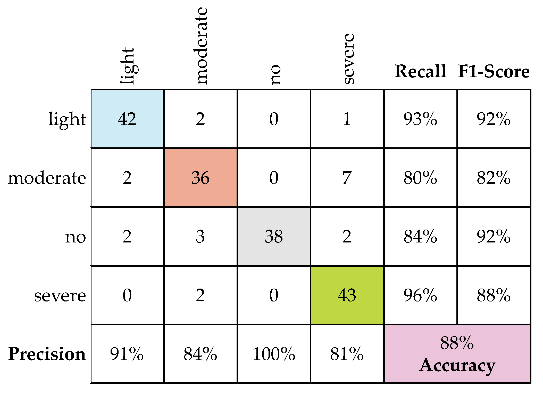
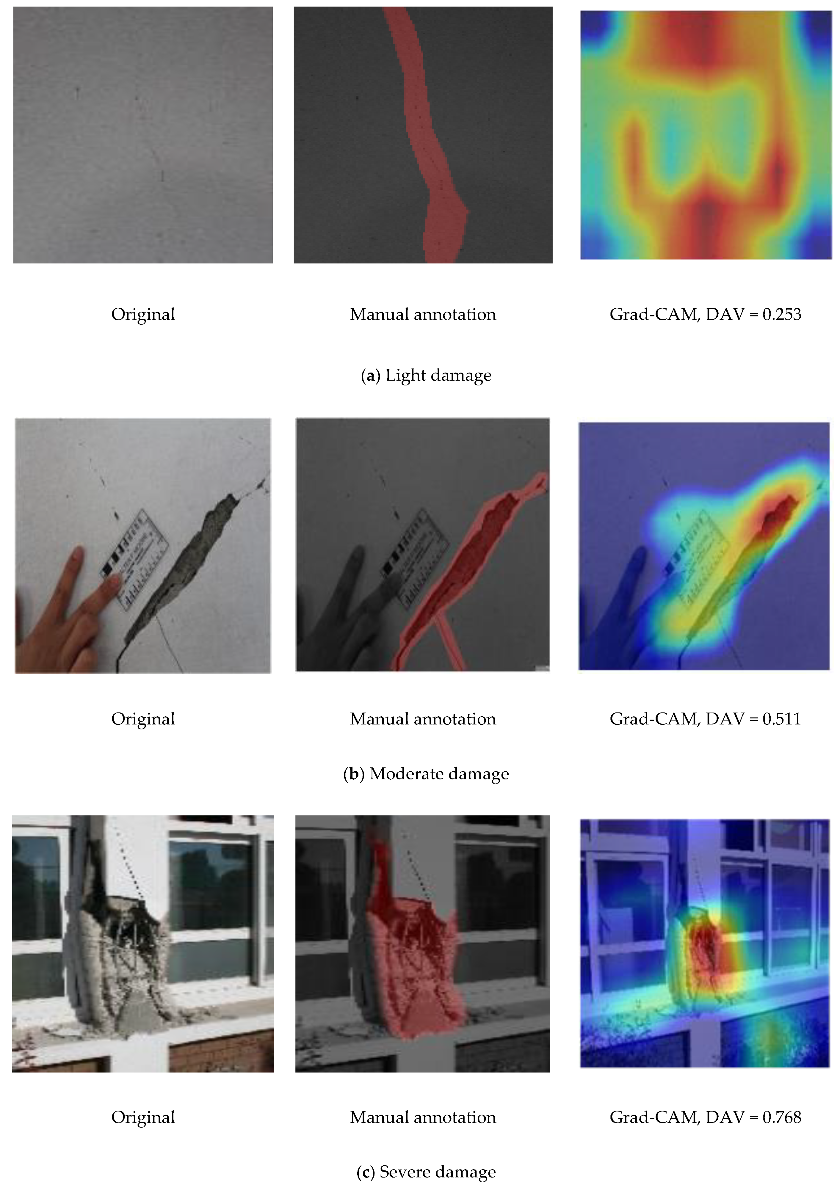
4.6. Damage Severity Measurement
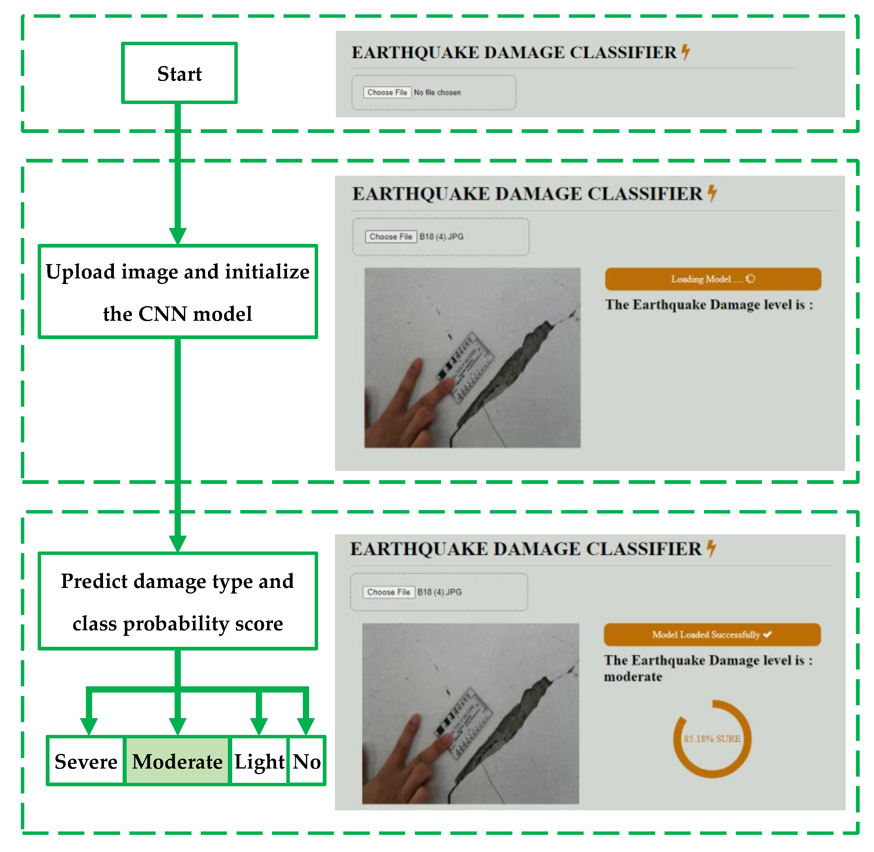
5. Development of CNN Model as Interactive Web Application
6. Conclusions and Recommendations
- The FT method outperformed the FE method for all the CNN models evaluated. However, the FT method is more computationally complex than the FE method because it involves retraining one convolutional block.
- The MobileNet model exhibited the best performance for both the FE and FT TL methods, exhibiting testing accuracies of 76.1% and 88.3%, respectively. The superiority of the MobileNet model in performing classification promoted its deployment as a web-based application for earthquake-damage classification.
- The web application successfully predicted the damage class in new images of seismic damage with high certainty. In addition, interactive web pages can rapidly and automatically classify SD from earthquakes, thereby facilitating decision making in response to earthquakes.
Author Contributions
Funding
Conflicts of Interest
Abbreviations
| CNN | Convolutional neural network |
| DAV | Damage assessment value |
| DDM | Damage detection map |
| DL | Deep learning |
| FE | Feature extraction |
| FT | Fine-tuning |
| GPU | Graphic processing unit |
| Grad-CAM | Gradient-weighted class activation mapping |
| OLeNet | Optimized LeNet |
| PEER | Pacific Earthquake Engineering Research |
| ReLU | Rectified linear unit |
| SD | Structural damage |
| TL | Transfer learning |
| VGG | Visual geometry group |
References
- Lowes, L.; DesRoches, R.; Eberhard, M.; Parra-Montesinos, G. NSF RAPID: Collection of Damage Data Following Haiti Earthquake (NEES-2010-0872) 2017. Available online: https://datacenterhub.org/resources/14372 (accessed on 21 August 2020).
- NCREE; Purdue University. Performance of Reinforced Concrete Buildings in the 2016 Taiwan (Meinong) Earthquake 2016. Available online: https://datacenterhub.org/resources/14098 (accessed on 21 August 2020).
- Shah, P.; Pujol, S.; Puranam, A.; Laughery, L. Database on Performance of Low-Rise Reinforced Concrete Buildings in the 2015 Nepal Earthquake; Purdue University Research Repository: Lafayette, IN, USA, 2015; Available online: https://datacenterhub.org/resources/238 (accessed on 21 August 2020).
- Sim, C.; Laughery, L.; Chiou, T.C.; Weng, P. 2017 Pohang Earthquake-Reinforced Concrete Building Damage Survey. 2018. Available online: https://datacenterhub.org/resources/14728 (accessed on 21 August 2020).
- Sim, C.; Villalobos, E.; Smith, J.P.; Rojas, P.; Pujol, S.; Puranam, A.Y.; Laughery, L. Performance of Low-Rise Reinforced Concrete Buildings in the 2016 Ecuador Earthquake. 2016. Available online: https://datacenterhub.org/resources/14160 (accessed on 21 August 2020).
- Gao, Y.; Mosalam, K.M. Deep transfer learning for image-based structural damage recognition. Comput. Aid. Civ. Infrastruct. Eng. 2018, 33, 748–768. [Google Scholar] [CrossRef]
- Nahata, D.; Mulchandani, H.; Bansal, S.; Muthukumar, G. Post-earthquake assessment of buildings using deep learning. arXiv 2019, arXiv:1907.07877. [Google Scholar]
- Pan, X.; Yang, T.Y. Postdisaster image-based damage detection and repair cost estimation of reinforced concrete buildings using dual convolutional neural networks. Comput. Aided Civ. Infrastruct. Eng. 2020, 35, 495–510. [Google Scholar] [CrossRef]
- Hoskere, V.; Narazaki, Y.; Hoang, T.A.; Spencer, B.F., Jr. Vision-based structural inspection using multiscale deep convolutional neural networks. In Proceedings of the 3rd Huixian International Forum on Earthquake Engineering for Young Researchers, Urbana-Champaign, IL, USA, 11–12 August 2012. [Google Scholar]
- Zhai, W.; Peng, Z.R. Damage assessment using Google street view: Evidence from hurricane Michael in Mexico Beach, Florida. Appl. Geogr. 2020, 123, 102252. [Google Scholar] [CrossRef]
- Liang, X. Image-based post-disaster inspection of reinforced concrete bridge systems using deep learning with Bayesian optimization. Comput. Aided Civ. Infrastruct. Eng. 2019, 34, 415–430. [Google Scholar] [CrossRef]
- Gao, Y.; Mosalam, K.M. PEER Hub ImageNet (Ø-Net): A Large-Scale Multi-Attribute Benchmark Dataset of Structural Images; Report No. 2019/07; Earthquake Engineering Research Center Headquarters at the University of California: Berkeley, CA, USA, 2019. [Google Scholar] [CrossRef]
- Naser, M.Z.; Kodur, V.; Thai, H.T.; Hawileh, R.; Abdalla, J.; Degtyarev, V.V. StructuresNet and FireNet: Benchmarking databases and machine learning algorithms in structural and fire engineering domains. J. Build. Eng. 2021, 44, 102977. [Google Scholar] [CrossRef]
- Cha, Y.J.; Choi, W.; Büyüköztürk, O. Deep learning-based crack damage detection using convolutional neural networks. Comput. Aided Civ. Infrastruct. Eng. 2017, 32, 361–378. [Google Scholar] [CrossRef]
- Ghosh Mondal, T.G.; Jahanshahi, M.R.; Wu, R.T.; Wu, Z.Y. Deep learning-based multi-class damage detection for autonomous post-disaster reconnaissance. Str. Control Health Monit. 2020, 27, e2507. [Google Scholar] [CrossRef]
- Li, X.; Caragea, D.; Zhang, H.; Imran, M. Localizing and quantifying infrastructure damage using class activation mapping approaches. Soc. Netw. Anal. Min. 2019, 9, 44. [Google Scholar] [CrossRef]
- Kim, B.; Yuvaraj, N.; Park, H.W.; Preethaa, K.R.S.; Pandian, R.A.; Lee, D. Investigation of steel frame damage based on computer vision and deep learning. Autom. Constr. 2021, 132, 103941. [Google Scholar] [CrossRef]
- Spencer, B.F.; Hoskere, V.; Narazaki, Y. Advances in computer vision-based civil infrastructure inspection and monitoring. Engineering 2019, 5, 199–222. [Google Scholar] [CrossRef]
- Sony, S.; Dunphy, K.; Sadhu, A.; Capretz, M. A Systematic Review of Convolutional Neural Network-Based Structural Condition Assessment Techniques. Eng. Struct. 2021, 226, 111347. [Google Scholar] [CrossRef]
- Kim, B.; Serfa Juan, R.O.S.; Lee, D.-E.; Chen, Z. Importance of image enhancement and CDF for fault assessment of photovoltaic module using IR thermal image. Appl. Sci. 2021, 11, 8388. [Google Scholar] [CrossRef]
- Kim, B.; Yuvaraj, N.; Sri Preethaa, K.R.; Santhosh, R.; Sabari, A. Enhanced pedestrian detection using optimized deep convolution neural network for smart building surveillance. Soft Comput. 2020, 24, 17081–17092. [Google Scholar] [CrossRef]
- Kim, B.; Yuvaraj, N.; Sri Preethaa, K.R.; Arun Pandian, R. Surface crack detection using deep learning with shallow CNN architecture for enhanced computation. Neural Comput. Appl. 2021, 33, 9289–9305. [Google Scholar] [CrossRef]
- ATC-58. Development of next Generation Performance-Based Seismic Design Procedures for New and Existing Buildings. ATC 2007. Redwood City, CA, USA. Available online: https://www.atcouncil.org (accessed on 28 March 2022).
- Yuvaraj, N.; Kim, B.; Preethaa, K.R.S. Transfer learning based real-time crack detection using unmanned aerial system. Int. J. High-Rise Build. 2020, 9, 351–360. [Google Scholar] [CrossRef]
- Dhanamjayulu, C.; Nizhal, U.N.; Maddikunta, P.K.R.; Gadekallu, T.R.; Iwendi, C.; Wei, C.; Xin, Q. Identification of malnutrition and prediction of BMI from facial images using real-time image processing and machine learning. IET Image Process. 2022, 16, 647–658. [Google Scholar] [CrossRef]
- Perez, H.; Tah, J.H.M.; Mosavi, A. Deep learning for detecting building defects using convolutional neural networks. Sensors 2019, 19, 3556. [Google Scholar] [CrossRef] [Green Version]
- Zhang, C.; Chang, C.-C.; Jamshidi, M. Concrete bridge surface damage detection using a single-stage detector. Comput. Aided Civ. Infrastruct. Eng. 2020, 35, 389–409. [Google Scholar] [CrossRef]
- Dais, D.; Bal, İ.E.; Smyrou, E.; Sarhosis, V. Automatic crack classification and segmentation on masonry surfaces using convolutional neural networks and transfer learning. Autom. Constr. 2021, 125, 103606. [Google Scholar] [CrossRef]
- Dung, C.V.; Anh, L.D. Autonomous concrete crack detection using deep fully convolutional neural network. Autom. Constr. 2019, 99, 52–58. [Google Scholar] [CrossRef]
- Zhang, Y.; Sun, X.; Loh, K.J.; Su, W.; Xue, Z.; Zhao, X. Autonomous bolt loosening detection using deep learning. Str. Health Monit. 2019, 19, 105–122. [Google Scholar] [CrossRef]
- Liu, H.; Zhang, Y. Image-driven structural steel damage condition assessment method using deep learning algorithm. Measurement 2019, 133, 168–181. [Google Scholar] [CrossRef]
- Ali, L.; Alnajjar, F.; Jassmi, H.A.; Gocho, M.; Khan, W.; Serhani, M.A. Performance evaluation of deep CNN-based crack detection and localization techniques for concrete structures. Sensors 2021, 21, 1688. [Google Scholar] [CrossRef] [PubMed]
- Chen, J.; Yang, T.; Zhang, D.; Huang, H.; Tian, Y. Deep learning based classification of rock structure of tunnel face. Geosci. Front. 2021, 12, 395–404. [Google Scholar] [CrossRef]
- Harvey, W.; Rainwater, C.; Cothren, J. Direct aerial visual geolocalization using deep neural networks. Remote Sens. 2021, 13, 4017. [Google Scholar] [CrossRef]
- Nath, N.D.; Behzadan, A.H.; Paal, S.G. Deep learning for site safety: Real-time detection of personal protective equipment. Autom. Constr. 2020, 112, 103085. [Google Scholar] [CrossRef]
- Narazaki, Y.; Hoskere, V.; Hoang, T.A.; Fujino, Y.; Sakurai, A.; Spencer, B.F. Vision-based automated bridge component recognition with high-level scene consistency. Comput. Aided Civ. Infrastruct. Eng. 2020, 35, 465–482. [Google Scholar] [CrossRef]
- Bang, S.; Park, S.; Kim, H.; Kim, H. Encoder–decoder network for pixel-level road crack detection in black-box images. Comput. Aided Civ. Infrastruct. Eng. 2019, 34, 713–727. [Google Scholar] [CrossRef]
- Maeda, H.; Sekimoto, Y.; Seto, T.; Kashiyama, T.; Omata, H. Road damage detection and classification using deep neural networks with smartphone images. Comput. Aided Civ. Infrastruct. Eng. 2018, 33, 1127–1141. [Google Scholar] [CrossRef]
- Cheng, C.S.; Behzadan, A.H.; Noshadravan, A. Deep learning for post-hurricane aerial damage assessment of buildings. Comput. Aided Civ. Infrastruct. Eng. 2021, 36, 695–710. [Google Scholar] [CrossRef]
- Selvaraju, R.R.; Cogswell, M.; Das, A.; Vedantam, R.; Parikh, D.; Batra, D. Grad-CAM: Visual explanations from deep networks via gradient-based localization. Int. J. Comput. Vis. 2020, 128, 336–359. [Google Scholar] [CrossRef] [Green Version]
- Russell, B.C.; Torralba, A.; Murphy, K.P.; Freeman, W.T. LabelMe: A database and web-based tool for image annotation. Int. J. Comput. Vis. 2008, 77, 157–173. [Google Scholar] [CrossRef]
- Nia, K.R.; Mori, G. Building Damage Assessment Using Deep Learning and Ground-Level Image Data. In Proceedings of the 14th Conference on Computer and Robot Vision (CRV), Edmonton, AB, Canada, 16–19 May 2017; IEEE Publications: Piscataway, NJ, USA, 2017; Volume 2017, pp. 95–102. [Google Scholar] [CrossRef]
- TensorFlow. Js. Available online: https://www.tensorflow.org/js (accessed on 22 February 2022).


| Image Source | No Damage | Light Damage | Moderate Damage | Severe Damage |
|---|---|---|---|---|
| Pohang (2017) [4] | 49 | 294 | 187 | 551 |
| Haiti (2010) [1] | 52 | 55 | 174 | 127 |
| Nepal (2015) [3] | 152 | 153 | 123 | 255 |
| Taiwan (2016) [2] | 3 | 99 | 27 | 34 |
| Ecuador (2016) [5] | 4 | 108 | 115 | 188 |
| Total | 260 | 709 | 626 | 1155 |
| Image | No Damage | Light Damage | Moderate Damage | Severe Damage |
|---|---|---|---|---|
| Training | 160 | 320 | 320 | 480 |
| Validation | 40 | 80 | 80 | 120 |
| Testing | 45 | 45 | 45 | 45 |
| Total | 245 | 445 | 445 | 645 |
| CNN Algorithm |
|---|
| Programming language used for implementation: Python. Libraries for CNN model building: Tensorflow and Keras. Libraries used for image augmentation: OpenCV and computer vision library. Libraries used for visualizations: Matplotlib and 2D graph tool.
|
| Model | No. of Parameters | Depth of Layers | Size (MB) |
|---|---|---|---|
| VGG16 | 138.4 M | 16 | 528 |
| VGG19 | 143.7 M | 19 | 549 |
| Inception | 23.9 M | 189 | 92 |
| Xception | 22.9 M | 81 | 88 |
| ResNet | 25.6 M | 107 | 98 |
| MobileNet | 4.3 M | 55 | 16 |
| Task Description | Algorithm | Accuracy (%) | * Precision (%) | * Recall (%) | References |
|---|---|---|---|---|---|
| Classification of damage in all structural members | VGG16 | 68.8 | - | - | [6] |
| Classification of damage in columns only | ResNet50 | 87.47 | - | - | [8] |
| Classification of damage in all structural members | MobileNet | 88.3 | 89 | 88.2 | Current work |
Publisher’s Note: MDPI stays neutral with regard to jurisdictional claims in published maps and institutional affiliations. |
© 2022 by the authors. Licensee MDPI, Basel, Switzerland. This article is an open access article distributed under the terms and conditions of the Creative Commons Attribution (CC BY) license (https://creativecommons.org/licenses/by/4.0/).
Share and Cite
Ogunjinmi, P.D.; Park, S.-S.; Kim, B.; Lee, D.-E. Rapid Post-Earthquake Structural Damage Assessment Using Convolutional Neural Networks and Transfer Learning. Sensors 2022, 22, 3471. https://doi.org/10.3390/s22093471
Ogunjinmi PD, Park S-S, Kim B, Lee D-E. Rapid Post-Earthquake Structural Damage Assessment Using Convolutional Neural Networks and Transfer Learning. Sensors. 2022; 22(9):3471. https://doi.org/10.3390/s22093471
Chicago/Turabian StyleOgunjinmi, Peter Damilola, Sung-Sik Park, Bubryur Kim, and Dong-Eun Lee. 2022. "Rapid Post-Earthquake Structural Damage Assessment Using Convolutional Neural Networks and Transfer Learning" Sensors 22, no. 9: 3471. https://doi.org/10.3390/s22093471
APA StyleOgunjinmi, P. D., Park, S.-S., Kim, B., & Lee, D.-E. (2022). Rapid Post-Earthquake Structural Damage Assessment Using Convolutional Neural Networks and Transfer Learning. Sensors, 22(9), 3471. https://doi.org/10.3390/s22093471