
Adversarial Resolution Enhancement for Electrical Capacitance Tomography Image Reconstruction


Abstract
:1. Introduction
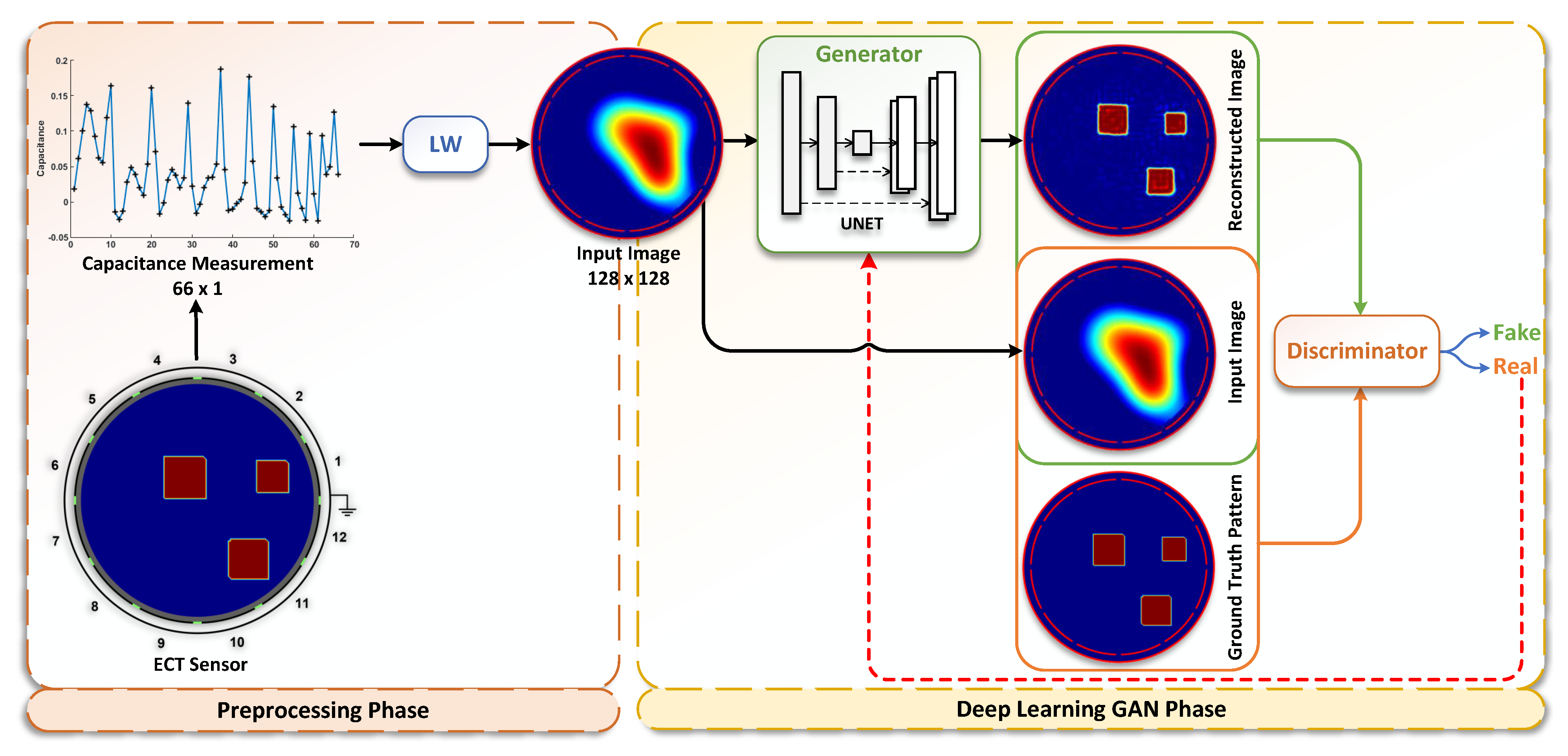
- The adversarial resolution enhancement (ARE-ECT) model was developed in the problem of the ECT image reconstruction quality improvement.
- The proposed model aimed to predict enhanced ECT image reconstructions from the lower quality ones.
- Our CGAN-based approach produces qualitative and quantitative improved results in ECT image resolution better than current complex and time-consuming non-linear reconstruction algorithms.
2. Problem Statement
3. Deep Neural Network Models
3.1. GAN
3.2. CGAN
4. ARE-ECT Model
5. ECT Dataset
6. Experimental Results and Analysis
6.1. Validation Metrics
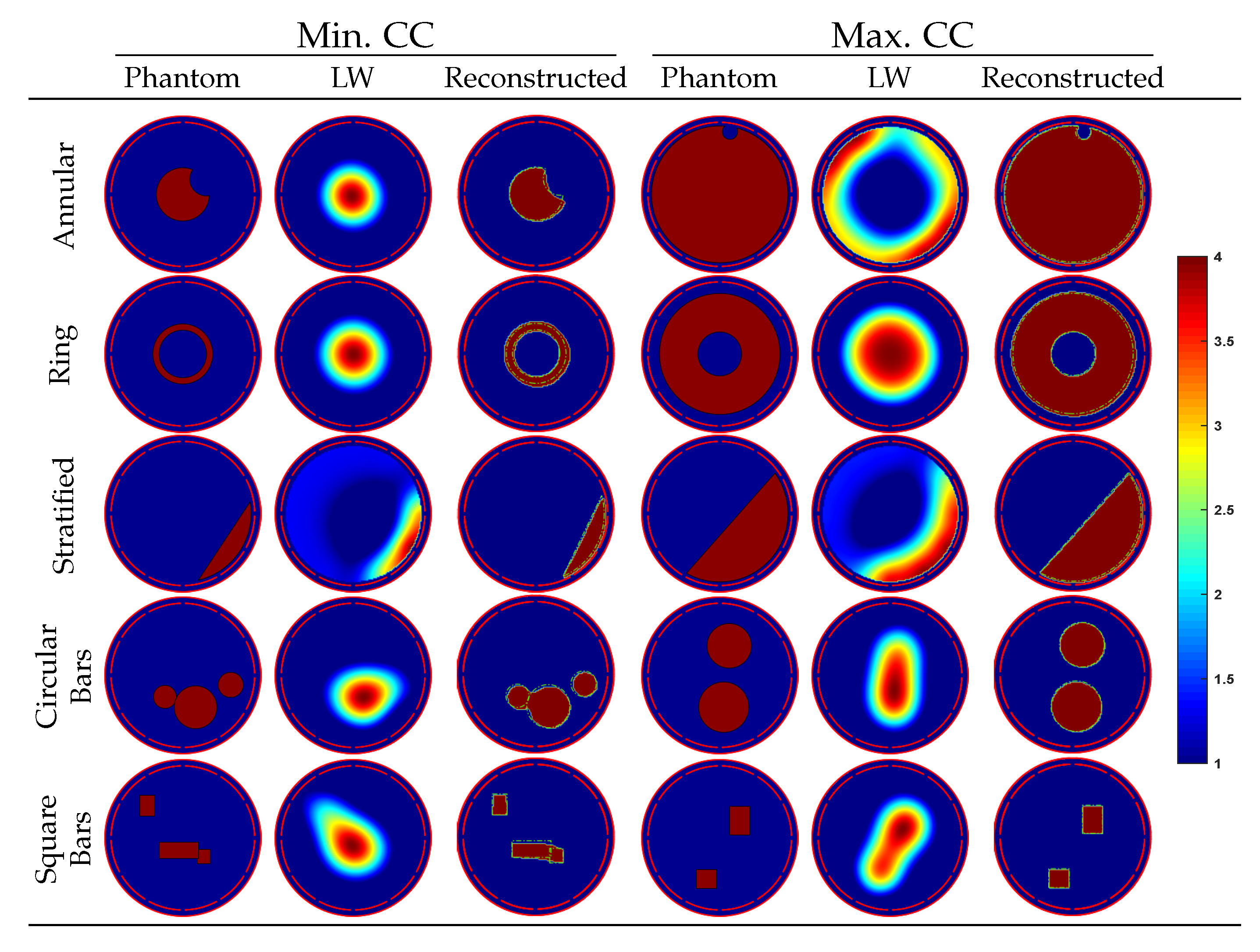
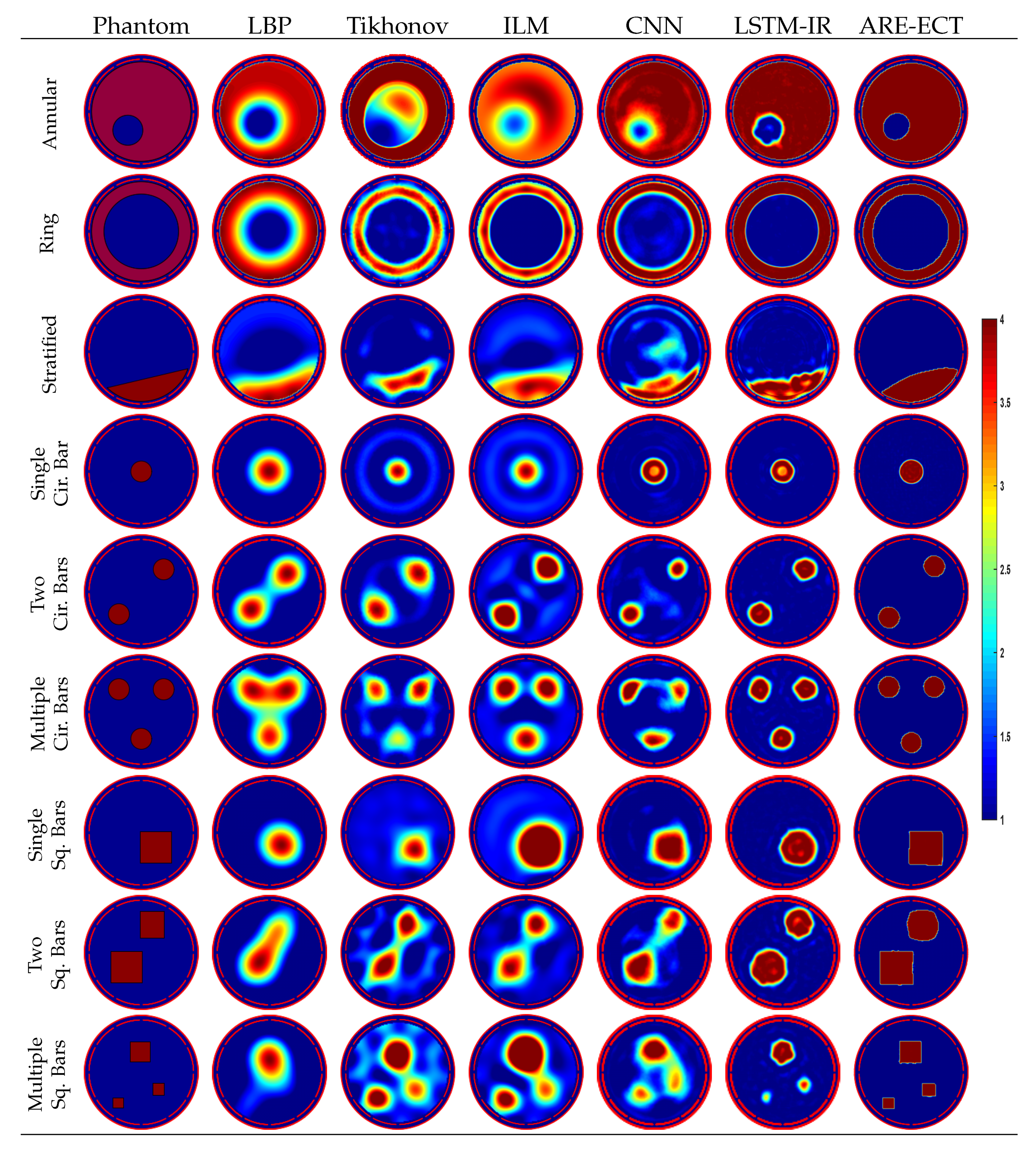
6.2. Qualitative Results on Simulation Test Dataset
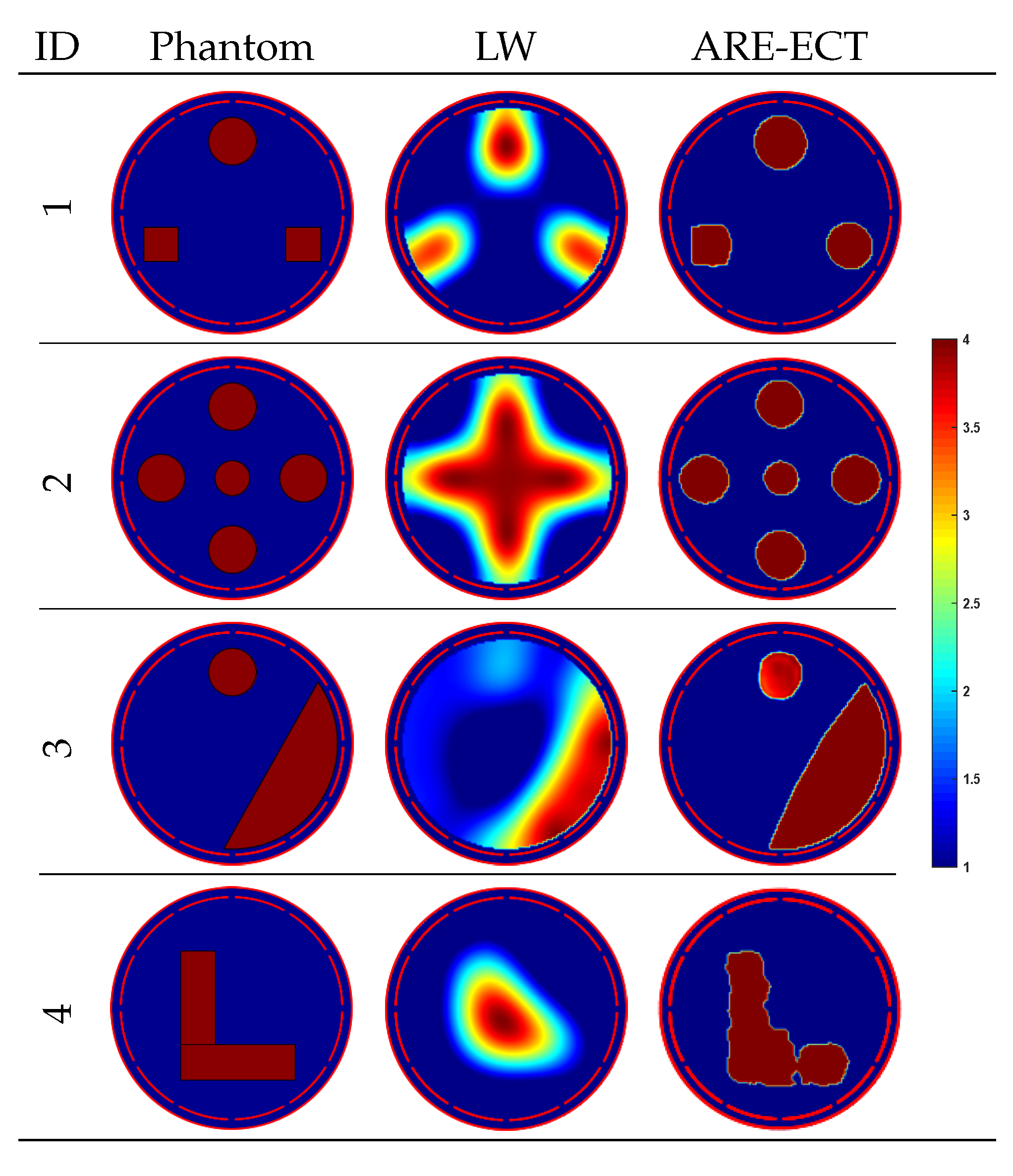
6.3. Testing Results of Non-Existing Phantoms in Training Dataset
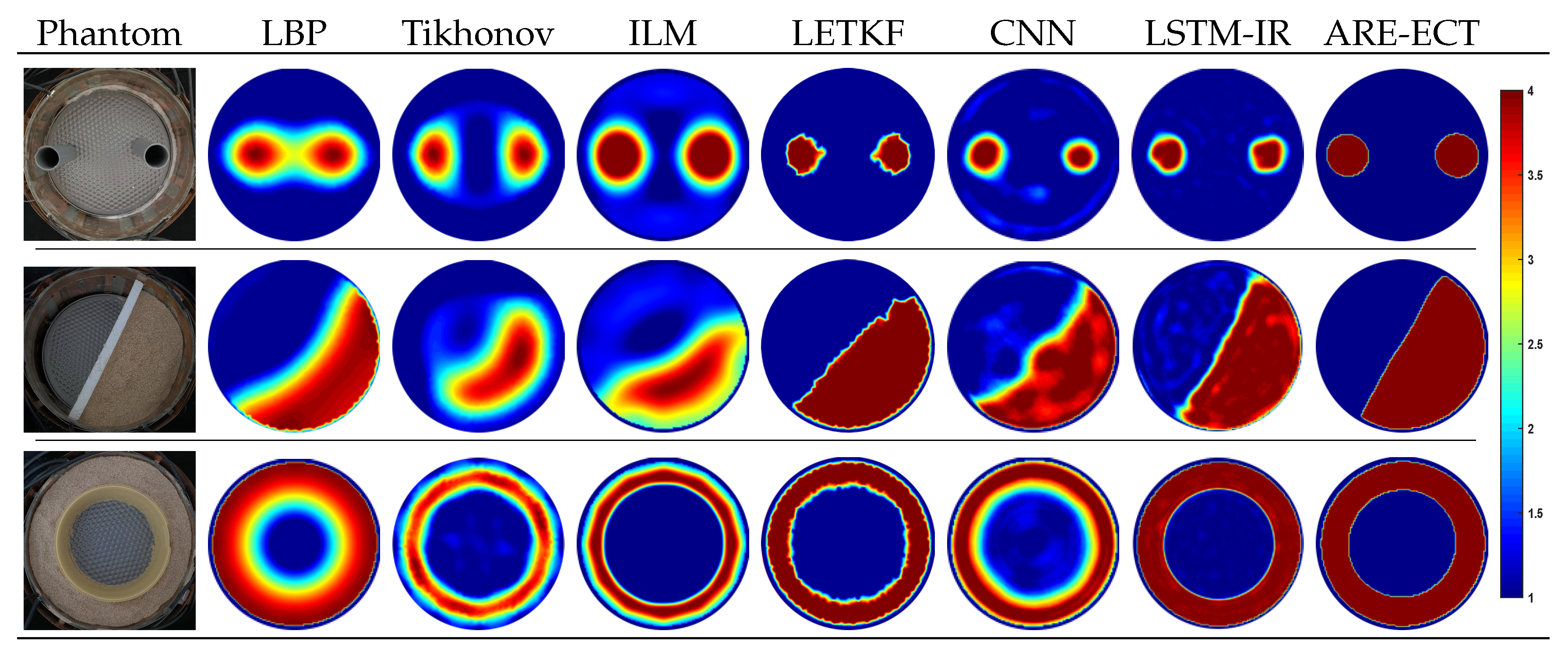
6.4. Evaluation Using Experimental Data
6.5. Computational Time Measure
7. Conclusions
Author Contributions
Funding
Acknowledgments
Conflicts of Interest
Abbreviations
| CT | Computed Tomography |
| ECT | Electrical Capacitance Tomography |
| ARE-ECT | Adversarial Resolution Enhancement |
| ILM | Iterative Landweber Method |
| LBP | Linear Back Projection |
| ML | Machine Learning |
| DNN | Deep Neural Networks |
| DL | Deep Learning |
| CNN | Convolutional Neural Network |
| LSTM | Long Short-Term Memory |
| CANN | Capacitance Artificial Neural Network |
| GCN | Graph Convolutional Networks |
| GAN | Generative Adversarial Network |
| CGAN | Conditional Generative Adversarial Network |
| LW | Landweber Algorithm |
| IE | Image Error |
| CC | Correlation Coefficient |
| LSTM-IR | Long Short-Term Memory Image Reconstruction |
| LETKF | Local Ensemble Transform Kalman Filter |
| ECVT | Electrical Capacitance Volume Tomography |
References
- Tsai, C.Y.; Feng, Y.C. Real-time multi-scale parallel compressive tracking. J.-Real-Time Image Process. 2019, 16, 2073–2091. [Google Scholar] [CrossRef]
- Xu, Z.; Yao, J.; Wang, Z.; Liu, Y.; Wang, H.; Chen, B.; Wu, H. Development of a Portable Electrical Impedance Tomography System for Biomedical Applications. IEEE Sens. J. 2018, 18, 8117–8124. [Google Scholar] [CrossRef]
- Xia, Z.; Cui, Z.; Chen, Y.; Hu, Y.; Wang, H. Generative adversarial networks for dual-modality electrical tomography in multi-phase flow measurement. Meas. J. Int. Meas. Confed. 2020, 173, 108608. [Google Scholar] [CrossRef]
- Wang, M. Industrial Tomography: Systems and Applications; Elsevier: Amsterdam, The Netherlands, 2015. [Google Scholar]
- Wang, H.; Yang, W. Scale-up of an electrical capacitance tomography sensor for imaging pharmaceutical fluidized beds and validation by computational fluid dynamics. Meas. Sci. Technol. 2011, 22, 104015. [Google Scholar] [CrossRef]
- Rymarczyk, T.; Kłosowski, G.; Kozłowski, E. A Non-Destructive System Based on Electrical Tomography and Machine Learning to Analyze the Moisture of Buildings. Sensors 2018, 18, 2285. [Google Scholar] [CrossRef] [Green Version]
- Cui, Z.; Wang, Q.; Xue, Q.; Fan, W.; Zhang, L.; Cao, Z.; Sun, B.; Wang, H. A review on image reconstruction algorithms for electrical capacitance/resistance tomography. Sens. Rev. 2016, 36, 429–445. [Google Scholar] [CrossRef]
- Sun, S.; Cao, Z.; Huang, A.; Xu, L.; Yang, W. A high-speed digital electrical capacitance tomography system combining digital recursive demodulation and parallel capacitance measurement. IEEE Sens. J. 2017, 17, 6690–6698. [Google Scholar] [CrossRef] [Green Version]
- Wang, Q.; Yang, C.; Wang, H.; Cui, Z.; Gao, Z. Online monitoring of gas–solid two-phase flow using projected CG method in ECT image reconstruction. Particuology 2013, 11, 204–215. [Google Scholar] [CrossRef]
- Raghavan, R.; Senior, P.; Wang, H.; Yang, W.; Duncan, S. Modelling, measurement and analysis of fluidised bed dryer using an ect sensor. In Proceedings of the 5th World Congress in Industrial Process Tomography. International Society for Industrial Process Tomography, Bergen, Norway, 3–6 September 2007; pp. 334–341. [Google Scholar]
- Yulei, Z.; Baolong, G.; Yunyi, Y. Latest development and analysis of electrical capacitance tomography technology. Chin. J. Sci. Instrum. 2012, 33, 1909–1920. [Google Scholar]
- Li, Y.; Yang, W. Image reconstruction by nonlinear Landweber iteration for complicated distributions. Meas. Sci. Technol. 2008, 19, 094014. [Google Scholar] [CrossRef]
- Chen, D.Y.; Chen, Y.; Wang, L.L.; Yu, X.Y. A Novel Gauss-Newton Image Reconstruction Algorithm for Electrical Capacitance Tomography System. Acta Electron. Sin. 2009, 4, 739–743. [Google Scholar]
- Vauhkonen, M.; Vadâsz, D.; Karjalainen, P.A.; Somersalo, E.; Kaipio, J.P. Tikhonov regularization and prior information in electrical impedance tomography. IEEE Trans. Med. Imaging 1998, 17, 285–293. [Google Scholar] [CrossRef] [PubMed]
- Gamio, J.; Ortiz-Aleman, C.; Martin, R. Electrical capacitance tomography two-phase oil-gas pipe flow imaging by the linear back-projection algorithm. Geofísica Int. 2005, 44, 265–273. [Google Scholar] [CrossRef]
- Zhang, W.; Wang, C.; Yang, W.; Wang, C.H. Application of electrical capacitance tomography in particulate process measurement–A review. Adv. Powder Technol. 2014, 25, 174–188. [Google Scholar] [CrossRef]
- Deabes, W.; Amin, H.H. Image Reconstruction Algorithm Based on PSO-Tuned Fuzzy Inference System for Electrical Capacitance Tomography. IEEE Access 2020, 8, 191875–191887. [Google Scholar] [CrossRef]
- Deabes, W.; Bouazza, K.E. Efficient Image Reconstruction Algorithm for ECT System Using Local Ensemble Transform Kalman Filter. IEEE Access 2021, 9, 12779–12790. [Google Scholar] [CrossRef]
- Xie, D.; Zhang, L.; Bai, L. Deep learning in visual computing and signal processing. Appl. Comput. Intell. Soft Comput. 2017, 2017, 1320780. [Google Scholar] [CrossRef]
- Zhu, H.; Sun, J.; Xu, L.; Tian, W.; Sun, S. Permittivity Reconstruction in Electrical Capacitance Tomography Based on Visual Representation of Deep Neural Network. IEEE Sens. J. 2020, 20, 4803–4815. [Google Scholar] [CrossRef]
- Yang, X.; Zhao, C.; Chen, B.; Zhang, M.; Li, Y. Big Data driven U-Net based Electrical Capacitance Image Reconstruction Algorithm. In Proceedings of the IST 2019—IEEE International Conference on Imaging Systems and Techniques, Abu Dhabi, United Arab Emirates, 9–10 December 2019. [Google Scholar] [CrossRef]
- Zheng, J.; Ma, H.; Peng, L. A CNN-based image reconstruction for electrical capacitance tomography. In Proceedings of the IEEE International Conference on Imaging Systems and Techniques, Abu Dhabi, United Arab Emirates, 9–10 December 2019; pp. 1–6. [Google Scholar] [CrossRef]
- Lili, W.; Xiao, L.; Deyun, C.; Hailu, Y.; Wang, C. ECT Image Reconstruction Algorithm Based on Multiscale Dual-Channel Convolutional Neural Network. Complexity 2020, 2020, 4918058. [Google Scholar] [CrossRef]
- Deabes, W.; Khayyat, K.M.J. Image Reconstruction in Electrical Capacitance Tomography Based on Deep Neural Networks. IEEE Sens. J. 2021, 21, 25818–25830. [Google Scholar] [CrossRef]
- Zheng, J.; Peng, L. An autoencoder-based image reconstruction for electrical capacitance tomography. IEEE Sens. J. 2018, 18, 5464–5474. [Google Scholar] [CrossRef]
- Deabes, W.; Sheta, A.; Bouazza, K.E.; Abdelrahman, M. Application of Electrical Capacitance Tomography for Imaging Conductive Materials in Industrial Processes. J. Sens. 2019, 2019, 4208349. [Google Scholar] [CrossRef]
- Deabes, W.; Sheta, A.; Braik, M. ECT-LSTM-RNN: An Electrical Capacitance Tomography Model-Based Long Short-Term Memory Recurrent Neural Networks for Conductive Materials. IEEE Access 2021, 9, 76325–76339. [Google Scholar] [CrossRef]
- Fabijańska, A.; Banasiak, R. Graph convolutional networks for enhanced resolution 3D Electrical Capacitance Tomography image reconstruction. Appl. Soft Comput. 2021, 110, 107608. [Google Scholar] [CrossRef]
- Goodfellow, I.; Pouget-Abadie, J.; Mirza, M.; Xu, B.; Warde-Farley, D.; Ozair, S.; Courville, A.; Bengio, Y. Generative Adversarial Nets. In Advances in Neural Information Processing Systems; Ghahramani, Z., Welling, M., Cortes, C., Lawrence, N., Weinberger, K.Q., Eds.; Curran Associates, Inc.: Red Hook, NY, USA, 2014; Volume 27. [Google Scholar]
- Mahdizadehaghdam, S.; Panahi, A.; Krim, H. Sparse generative adversarial network. In Proceedings of the IEEE/CVF International Conference on Computer Vision Workshops, Seoul, Korea, 27–28 October 2019. [Google Scholar]
- Xu, T.; Zhang, P.; Huang, Q.; Zhang, H.; Gan, Z.; Huang, X.; He, X. Attngan: Fine-grained text to image generation with attentional generative adversarial networks. In Proceedings of the IEEE Conference on Computer Vision and Pattern Recognition, Salt Lake City, UT, USA, 18–23 June 2018; pp. 1316–1324. [Google Scholar]
- Subramanian, S.; Mudumba, S.R.; Sordoni, A.; Trischler, A.; Courville, A.C.; Pal, C. Towards text generation with adversarially learned neural outlines. Adv. Neural Inf. Process. Syst. 2018, 31, 1–13. [Google Scholar]
- Mirsky, Y.; Lee, W. The creation and detection of deepfakes: A survey. Acm Comput. Surv. (CSUR) 2021, 54, 1–41. [Google Scholar] [CrossRef]
- Isola, P.; Zhu, J.Y.; Zhou, T.; Efros, A.A. Image-to-image translation with conditional adversarial networks. In Proceedings of the 30th IEEE Conference on Computer Vision and Pattern Recognition, CVPR, Honolulu, HI, USA, 21–26 July 2017; IEEE: Piscataway, NJ, USA, 2017; pp. 5967–5976. [Google Scholar] [CrossRef] [Green Version]
- Karras, T.; Laine, S.; Aittala, M.; Hellsten, J.; Lehtinen, J.; Aila, T. Analyzing and improving the image quality of stylegan. In Proceedings of the IEEE/CVF Conference on Computer Vision and Pattern Recognition, Seattle, WA, USA, 13–19 June 2020; pp. 8110–8119. [Google Scholar]
- Kim, S.W.; Zhou, Y.; Philion, J.; Torralba, A.; Fidler, S. Learning to simulate dynamic environments with gamegan. In Proceedings of the IEEE/CVF Conference on Computer Vision and Pattern Recognition, Seattle, WA, USA, 13–19 June 2020; pp. 1231–1240. [Google Scholar]
- Mirza, M.; Osindero, S. Conditional generative adversarial nets. arXiv 2014, arXiv:1411.1784. [Google Scholar]
- Selim, M.; Zhang, J.; Fei, B.; Zhang, G.Q.; Chen, J. STAN-CT: Standardizing CT Image using Generative Adversarial Networks. In AMIA Annual Symposium Proceedings; American Medical Informatics Association: Bethesda, MD, USA, 2020; Volume 2020, p. 1100. [Google Scholar]
- Yang, X.; Kahnt, M.; Brückner, D.; Schropp, A.; Fam, Y.; Becher, J.; Grunwaldt, J.D.; Sheppard, T.L.; Schroer, C.G. Tomographic reconstruction with a generative adversarial network. J. Synchrotron Radiat. 2020, 27, 486–493. [Google Scholar] [CrossRef]
- Liu, Z.; Bicer, T.; Kettimuthu, R.; Gursoy, D.; De Carlo, F.; Foster, I. TomoGAN: Low-dose synchrotron x-ray tomography with generative adversarial networks: Discussion. JOSA A 2020, 37, 422–434. [Google Scholar] [CrossRef] [Green Version]
- Ledig, C.; Theis, L.; Huszár, F.; Caballero, J.; Cunningham, A.; Acosta, A.; Aitken, A.; Tejani, A.; Totz, J.; Wang, Z.; et al. Photo-realistic single image super-resolution using a generative adversarial network. In Proceedings of the IEEE Conference on Computer Vision and Pattern Recognition, Honolulu, HI, USA, 21–26 July 2017; pp. 4681–4690. [Google Scholar]
- Lu, J.; Hu, W.; Sun, Y. A deep learning method for image super-resolution based on geometric similarity. Signal Process. Image Commun. 2019, 70, 210–219. [Google Scholar] [CrossRef]
- Ye, J.; Wang, H.; Yang, W. Image Reconstruction for Electrical Capacitance Tomography Based on Sparse Representation. IEEE Trans. Instrum. Meas. 2015, 64, 89–102. [Google Scholar] [CrossRef]
- Deabes, W.A.; Abdelrahman, M.A. A nonlinear fuzzy assisted image reconstruction algorithm for electrical capacitance tomography. Isa Trans. 2010, 49, 10–18. [Google Scholar] [CrossRef] [PubMed]
- Hitawala, S. Comparative study on generative adversarial networks. arXiv 2018, arXiv:1801.04271. [Google Scholar]
- Chakraborty, A.; Ragesh, R.; Shah, M.; Kwatra, N. S2cGAN: Semi-Supervised Training of Conditional GANs with Fewer Labels. arXiv 2020, arXiv:2010.12622. [Google Scholar]
- Qin, Z.; Shan, Y. Generation of Handwritten Numbers Using Generative Adversarial Networks. In Journal of Physics: Conference Series; IOP Publishing: Bristol, UK, 2021; Volume 1827, p. 012070. [Google Scholar]
- Ronneberger, O.; Fischer, P.; Brox, T. U-net: Convolutional networks for biomedical image segmentation. In International Conference on Medical Image Computing and Computer-Assisted Intervention; Springer: Berlin/Heidelberg, Germany, 2015; pp. 234–241. [Google Scholar]
- Abadi, M.; Agarwal, A.; Barham, P.; Brevdo, E.; Chen, Z.; Citro, C.; Corrado, G.S.; Davis, A.; Dean, J.; Devin, M.; et al. Tensorflow: Large-scale machine learning on heterogeneous distributed systems. arXiv 2016, arXiv:1603.04467. Available online: tensorflow.org (accessed on 8 April 2022).
- Chollet, F. Keras; GitHub: San Francisco, CA, USA, 2015; Available online: https://github.com/fchollet/keras (accessed on 12 February 2022).
- Tech4Imaging. Electrical Capacitance Volume Tomography. Ohio, USA. 2020. Available online: https://www.tech4imaging.com/ (accessed on 15 April 2022).


| GAN | CGAN | |
|---|---|---|
| Input | Latent vector | Random and auxiliary data |
| Output | Classify as real or generated | Classify labeled data as real or generated |
| Type | Unsupervised | Supervised |
| Data | No control over data | Conditional data |
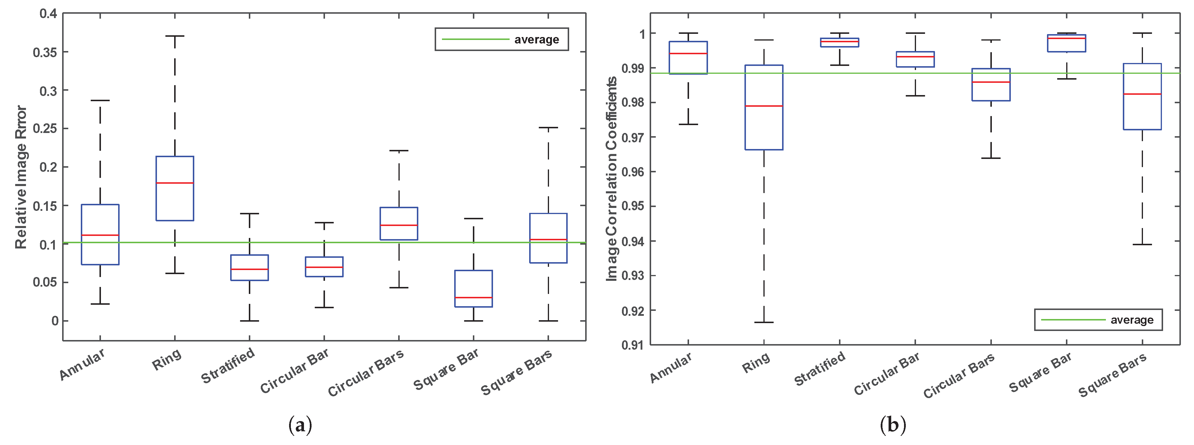
| Flow Patterns | Min. IE | Max. IE | Average IE | Min. CC | Max. CC | Average CC |
|---|---|---|---|---|---|---|
| Annular | 0.0219 | 0.2864 | 0.1160 | 0.9736 | 1.0000 | 0.9921 |
| Ring | 0.0562 | 0.3704 | 0.1781 | 0.9165 | 0.9980 | 0.9770 |
| Stratified | 0.0000 | 0.1395 | 0.0694 | 0.9907 | 1.0000 | 0.9970 |
| Single Cir. Bar | 0.0173 | 0.1276 | 0.0712 | 0.9819 | 1.0000 | 0.9923 |
| Multiple Cir. Bars | 0.0308 | 0.2178 | 0.1288 | 0.9639 | 0.9985 | 0.9845 |
| Single Sq. Bar | 0.0000 | 0.1329 | 0.0415 | 0.9868 | 1.0000 | 0.9965 |
| Multiple Sq. Bars | 0.0000 | 0.2512 | 0.1086 | 0.9390 | 1.0000 | 0.9803 |
| Total Average | IE | 0.1019 | CC | 0.9884 | ||
| Flow | LBP | Tikhonov | ILM | CNN | LSTM-IR | ARE-ECT | |
|---|---|---|---|---|---|---|---|
| Relative Image Error (IE) | Annular | 0.2412 | 0.1950 | 0.3351 | 0.1222 | 0.0561 | 0.0687 |
| Ring | 0.3776 | 0.1216 | 0.2984 | 0.2107 | 0.0989 | 0.0941 | |
| Stratified | 0.2590 | 0.6953 | 0.3203 | 0.3365 | 0.2032 | 0.1994 | |
| Cir. Bar | 0.3923 | 0.6562 | 0.6575 | 0.2224 | 0.1420 | 0.0821 | |
| 2 Cir. Bars | 0.4568 | 0.6638 | 0.4038 | 0.3274 | 0.1445 | 0.0990 | |
| 3 Cir. Bars | 0.6083 | 0.7492 | 0.4275 | 0.4765 | 0.2043 | 0.0940 | |
| Sq. Bar | 0.3677 | 0.5841 | 0.6575 | 0.2490 | 0.2122 | 0.0991 | |
| 2 Sq. Bars | 0.4988 | 0.3449 | 0.3294 | 0.3176 | 0.2415 | 0.1653 | |
| 3 Sq. Bars | 0.5112 | 0.6070 | 0.6909 | 0.4999 | 0.2558 | 0.0528 | |
| Correlation Coefficient (CC) | Annular | 0.8701 | 0.8885 | 0.9084 | 0.9590 | 0.9913 | 0.9864 |
| Ring | 0.8110 | 0.9792 | 0.9576 | 0.9396 | 0.9857 | 0.9870 | |
| Stratified | 0.9126 | 0.4232 | 0.9100 | 0.8200 | 0.9401 | 0.9587 | |
| Cir. Bar | 0.6964 | 0.7754 | 0.7974 | 0.8860 | 0.9541 | 0.9850 | |
| 2 Cir. Bars | 0.6681 | 0.8565 | 0.7963 | 0.8060 | 0.9640 | 0.9823 | |
| 3 Cir. Bars | 0.5498 | 0.5652 | 0.7625 | 0.7325 | 0.9363 | 0.9862 | |
| Sq. Bar | 0.8442 | 0.8264 | 0.6575 | 0.8997 | 0.9277 | 0.9850 | |
| 2 Sq. Bars | 0.7041 | 0.8326 | 0.8663 | 0.8527 | 0.9161 | 0.9617 | |
| 3 Sq. Bars | 0.5099 | 0.6361 | 0.5688 | 0.6668 | 0.8707 | 0.9951 |
| Phantom | IE | CC |
|---|---|---|
| 1 | 0.2601 | 0.9049 |
| 2 | 0.1847 | 0.9427 |
| 3 | 0.2761 | 0.8909 |
| 4 | 0.2816 | 0.8852 |
| LBP | Tikhonov | ILM | LETKF | CNN | LSTM-IR | ARE-ECT |
|---|---|---|---|---|---|---|
| 0.026 | 5.326 | 6.245 | 1.310 | 0.085 | 0.052 | 0.046 |
Publisher’s Note: MDPI stays neutral with regard to jurisdictional claims in published maps and institutional affiliations. |
© 2022 by the authors. Licensee MDPI, Basel, Switzerland. This article is an open access article distributed under the terms and conditions of the Creative Commons Attribution (CC BY) license (https://creativecommons.org/licenses/by/4.0/).
Share and Cite
Deabes, W.; Abdel-Hakim, A.E.; Bouazza, K.E.; Althobaiti, H. Adversarial Resolution Enhancement for Electrical Capacitance Tomography Image Reconstruction. Sensors 2022, 22, 3142. https://doi.org/10.3390/s22093142
Deabes W, Abdel-Hakim AE, Bouazza KE, Althobaiti H. Adversarial Resolution Enhancement for Electrical Capacitance Tomography Image Reconstruction. Sensors. 2022; 22(9):3142. https://doi.org/10.3390/s22093142
Chicago/Turabian StyleDeabes, Wael, Alaa E. Abdel-Hakim, Kheir Eddine Bouazza, and Hassan Althobaiti. 2022. "Adversarial Resolution Enhancement for Electrical Capacitance Tomography Image Reconstruction" Sensors 22, no. 9: 3142. https://doi.org/10.3390/s22093142
APA StyleDeabes, W., Abdel-Hakim, A. E., Bouazza, K. E., & Althobaiti, H. (2022). Adversarial Resolution Enhancement for Electrical Capacitance Tomography Image Reconstruction. Sensors, 22(9), 3142. https://doi.org/10.3390/s22093142