
Estimating Biomass and Carbon Sequestration Capacity of Phragmites australis Using Remote Sensing and Growth Dynamics Modeling: A Case Study in Beijing Hanshiqiao Wetland Nature Reserve, China


Abstract
1. Introduction
2. Methods
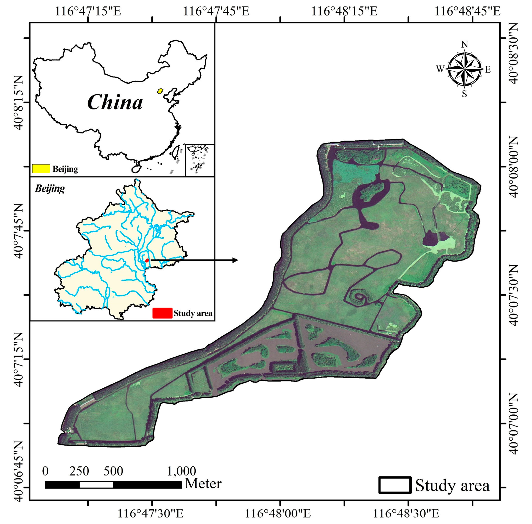
2.1. Study Site
2.2. Imagery Dataset
2.3. P. australis Growth Dynamics Model
2.3.1. Model Formulation
2.3.2. Model Calibration
2.3.3. Model Execution
2.4. P. australis Interpretation and AGB Retrieval
2.4.1. Preprocessing of Hyperspectral Images
2.4.2. Interpretation of P. australis
2.4.3. Retrieval of P. australis AGB
2.5. Evaluation of Carbon Sequestration Capacity
3. Results
3.1. Distribution and Retrieved AGB of P. australis
3.2. Calibration and Sensitivity Analysis of Growth Dynamics Model
- (1)
- The dates of the phenological points were calibrated based on the preliminary value obtained by the empirical relationships in Section 2.3.2. Most phenological points were moved backward to match the actual growth cycle of P. australis in the HWNR. The specific time of some representative phenological events during the growth cycle of P. australis is shown in Figure 4.
- (2)
- The constant of the nutrient availability and the biomass transfer rate from fertile leaf, sterile leaf, and peduncle to new rhizomes were slightly increased, and the respiration rate of above-ground organs was reduced in our model, to achieve higher peak biomass, as shown by the retrieved results.
- (3)
- The mortality rates of the above-ground organs at the onset of senescence, especially those of shoots and flowers, were increased after ts to match the occurrence of abrupt biomass loss at that stage.
3.3. Estimation of Carbon Sequestration Capacity
4. Discussion
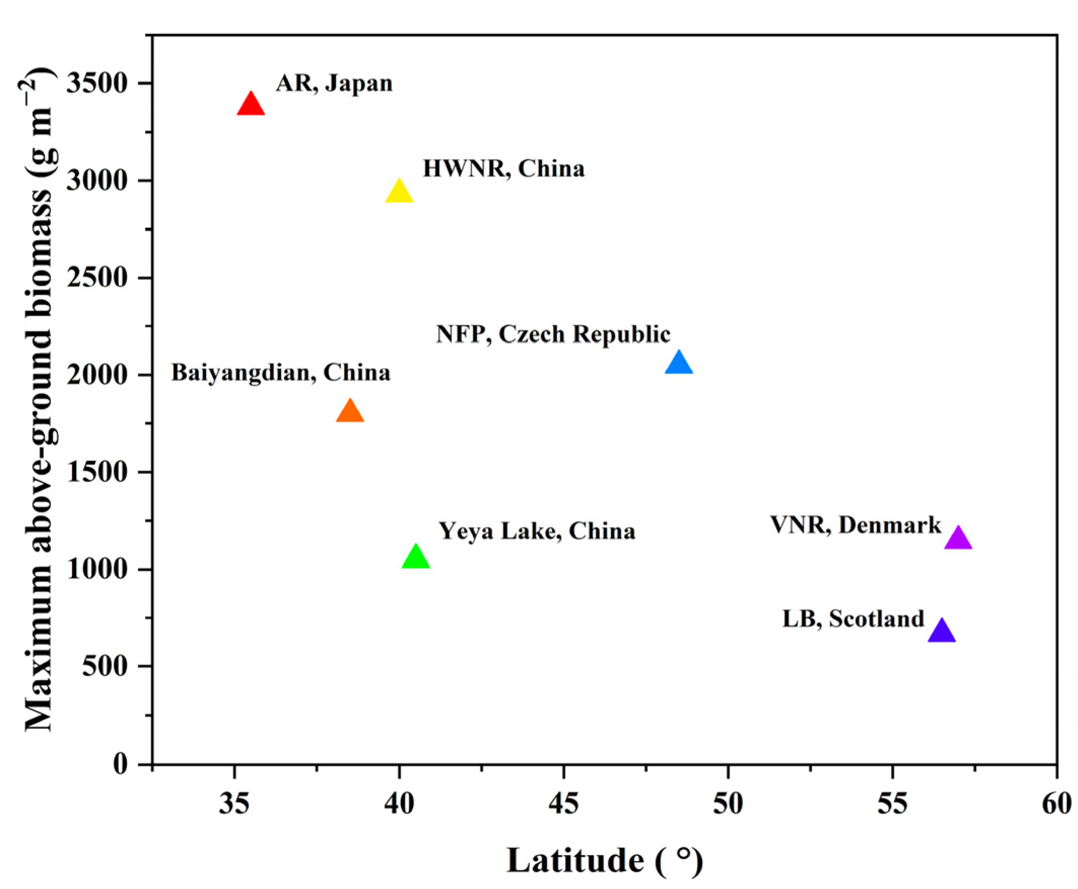
4.1. Comparison in Phenological Points and Biomass of P. australis from Other Sites
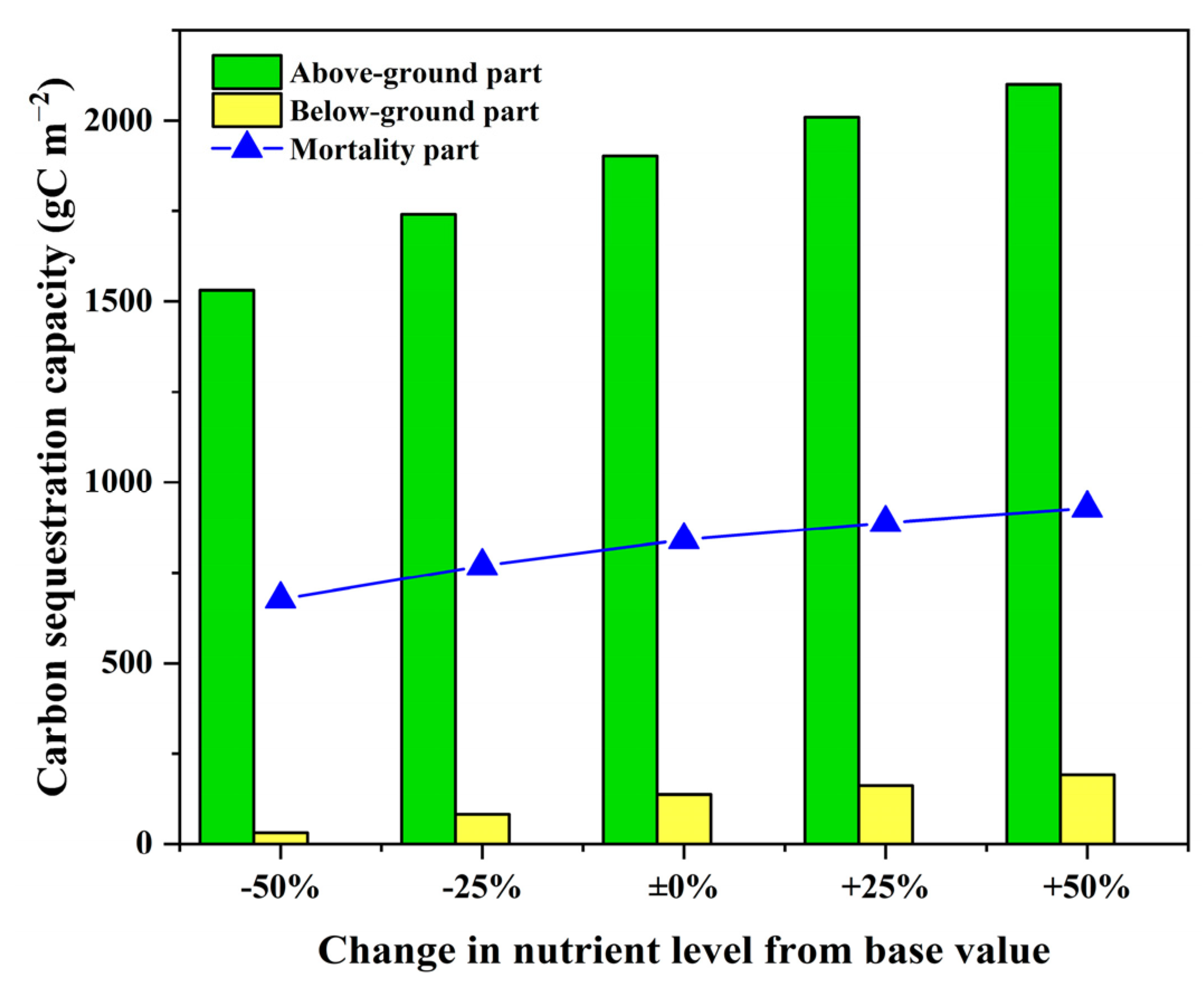
4.2. Influence of Nutrient Availability on Growth and Carbon Sequestration of P. australis
5. Conclusions
Supplementary Materials
Author Contributions
Funding
Institutional Review Board Statement
Informed Consent Statement
Data Availability Statement
Acknowledgments
Conflicts of Interest
References
- Holm, L.G.; Plucknett, D.L.; Pancho, J.V.; Herberger, J.P. The World’s Worst Weeds. In Distribution and Biology; University Press of Hawaii: Honolulu, HI, USA, 1977. [Google Scholar]
- White, D.A.; Visser, J.M. Water quality change in the Mississippi River, including a warming river, explains decades of wetland plant biomass change within its Balize delta. Aquat. Bot. 2016, 132, 5–11. [Google Scholar] [CrossRef]
- Schultz, R.E.; Pett, L. Plant community effects on CH4 fluxes, root surface area, and carbon storage in experimental wetlands. Ecol. Eng. 2018, 114, 96–103. [Google Scholar] [CrossRef]
- Duarte, C.M.; Losada, I.J.; Hendriks, I.E.; Mazarrasa, I.; Marba, N. The role of coastal plant communities for climate change mitigation and adaptation. Nat. Clim. Chang. 2013, 3, 961–968. [Google Scholar] [CrossRef]
- Zedler, J.B.; Kercher, S. Wetland resources: Status, trends, ecosystem services, and restorability. Annu. Rev. Environ. Resour. 2005, 30, 39–74. [Google Scholar] [CrossRef]
- Oteman, B.; Scrieciu, A.; Bouma, T.J.; Stanica, A.; Van Der Wal, D. Indicators of Expansion and Retreat of Phragmites Based on Optical and Radar Satellite Remote Sensing: A Case Study on the Danube Delta. Wetlands 2021, 41, 72. [Google Scholar] [CrossRef]
- Soetaert, K.; Hoffmann, M.; Meire, P.; Starink, M.; van Oevelen, D.; Van Regenmortel, S.; Cox, T. Modeling growth and carbon allocation in two reed beds (Phragmites australis) in the Scheldt estuary. Aquat. Bot. 2004, 79, 211–234. [Google Scholar] [CrossRef]
- Wan, R.; Wang, P.; Wang, X.; Yao, X.; Dai, X. Mapping aboveground biomass of four typical vegetation types in the Poyang Lake wetlands based on random forest modelling and landsat images. Front. Plant Sci. 2019, 10, 1281. [Google Scholar] [CrossRef]
- Dai, X.; Yang, G.; Liu, D.; Wan, R. Vegetation Carbon Sequestration Mapping in Herbaceous Wetlands by Using a MODIS EVI Time-Series Data Set: A Case in Poyang Lake Wetland, China. Remote Sens. 2020, 12, 3000. [Google Scholar] [CrossRef]
- Doughty, C.L.; Langley, J.A.; Walker, W.S.; Feller, I.C.; Schaub, R.; Chapman, S.K. Mangrove Range Expansion Rapidly Increases Coastal Wetland Carbon Storage. Estuaries Coast. 2016, 39, 385–396. [Google Scholar] [CrossRef]
- Simard, M.; Fatoyinbo, L.; Smetanka, C.; Rivera-Monroy, V.H.; Castaneda-Moya, E.; Thomas, N.; Van der Stocken, T. Mangrove canopy height globally related to precipitation, temperature and cyclone frequency. Nat. Geosci. 2019, 12, 40. [Google Scholar] [CrossRef]
- Arkebauer, T.J.; Chanton, J.P.; Verma, S.B.; Kim, J. Field measurements of internal pressurization in Phragmites australis (Poaceae) and implications for regulation of methane emissions in a midlatitude prairie wetland. Am. J. Bot. 2001, 88, 653–658. [Google Scholar] [CrossRef]
- Wolfer, S.R.; van Nes, E.H.; Straile, D. Modelling the clonal growth of the rhizomatous macrophyte Potamogeton perfoliatus. Ecol. Model. 2006, 192, 67–82. [Google Scholar] [CrossRef][Green Version]
- Asaeda, T.; Karunaratne, S. Dynamic modeling of the growth of Phragmites australis: Model description. Aquat. Bot. 2000, 68, 187. [Google Scholar] [CrossRef]
- Yi, Y.J.; Xie, H.Y.; Yang, Y.F.; Zhou, Y.; Yang, Z.F. Suitable habitat mathematical model of common reed (Phragmites australis) in shallow lakes with coupling cellular automaton and modified logistic function. Ecol. Model. 2020, 419, 108938. [Google Scholar] [CrossRef]
- Eid, E.M.; Shaltout, K.H.; Al-Sodany, Y.M.; Soetaert, K.; Jensen, K. Modeling Growth, Carbon Allocation and Nutrient Budgets of Phragmites australis in Lake Burullus, Egypt. Wetlands 2010, 30, 240–251. [Google Scholar] [CrossRef]
- Zheng, S.Y.; Shao, D.D.; Asaeda, T.; Sun, T.; Luo, S.X.; Cheng, M. Modeling the growth dynamics of Spartina alterniflora and the effects of its control measures. Ecol. Eng. 2016, 97, 144–156. [Google Scholar] [CrossRef]
- Asaeda, T.; Hai, D.N.; Manatunge, J.; Williams, D.; Roberts, J. Latitudinal characteristics of below- and above-ground biomass of Typha: A modelling approach. Ann. Bot. 2005, 96, 299–312. [Google Scholar] [CrossRef]
- Asaeda, T.; Sharma, P.; Rajapakse, L. Seasonal patterns of carbohydrate translocation and synthesis of structural carbon components in Typha angustifolia. Hydrobiologia 2008, 607, 87–101. [Google Scholar] [CrossRef]
- Wang, J.; Liu, Z.; Yu, H.; Li, F. Mapping Spartina alterniflora Biomass Using LiDAR and Hyperspectral Data. Remote Sens. 2017, 9, 589. [Google Scholar] [CrossRef]
- Moreau, S.; Le Toan, T. Biomass quantification of Andean wetland forages using ERS satellite SAR data for optimizing livestock management. Remote Sens. Environ. 2003, 84, 477–492. [Google Scholar] [CrossRef]
- Jensen, D.; Cavanaugh, K.C.; Simard, M.; Okin, G.S.; Castañeda-Moya, E.; McCall, A.; Twilley, R.R. Integrating imaging spectrometer and synthetic aperture radar data for estimating wetland vegetation aboveground biomass in coastal Louisiana. Remote Sens. 2019, 11, 2533. [Google Scholar] [CrossRef]
- Byrd, K.B.; O’Connell, J.L.; Di Tommaso, S.; Kelly, M. Evaluation of sensor types and environmental controls on mapping biomass of coastal marsh emergent vegetation. Remote Sens. Environ. 2014, 149, 166–180. [Google Scholar] [CrossRef]
- Mutanga, O.; Adam, E.; Cho, M.A. High density biomass estimation for wetland vegetation using WorldView-2 imagery and random forest regression algorithm. Int. J. Appl. Earth Obs. 2012, 18, 399–406. [Google Scholar] [CrossRef]
- Aslan, A.; Rahman, A.F.; Warren, M.W.; Robeson, S.M. Mapping spatial distribution and biomass of coastal wetland vegetation in Indonesian Papua by combining active and passive remotely sensed data. Remote Sens. Environ. 2016, 183, 65–81. [Google Scholar] [CrossRef]
- Luo, S.; Wang, C.; Xi, X.; Pan, F.; Qian, M.; Peng, D.; Nie, S.; Qin, H.; Lin, Y. Retrieving aboveground biomass of wetland Phragmites australis (common reed) using a combination of airborne discrete-return LiDAR and hyperspectral data. Int. J. Appl. Earth Obs. 2017, 58, 107–117. [Google Scholar] [CrossRef]
- Du, Y.; Wang, J.; Lin, Y.; Liu, Z.; Yu, H.; Yi, H. Estimating the Aboveground Biomass of Phragmites australis (Common Reed) Based on Multi-Source Data. In Proceedings of the 38th IEEE International Geoscience and Remote Sensing Symposium (IGARSS), Valencia, Spain, 22–27 July 2018; pp. 9241–9244. [Google Scholar]
- Zhao, Y.W.; Liu, Y.X.; Wu, S.R.; Li, Z.M.; Zhang, Y.; Qin, Y.; Yin, X.A. Construction and application of an aquatic ecological model for an emergent-macrophyte-dominated wetland: A case of Hanshiqiao wetland. Ecol. Eng. 2016, 96, 214–223. [Google Scholar] [CrossRef]
- Lei, T.; Cui, G.; Chen, J.; Zhang, J.; Chen, Y.; Wang, D.; Chen, Y. Diversity and priority conservation graded wetland vascular plants in Beijing. Acta Ecol. Sin. 2006, 26, 1675–1685. [Google Scholar]
- Wei, J.; Cui, L.; Li, W.; Lei, Y.; Ping, Y.; Sun, B.; Yu, J.; Liang, Z. Nitrogen and phosphorus removal effect in subsurface constructed wetland under low temperature condition. Ecol. Sci. 2017, 36, 43–47. [Google Scholar]
- Li, C.; Huang, Y.; Guo, H.; Wu, G.; Wang, Y.; Li, W.; Cui, L. The Concentrations and Removal Effects of PM10 and PM2.5 on a Wetland in Beijing. Sustainability 2019, 11, 1312. [Google Scholar] [CrossRef]
- Hu, J.; Wu, J.; Zhao, C.; Wang, P. Challenges for China to achieve carbon neutrality and carbon peak goals: Beijing case study. PLoS ONE 2021, 16, e0258691. [Google Scholar] [CrossRef]
- Li, W.; Dou, Z.; Wang, Y.; Wu, G.; Zhang, M.; Lei, Y.; Ping, Y.; Wang, J.; Cui, L.; Ma, W. Estimation of above-ground biomass of reed (Phragmites communis) based on in situ hyperspectral data in Beijing Hanshiqiao Wetland, China. Wetl. Ecol. Manag. 2018, 27, 87–102. [Google Scholar] [CrossRef]
- Lu, S.; Shimizu, Y.; Ishii, J.; Funakoshi, S.; Washitani, I.; Omasa, K. Estimation of abundance and distribution of two moist tall grasses in the Watarase wetland, Japan, using hyperspectral imagery. ISPRS J. Photogramm. 2009, 64, 674–682. [Google Scholar] [CrossRef]
- Li, Q.; Zhong, R.; Wang, Y. A Method for the Destriping of an Orbita Hyperspectral Image with Adaptive Moment Matching and Unidirectional Total Variation. Remote Sens. 2019, 11, 2098. [Google Scholar] [CrossRef]
- Jiang, Y.; Wang, J.; Zhang, L.; Zhang, G.; Li, X.; Wu, J. Geometric Processing and Accuracy Verification of Zhuhai-1 Hyperspectral Satellites. Remote Sens. 2019, 11, 996. [Google Scholar] [CrossRef]
- Besnard, A.G.; Davranche, A.; Maugenest, S.; Bouzille, J.B.; Vian, A.; Secondi, J. Vegetation maps based on remote sensing are informative predictors of habitat selection of grassland birds across a wetness gradient. Ecol. Indic. 2015, 58, 47–54. [Google Scholar] [CrossRef]
- Everitt, J.H.; Yang, C.; Fletcher, R.; Deloach, C.J. Comparison of QuickBird and SPOT 5 satellite imagery for mapping giant reed. J. Aquat. Plant. Manag. 2008, 46, 77–82. [Google Scholar]
- Cui, Y.; Li, S.; Wu, W.; Liu, M. The application of dam break monitoring based on BJ-2 images. In Proceedings of the 10th International Symposium on Multispectral Image Processing and Pattern Recognition (MIPPR)—Remote Sensing Image Processing, Geographic Information Systems, and Other Applications, Xiangyang, China, 28–29 October 2017. [Google Scholar]
- Fu, X.; Zhu, Q.; Liu, C.; Li, N.; Zhuang, W.; Yang, Z.; Lu, H.; Tang, M. Estimation of Landslides and Road Capacity after August 8, 2017, MS7.0 Jiuzhaigou Earthquake Using High-Resolution Remote Sensing Images. Adv. Civ. Eng. 2020, 2020, 8828385. [Google Scholar] [CrossRef]
- Dong, L.; Li, X.; Wang, G.; Sun, Q. Change Detection Method of Construction Land Based on Multiple Feature Fusion. Remote Sens. Infor. 2017, 32, 152–156. [Google Scholar]
- Forsythe, W.C.; Rykiel, E.J.; Stahl, R.S.; Wu, H.-i.; Schoolfield, R.M. A Model Comparison for Daylength as a Function of Latitude and Day of Year. Ecol. Model. 1995, 80, 87–95. [Google Scholar] [CrossRef]
- Cui, L.; Zuo, X.; Dou, Z.; Huang, Y.; Zhao, X.; Zhai, X.; Lei, Y.; Li, J.; Pan, X.; Li, W. Plant identification of Beijing Hanshiqiao wetland based on hyperspectral data. Spectrosc. Lett. 2021, 54, 381–394. [Google Scholar] [CrossRef]
- Zhang, W.W.; Yao, L.; Li, H.; Sun, D.F.; Zhou, L.D. Research on Land Use Change in Beijing Hanshiqiao Wetland Nature Reserve Using Remote Sensing and GIS. In Proceedings of the 3rd International Conference on Environmental Science and Information Application Technology (ESIAT), Xian, China, 20–21 August 2011; pp. 583–588. [Google Scholar]
- Meng, S.; Wang, X.; Hu, X.; Luo, C.; Zhong, Y. Deep learning-based crop mapping in the cloudy season using one-shot hyperspectral satellite imagery. Comput. Electron. Agric. 2021, 186, 106188. [Google Scholar] [CrossRef]
- Cooley, T.; Anderson, G.P.; Felde, G.W.; Hoke, M.L.; Ratkowski, A.J.; Chetwynd, J.H.; Gardner, J.A.; Adler-Golden, S.M.; Matthew, M.W.; Berk, A.; et al. FLAASH, a MODTRAN4-based atmospheric correction algorithm, its application and validation. In Proceedings of the IEEE International Geoscience and Remote Sensing Symposium (IGARSS 2002)/24th Canadian Symposium on Remote Sensing, Toronto, ON, Canada, 24–28 June 2002; pp. 1414–1418. [Google Scholar]
- Goyal, M.K.; Panchariya, V.K.; Sharma, A.; Singh, V. Comparative Assessment of SWAT Model Performance in two Distinct Catchments under Various DEM Scenarios of Varying Resolution, Sources and Resampling Methods. Water Resour. Manag. 2018, 32, 805–825. [Google Scholar] [CrossRef]
- Zhang, J.; Chen, Y.; Lei, T.; Chen, J.; Cui, G. Inter-specific Relations of the Dominant Plant Populations in the Hanshiqiao Wetland in Beijing. Wetl. Sci. 2007, 5, 146–152. [Google Scholar]
- Liu, S.; Hong, J.; Hu, D.; Jiang, Z. Vegetation Classification and the Change of Vegetation Pattern from 2003 to 2006 in the Hanshiqiao Wetland Nature Reserve, Beijing. Wetl. Sci. 2008, 6, 19–28. [Google Scholar]
- Mahmud, M.R.; Numata, S.; Hosaka, T. Mapping an invasive goldenrod of Solidago altissima in urban landscape of Japan using multi-scale remote sensing and knowledge-based classification. Ecol. Indic. 2020, 111, 105975. [Google Scholar] [CrossRef]
- Yang, C.; Goolsby, J.A.; Everitt, J.H.; Du, Q. Applying six classifiers to airborne hyperspectral imagery for detecting giant reed. Geocarto Int. 2012, 27, 413–424. [Google Scholar] [CrossRef]
- Munoz-Mari, J.; Bovolo, F.; Gomez-Chova, L.; Bruzzone, L.; Camps-Valls, G. Semisupervised One-Class Support Vector Machines for Classification of Remote Sensing Data. IEEE Trans. Geosci. Remote 2010, 48, 3188–3197. [Google Scholar] [CrossRef]
- Smola, A.J.; Scholkopf, B. A tutorial on support vector regression. Stat. Comput. 2004, 14, 199–222. [Google Scholar] [CrossRef]
- Cao, J.; Leng, W.; Liu, K.; Liu, L.; He, Z.; Zhu, Y. Object-Based Mangrove Species Classification Using Unmanned Aerial Vehicle Hyperspectral Images and Digital Surface Models. Remote Sens. 2018, 10, 89. [Google Scholar] [CrossRef]
- Lin, C.; Wu, C.-C.; Tsogt, K.; Ouyang, Y.-C.; Chang, C.-I. Effects of atmospheric correction and pansharpening on LULC classification accuracy using WorldView-2 imagery. Inf. Process. Agric. 2015, 2, 25–36. [Google Scholar] [CrossRef]
- Lambert, M.-J.; Traoré, P.C.S.; Blaes, X.; Baret, P.; Defourny, P. Estimating smallholder crops production at village level from Sentinel-2 time series in Mali’s cotton belt. Remote Sens. Environ. 2018, 216, 647–657. [Google Scholar] [CrossRef]
- Dong, G.; Bai, J.; Yang, S.; Wu, L.; Cai, M.; Zhang, Y.; Luo, Y.; Wang, Z. The impact of land use and land cover change on net primary productivity on China’s Sanjiang Plain. Environ. Earth Sci. 2015, 74, 2907–2917. [Google Scholar] [CrossRef]
- Noormets, A.; Bracho, R.; Ward, E.; Seiler, J.; Strahm, B.; Lin, W.; McElligott, K.; Domec, J.C.; Gonzalez-Benecke, C.; Jokela, E.J.; et al. Heterotrophic Respiration and the Divergence of Productivity and Carbon Sequestration. Geophys. Res. Lett. 2021, 48, e2020GL092366. [Google Scholar] [CrossRef]
- Karunaratne, S.; Asaeda, T.; Yutani, K. Growth performance of Phragmites australis in Japan: Influence of geographic gradient. Environ. Exp. Bot. 2003, 50, 51–66. [Google Scholar] [CrossRef]
- Clevering, O.A.; Brix, H.; Lukavska, J. Geographic variation in growth responses in Phragmites australis. Aquat. Bot. 2001, 69, 89–108. [Google Scholar] [CrossRef]
- Zhao, Y.; Yang, Z.; Xia, X.; Wang, F. A shallow lake remediation regime with Phragmites australis: Incorporating nutrient removal and water evapotranspiration. Water Res. 2012, 46, 5635–5644. [Google Scholar] [CrossRef]
- Wu, H.F.; Wang, Z. Analysis on Spatial and Temporal Dynamic of Biomass of Phragmitesaustralis in Yeya Lake Wetland. J. Cap. Norm. Univ. 2014, 35, 51–55. [Google Scholar] [CrossRef]
- Vymazal, J.; Krőpfelová, L. Growth of Phragmites australis and Phalaris arundinacea in constructed wetlands for wastewater treatment in the Czech Republic. Ecol. Eng. 2005, 25, 606–621. [Google Scholar] [CrossRef]
- Dykyjová, D.; Hradecká, D. Production ecology of Phragmites communis 1. Relations of two ecotypes to the microclimate and nutrient conditions of habitat. Folia Geobot. Phytotaxon. 1976, 11, 23–61. [Google Scholar] [CrossRef]
- Zhao, Y.; Xia, X.H.; Yang, Z.F. Growth and nutrient accumulation of Phragmites australis in relation to water level variation and nutrient loadings in a shallow lake. J. Environ. Sci. 2013, 25, 16–25. [Google Scholar] [CrossRef]
- Hua, Y.Y.; Cui, B.S.; He, W.J.; Liu, Y.L. Optimum water depth threshold in reed marsh areas of the Yellow River Delta, China. In Proceedings of the 18th Biennial ISEM Conference on Ecological Modelling for Global Change and Coupled Human and Natural Systems, Beijing, China, 20–23 September 2011; pp. 1820–1826. [Google Scholar]
- Ho, Y.B. Shoot Development and Production Studies of Phragmites australis (Cav) Trin Ex Steudel in Scottish Lochs. Hydrobiologia 1979, 64, 215–222. [Google Scholar] [CrossRef]
- Schierup, H.-H.; Larsen, V.J. Macrophyte cycling of zinc, copper, lead and cadmium in the littoral zone of a polluted and a non-polluted lake. I. Availability, uptake and translocation of heavy metals in Phragmites australis (Cav.) Trin. Aquat. Bot. 1981, 11, 197–210. [Google Scholar] [CrossRef]
- Ksenofontova, T. General Changes in the Matsalu Bay Reedbeds in This Century and Their Present Quality (Estonian Ssr). Aquat. Bot. 1989, 35, 111–120. [Google Scholar] [CrossRef]
- Wang, X.; Zhang, D.; Guan, B.; Qi, Q.; Tong, S. Optimum water supplement strategy to restore reed wetland in the Yellow River Delta. PLoS ONE 2017, 12, e0177692. [Google Scholar] [CrossRef]
- Hardej, M.; Ozimek, T. The effect of sewage sludge flooding on growth and morphometric parameters of Phragmites australis (Cav.) Trin. ex Steudel. Ecol. Eng. 2002, 18, 343–350. [Google Scholar] [CrossRef]
- Eid, E.M.; Shaltout, K.H.; Al-Sodany, Y.M.; Haroun, S.A.; Jensen, K. A comparison of the functional traits of Phragmites australis in Lake Burullus (a Ramsar site in Egypt): Young vs. old populations over the nutrient availability gradient. Ecol. Eng. 2021, 166, 106244. [Google Scholar] [CrossRef]
- Tan, Y.; Li, J.; Cheng, J.; Gu, B.; Hong, J. The sinks of dissolved inorganic nitrogen in surface water of wetland mesocosms. Ecol. Eng. 2013, 52, 125–129. [Google Scholar] [CrossRef]
- Wu, S.; Xu, M.; Chen, Y.; Liu, Y.; Li, Z.; Zhao, Y. Evaluation of eutrophication for the Hanshiqiao wetland based on water quality and plankton data. Acta Sci. Circumst. 2015, 35, 411–417. [Google Scholar]
- Pacheco, F.; Roland, F.; Downing, J. Eutrophication reverses whole-lake carbon budgets. Inland Waters 2014, 4, 41–48. [Google Scholar] [CrossRef]
- Grasset, C.; Abril, G.; Guillard, L.; Delolme, C.; Bornette, G. Carbon emission along a eutrophication gradient in temperate riverine wetlands: Effect of primary productivity and plant community composition. Freshw. Biol. 2016, 61, 1405–1420. [Google Scholar] [CrossRef]
- Gonzalez-Alcaraz, M.N.; Egea, C.; Jimenez-Carceles, F.J.; Parraga, I.; Maria-Cervantes, A.; Delgado, M.J.; Alvarez-Rogel, J. Storage of organic carbon, nitrogen and phosphorus in the soil-plant system of Phragmites australis stands from a eutrophicated Mediterranean salt marsh. Geoderma 2012, 185, 61–72. [Google Scholar] [CrossRef]
- Carmichael, M.J.; Bernhardt, E.S.; Braeuer, S.L.; Smith, W.K. The role of vegetation in methane flux to the atmosphere: Should vegetation be included as a distinct category in the global methane budget? Biogeochemistry 2014, 119, 1–24. [Google Scholar] [CrossRef]
- Kiedrzynska, E.; Wagner, I.; Zalewski, M. Quantification of phosphorus retention efficiency by floodplain vegetation and a management strategy for a eutrophic reservoir restoration. Ecol. Eng. 2008, 33, 15–25. [Google Scholar] [CrossRef]
- Were, D.; Kansiime, F.; Fetahi, T.; Cooper, A.; Jjuuko, C. Carbon Sequestration by Wetlands: A Critical Review of Enhancement Measures for Climate Change Mitigation. Earth Syst. Environ. 2019, 3, 327–340. [Google Scholar] [CrossRef]


| Parameter | Value |
|---|---|
| Spatial resolution | 10 m |
| Swath width | 150 × 150 km |
| Satellite mass | 67 kg |
| Sensor height | 500 km |
| On-orbit life span | >5 years |
| Signal-to-noise ratio | >30 |
| Wavelength | 400 nm to 1000 nm |
| Spectral resolution | 2.5 nm |
| Bands | 256 (32 bands can be selected) |
| Revisit cycle | 5 days |
| Phenological Points | Phenological Events |
|---|---|
| tr | The formation of new roots and fertile leaves, as well as the beginning of translocation of dry matter from old rhizomes to fertile leaves and roots |
| tb | The formation of sterile leaves and non-flowering secondary shoots, as well as the beginning of translocation of dry matter from old rhizomes to sterile leaves and non-flowering secondary shoots |
| tp | The formation of new rhizomes and peduncles, together with the beginning of translocation of dry matter from old rhizomes to peduncles, as well as the beginning of translocation of photosynthesized material to below-ground plant organs |
| tf | The appearance of panicles as well as the beginning of translocation of dry matter and photosynthesized material from peduncles to panicles |
| te | The ending of mobilization of dry matter from rhizomes to shoots and roots |
| ts | The commencement of shoot senescence, together with the beginning of translocation of accumulated shoot dry matter to below-ground organs |
| Parameter | Training Samples | Validation Samples | Total |
|---|---|---|---|
| Water body | 74 | 32 | 106 |
| P. australis | 59 | 33 | 92 |
| N. tetragona | 14 | 10 | 24 |
| T. orientalis | 15 | 11 | 26 |
| Other vegetation | 75 | 21 | 96 |
| Class | JM Value | TD Value |
|---|---|---|
| Water body | 1.97 | 1.99 |
| N. tetragona | 1.99 | 2 |
| T. orientalis | 1.99 | 2 |
| Other vegetation | 1.98 | 1.99 |
| Class | Producer’s Accuracy (PA) | User’s Accuracy (UA) |
|---|---|---|
| Water body | 87.67% | 82.40% |
| P. australis | 94.71% | 96.95% |
| T. orientalis | 70.89% | 81.05% |
| N. tetragona | 75.87% | 71.10% |
| Other vegetation | 94.45% | 94.78% |
| Overall accuracy | 92.21% | |
| Kappa coefficient | 0.88 | |
| Parameters | Variation (%) | AGB (%) |
| Maximum specific net daily photosynthesis rate | +50 | +56.35% |
| −50 | −58.01% | |
| Specific mortality rate of shoots | +50 | −17.14% |
| −50 | +21.46% | |
| Fraction of shoot transfer to rhizome | +50 | −12.41% |
| −50 | +14.73% | |
| Constant of the availability of nutrients | +50 | +8.95% |
| −50 | −17.38% | |
| Fraction of shoot biomass for elongation | +50 | +7.08% |
| −50 | −13.48% |
| Parameter | Region | ||||
|---|---|---|---|---|---|
| AR | HWNR | NFP | LB | VNR | |
| Latitude | 35°51′ N | 40°06′ N | 48°48′ N | 56°65′ N | 57°05′ N |
| Primary shoot growth start (J-day) | 93 | 140 | 110 | 83 | 100 |
| Panicle appearance (J-day) | 213 | 225 | 196 | 213 | 232 |
| Maximum above-ground biomass (g/m2) | 3379.6 | 2930.1 | 2050 | 669 | 1145.6 |
Publisher’s Note: MDPI stays neutral with regard to jurisdictional claims in published maps and institutional affiliations. |
© 2022 by the authors. Licensee MDPI, Basel, Switzerland. This article is an open access article distributed under the terms and conditions of the Creative Commons Attribution (CC BY) license (https://creativecommons.org/licenses/by/4.0/).
Share and Cite
Wang, S.; Li, S.; Zheng, S.; Gao, W.; Zhang, Y.; Cao, B.; Cui, B.; Shao, D. Estimating Biomass and Carbon Sequestration Capacity of Phragmites australis Using Remote Sensing and Growth Dynamics Modeling: A Case Study in Beijing Hanshiqiao Wetland Nature Reserve, China. Sensors 2022, 22, 3141. https://doi.org/10.3390/s22093141
Wang S, Li S, Zheng S, Gao W, Zhang Y, Cao B, Cui B, Shao D. Estimating Biomass and Carbon Sequestration Capacity of Phragmites australis Using Remote Sensing and Growth Dynamics Modeling: A Case Study in Beijing Hanshiqiao Wetland Nature Reserve, China. Sensors. 2022; 22(9):3141. https://doi.org/10.3390/s22093141
Chicago/Turabian StyleWang, Siyuan, Sida Li, Shaoyan Zheng, Weilun Gao, Yong Zhang, Bo Cao, Baoshan Cui, and Dongdong Shao. 2022. "Estimating Biomass and Carbon Sequestration Capacity of Phragmites australis Using Remote Sensing and Growth Dynamics Modeling: A Case Study in Beijing Hanshiqiao Wetland Nature Reserve, China" Sensors 22, no. 9: 3141. https://doi.org/10.3390/s22093141
APA StyleWang, S., Li, S., Zheng, S., Gao, W., Zhang, Y., Cao, B., Cui, B., & Shao, D. (2022). Estimating Biomass and Carbon Sequestration Capacity of Phragmites australis Using Remote Sensing and Growth Dynamics Modeling: A Case Study in Beijing Hanshiqiao Wetland Nature Reserve, China. Sensors, 22(9), 3141. https://doi.org/10.3390/s22093141