
Can Hyperspectral Imaging and Neural Network Classification Be Used for Ore Grade Discrimination at the Point of Excavation?

 ,
,  , and
, and
Abstract
:1. Introduction
2. Materials and Methods
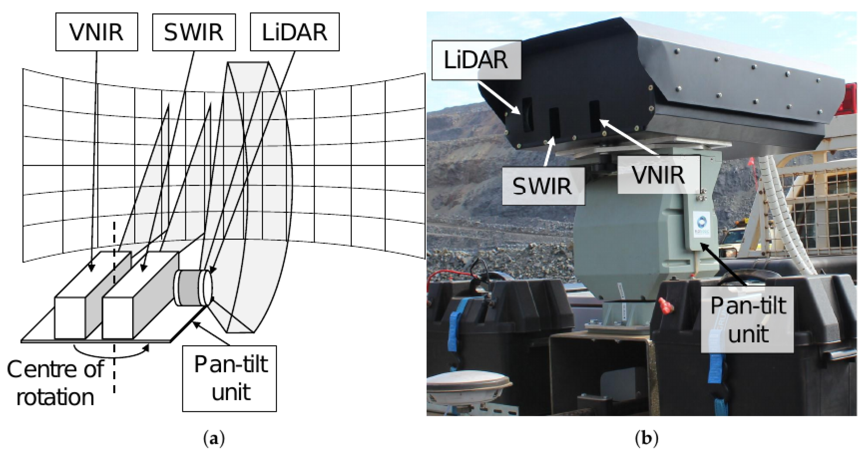
2.1. Hardware
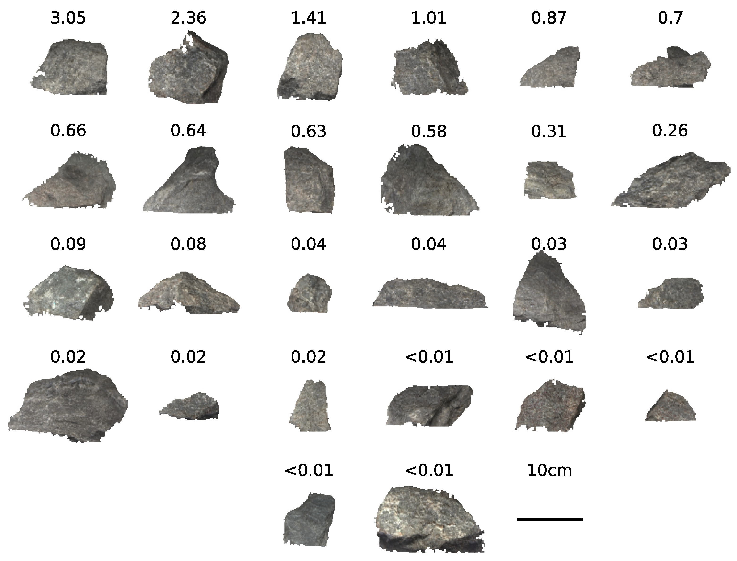
2.2. Fieldwork
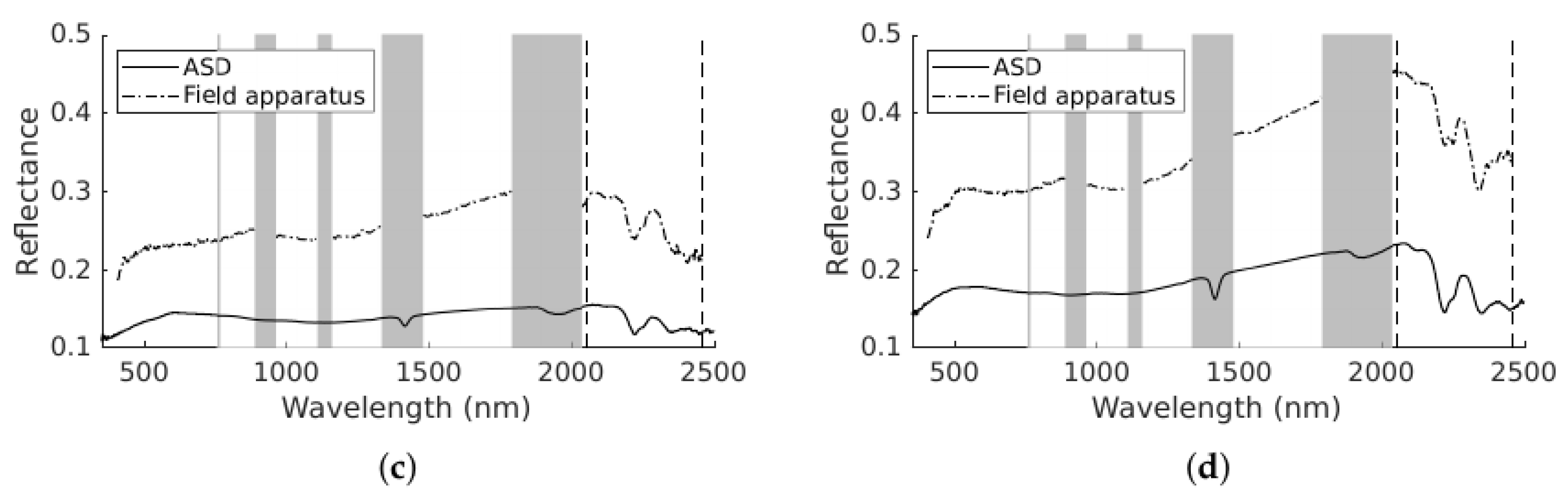
2.3. Data Preprocessing
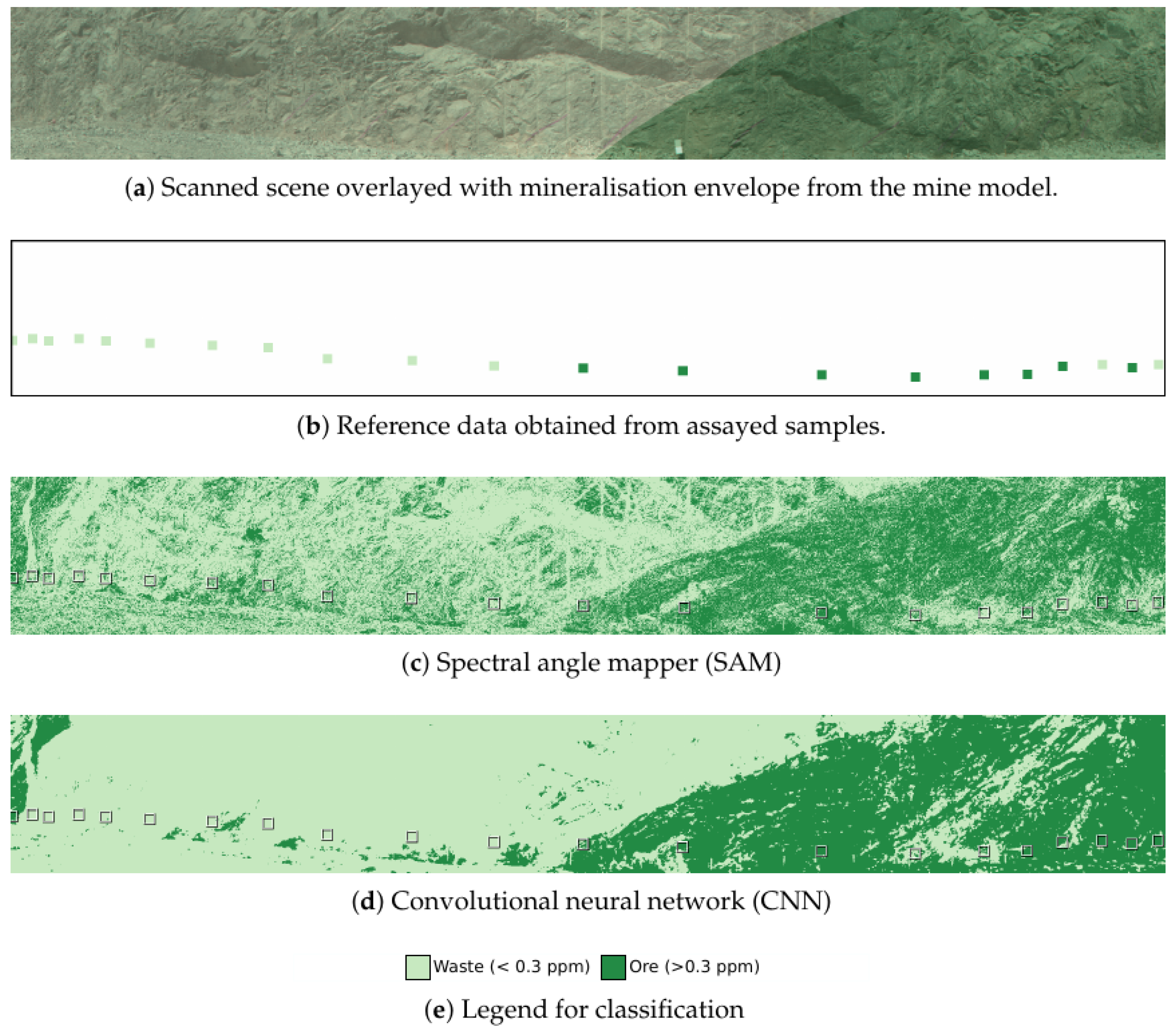
2.4. Classification
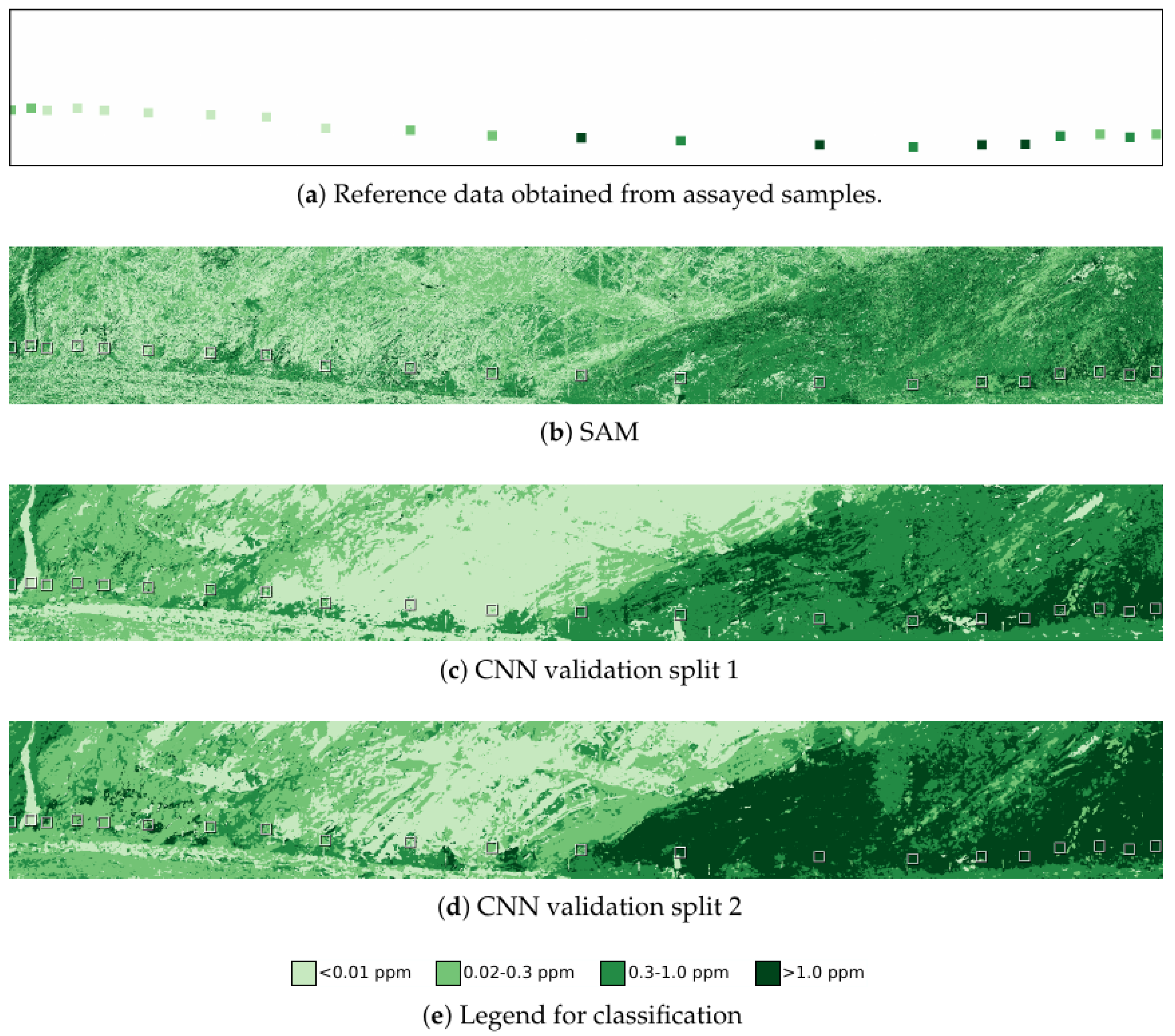
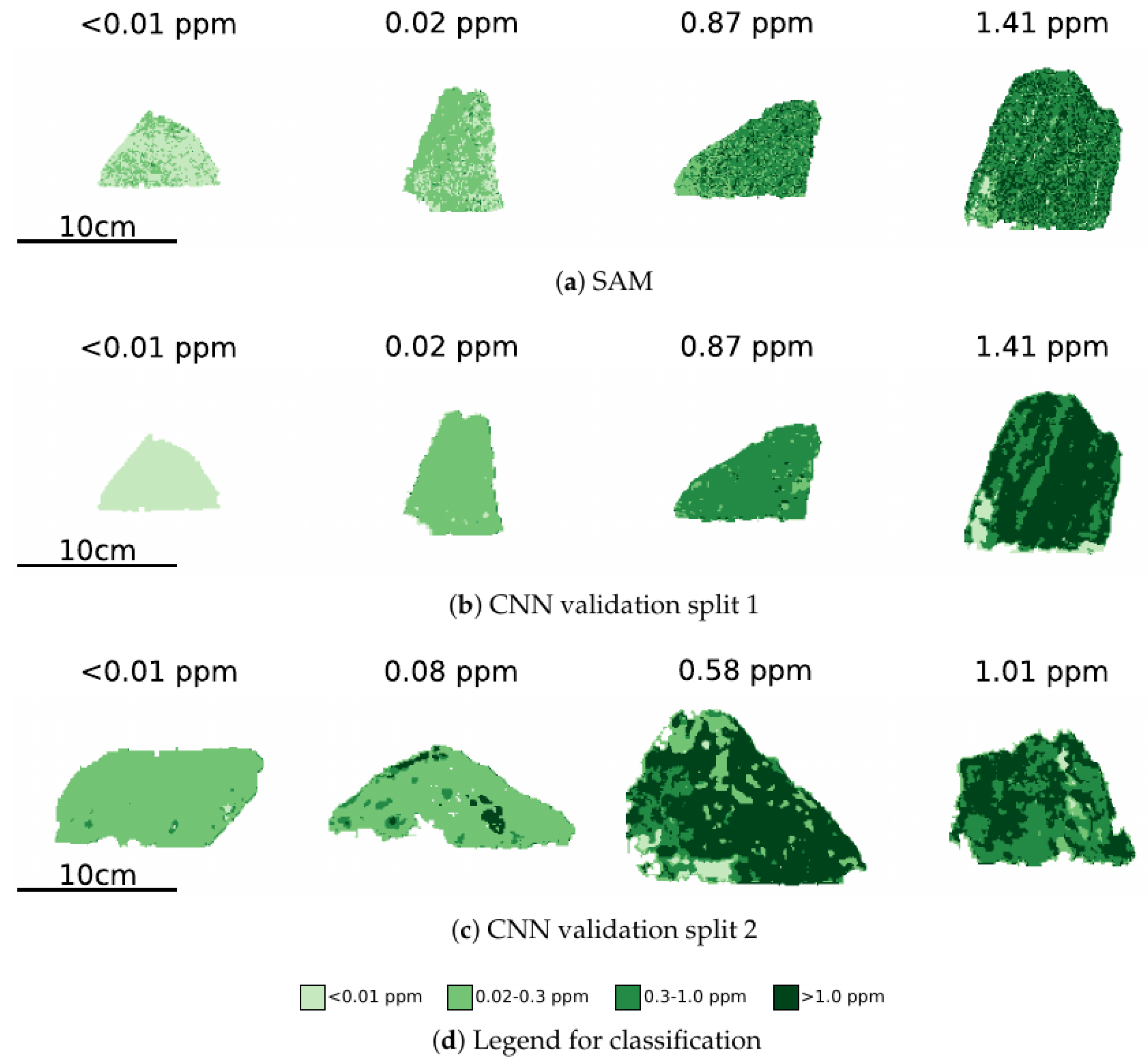
3. Results
4. Discussion
5. Conclusions
Author Contributions
Funding
Institutional Review Board Statement
Informed Consent Statement
Data Availability Statement
Conflicts of Interest
Abbreviations
| CNN | Convolutional neural network |
| DOF | Degree of freedom |
| FOV | Field of view |
| LiDAR | Light detection and ranging |
| OA | Overall accuracy |
| RTK GNSS | Real-time kinematic global navigation satellite system |
| SAM | Spectral angle mapper |
| SWIR | Short-wavelength infrared |
| VNIR | Visible-near-infrared |
References
- Goetz, A.F. Three decades of hyperspectral remote sensing of the Earth: A personal view. Remote Sens. Environ. 2009, 113 (Suppl. 1), S5–S16. [Google Scholar] [CrossRef]
- Hunt, G.R. Spectral Signature of Particulate Minerals in the Visible and Near Infrared. Geophysics 1977, 42, 501–513. [Google Scholar] [CrossRef] [Green Version]
- Hecker, C.; van Ruitenbeek, F.J.A.; van der Werff, H.M.A.; Bakker, W.H.; Hewson, R.D.; van der Meer, F.D. Spectral Absorption Feature Analysis for Finding Ore. IEEE Geosci. Remote Sens. Mag. 2019, 7, 51–71. [Google Scholar] [CrossRef]
- Asadzadeh, S.; de Souza Filho, C.R. A review on spectral processing methods for geological remote sensing. Int. J. Appl. Earth Obs. Geoinf. 2016, 47, 69–90. [Google Scholar] [CrossRef]
- Van der Meer, F.D.; van der Werff, H.M.; van Ruitenbeek, F.J.; Hecker, C.A.; Bakker, W.H.; Noomen, M.F.; van der Meijde, M.; Carranza, E.J.M.; de Smeth, J.B.; Woldai, T. Multi- and hyperspectral geologic remote sensing: A review. Int. J. Appl. Earth Obs. Geoinf. 2012, 14, 112–128. [Google Scholar] [CrossRef]
- Peyghambari, S.; Zhang, Y. Hyperspectral remote sensing in lithological mapping, mineral exploration, and environmental geology: An updated review. J. Appl. Remote Sens. 2021, 15, 1–25. [Google Scholar] [CrossRef]
- Vane, G.; Green, R.O.; Chrien, T.G.; Enmark, H.T.; Hansen, E.G.; Porter, W.M. The airborne visible/infrared imaging spectrometer (AVIRIS). Remote Sens. Environ. 1993, 44, 127–143. [Google Scholar] [CrossRef]
- Pearlman, J.S.; Barry, P.S.; Segal, C.C.; Shepanski, J.; Beiso, D.; Carman, S.L. Hyperion, a Space-Based Imaging Spectrometer. IEEE Trans. Geosci. Remote Sens. 2003, 41, 1160–1173. [Google Scholar] [CrossRef]
- Guanter, L.; Kaufmann, H.; Segl, K.; Foerster, S.; Rogass, C.; Chabrillat, S.; Kuester, T.; Hollstein, A.; Rossner, G.; Chlebek, C.; et al. The EnMAP spaceborne imaging spectroscopy mission for earth observation. Remote Sens. 2015, 7, 8830–8857. [Google Scholar] [CrossRef] [Green Version]
- Kurz, T.H.; Buckley, S.J.; Howell, J.A. Close Range Hyperspectral Imaging Integrated With Terrestrial LiDAR Scanning Applied To Rock Characterisation At Centimetre Scale. Int. Arch. Photogramm. Remote Sens. Spat. Inf. Sci. 2012, XXXIX-B5, 417–422. [Google Scholar] [CrossRef] [Green Version]
- Okyay, Ü.; Khan, S.D.; Lakshmikantha, M.R.; Sarmiento, S. Ground-based hyperspectral image analysis of the lower Mississippian (Osagean) reeds spring formation rocks in southwestern Missouri. Remote Sens. 2016, 8, 1018. [Google Scholar] [CrossRef] [Green Version]
- Kurz, T.H.; Buckley, S.J.; Howell, J.A.; Schneider, D. Integration of panoramic hyperspectral imaging with terrestrial lidar data. Photogramm. Rec. 2011, 26, 212–228. [Google Scholar] [CrossRef]
- Buckley, S.J.; Kurz, T.H.; Howell, J.A.; Schneider, D. Terrestrial lidar and hyperspectral data fusion products for geological outcrop analysis. Comput. Geosci. 2013, 54, 249–258. [Google Scholar] [CrossRef]
- Kurz, T.H.; Buckley, S.J.; Howell, J.A. Close-range hyperspectral imaging for geological field studies: Workflow and methods. Int. J. Remote Sens. 2013, 34, 1798–1822. [Google Scholar] [CrossRef]
- Murphy, R.J.; Taylor, Z.; Schneider, S.; Nieto, J. Mapping clay minerals in an open-pit mine using hyperspectral and LiDAR data. Eur. J. Remote Sens. 2015, 48, 511–526. [Google Scholar] [CrossRef]
- Denk, M.; Gläßer, C.; Kurz, T.H.; Buckley, S.J.; Drissen, P. Mapping of iron and steelwork by-products using close range hyperspectral imaging: A case study in Thuringia, Germany. Eur. J. Remote Sens. 2015, 48, 489–509. [Google Scholar] [CrossRef] [Green Version]
- Krupnik, D.; Khan, S.; Okyay, U.; Hartzell, P.; Zhou, H.W. Study of Upper Albian rudist buildups in the Edwards Formation using ground-based hyperspectral imaging and terrestrial laser scanning. Sediment. Geol. 2016, 345, 154–167. [Google Scholar] [CrossRef] [Green Version]
- Kirsch, M.; Lorenz, S.; Zimmermann, R.; Tusa, L.; Möckel, R.; Hödl, P.; Booysen, R.; Khodadadzadeh, M.; Gloaguen, R. Integration of terrestrial and drone-borne hyperspectral and photogrammetric sensing methods for exploration mapping and mining monitoring. Remote Sens. 2018, 10, 1366. [Google Scholar] [CrossRef] [Green Version]
- Thiele, S.T.; Lorenz, S.; Kirsch, M.; Cecilia Contreras Acosta, I.; Tusa, L.; Herrmann, E.; Möckel, R.; Gloaguen, R. Multi-scale, multi-sensor data integration for automated 3-D geological mapping. Ore Geol. Rev. 2021, 136, 104252. [Google Scholar] [CrossRef]
- Hartzell, P.; Glennie, C.; Khan, S. Terrestrial hyperspectral image shadow restoration through lidar fusion. Remote Sens. 2017, 9, 421. [Google Scholar] [CrossRef] [Green Version]
- Brell, M.; Segl, K.; Guanter, L.; Bookhagen, B. Hyperspectral and Lidar Intensity Data Fusion: A Framework for the Rigorous Correction of Illumination, Anisotropic Effects, and Cross Calibration. IEEE Trans. Geosci. Remote Sens. 2017, 55, 2799–2810. [Google Scholar] [CrossRef] [Green Version]
- He, J.; Barton, I. Hyperspectral remote sensing for detecting geotechnical problems at ray mine. Eng. Geol. 2021, 292, 106261. [Google Scholar] [CrossRef]
- Brell, M.; Rogass, C.; Segl, K.; Bookhagen, B.; Guanter, L. Improving Sensor Fusion: A Parametric Method for the Geometric Coalignment of Airborne Hyperspectral and Lidar Data. IEEE Trans. Geosci. Remote Sens. 2016, 54, 3460–3474. [Google Scholar] [CrossRef] [Green Version]
- Brell, M.; Segl, K.; Guanter, L.; Bookhagen, B. 3D hyperspectral point cloud generation: Fusing airborne laser scanning and hyperspectral imaging sensors for improved object-based information extraction. ISPRS J. Photogramm. Remote Sens. 2019, 149, 200–214. [Google Scholar] [CrossRef]
- Okyay, U.; Khan, S.D. Spatial co-registration and spectral concatenation of panoramic ground-based hyperspectral images. Photogramm. Eng. Remote Sens. 2018, 84, 781–790. [Google Scholar] [CrossRef]
- Krupnik, D.; Khan, S. Close-range, ground-based hyperspectral imaging for mining applications at various scales: Review and case studies. Earth-Sci. Rev. 2019, 198, 102952. [Google Scholar] [CrossRef]
- Barton, I.F.; Gabriel, M.J.; Lyons-Baral, J.; Barton, M.D.; Duplessis, L.; Roberts, C. Extending geometallurgy to the mine scale with hyperspectral imaging: A pilot study using drone- and ground-based scanning. Min. Met. Explor 2021, 38, 799–818. [Google Scholar] [CrossRef]
- Dalm, M.; Buxton, M.W.; van Ruitenbeek, F.J. Discriminating ore and waste in a porphyry copper deposit using short-wavelength infrared (SWIR) hyperspectral imagery. Min. Eng. 2017, 105, 10–18. [Google Scholar] [CrossRef]
- Dalm, M.; Buxton, M.W.; van Ruitenbeek, F.J. Ore–Waste Discrimination in Epithermal Deposits Using Near-Infrared to Short-Wavelength Infrared (NIR-SWIR) Hyperspectral Imagery. Math. Geosci. 2019, 51, 849–875. [Google Scholar] [CrossRef] [Green Version]
- Lypaczewski, P.; Rivard, B.; Gaillard, N.; Perrouty, S.; Piette-Lauzière, N.; Bérubé, C.L.; Linnen, R.L. Using hyperspectral imaging to vector towards mineralization at the Canadian Malartic gold deposit, Québec, Canada. Ore Geol. Rev. 2019, 111, 102945. [Google Scholar] [CrossRef]
- Paoletti, M.E.; Haut, J.M.; Plaza, J.; Plaza, A. Deep learning classifiers for hyperspectral imaging: A review. ISPRS J. Photogramm. Remote Sens. 2019, 158, 279–317. [Google Scholar] [CrossRef]
- Hu, W.; Huang, Y.; Wei, L.; Zhang, F.; Li, H. Deep convolutional neural networks for hyperspectral image classification. J. Sens. 2015, 2015, 258619. [Google Scholar] [CrossRef] [Green Version]
- Yue, J.; Zhao, W.; Mao, S.; Liu, H. Spectral-spatial classification of hyperspectral images using deep convolutional neural networks. Remote Sens. Lett. 2015, 6, 468–477. [Google Scholar] [CrossRef]
- Yu, S.; Jia, S.; Xu, C. Convolutional neural networks for hyperspectral image classification. Neurocomputing 2017, 219, 88–98. [Google Scholar] [CrossRef]
- Li, Y.; Zhang, H.; Shen, Q. Spectral-spatial classification of hyperspectral imagery with 3D convolutional neural network. Remote Sens. 2017, 9, 67. [Google Scholar] [CrossRef] [Green Version]
- Ben Hamida, A.; Benoit, A.; Lambert, P.; Ben Amar, C. 3-D deep learning approach for remote sensing image classification. IEEE Trans. Geosci. Remote Sens. 2018, 56, 4420–4434. [Google Scholar] [CrossRef] [Green Version]
- Fricker, G.A.; Ventura, J.D.; Wolf, J.A.; North, M.P.; Davis, F.W.; Franklin, J. A convolutional neural network classifier identifies tree species in mixed-conifer forest from hyperspectral imagery. Remote Sens. 2019, 11, 2326. [Google Scholar] [CrossRef] [Green Version]
- Hang, R.; Hang, R.; Li, Z.; Ghamisi, P.; Hong, D.; Hong, D.; Xia, G.; Liu, Q. Classification of hyperspectral and LiDAR data using coupled CNNs. IEEE Trans. Geosci. Remote Sens. 2020, 58, 4939–4950. [Google Scholar] [CrossRef] [Green Version]
- Zhang, L.; Wang, J.; An, Z. Classification method of CO2 hyperspectral remote sensing data based on neural network. Comput. Commun. 2020, 156, 124–130. [Google Scholar] [CrossRef]
- Windrim, L.; Melkumyan, A.; Murphy, R.J.; Chlingaryan, A.; Ramakrishnan, R. Pretraining for Hyperspectral Convolutional Neural Network Classification. IEEE Trans. Geosci. Remote Sens. 2018, 56, 2798–2810. [Google Scholar] [CrossRef]
- Job, A.T.; Edgar, M.L.; McAree, P.R. Real-time shovel-mounted coal or ore sensing. In Proceedings of the AusIMM Iron Ore Conference 2017, Perth, Australia, 24–26 July 2017; pp. 397–406. [Google Scholar]
- Velodyne Lidar. Puck Datasheets. 2019. Available online: Https://velodynelidar.com/downloads/ (accessed on 22 October 2021).
- Norsk Elektro Optikk. HySpex VNIR-1800. 2021. Available online: https://www.hyspex.com/hyspex-products/hyspex-classic/hyspex-vnir-1800/ (accessed on 22 October 2021).
- Norsk Elektro Optikk. HySpex SWIR-384. 2021. Available online: https://www.hyspex.com/hyspex-products/hyspex-classic/hyspex-swir-384/ (accessed on 22 October 2021).
- Smith, G.M.; Milton, E.J. The use of the empirical line method to calibrate remotely sensed data to reflectance. Int. J. Remote Sens. 1999, 20, 2653–2662. [Google Scholar] [CrossRef]
- Kruse, F.A.; Lefkoff, A.B.; Boardman, J.W.; Heidebrecht, K.B.; Shapiro, A.T.; Barloon, P.J.; Goetz, A.F. The spectral image processing system (SIPS)-interactive visualization and analysis of imaging spectrometer data. Remote Sens. Environ. 1993, 44, 145–163. [Google Scholar] [CrossRef]
- Abadi, M.; Agarwal, A.; Barham, P.; Brevdo, E.; Chen, Z.; Citro, C.; Corrado, G.S.; Davis, A.; Dean, J.; Devin, M.; et al. TensorFlow: Large-Scale Machine Learning on Heterogeneous Systems. 2015. Available online: https://www.tensorflow.org/ (accessed on 15 February 2022).


| Class | SAM | CNN |
|---|---|---|
| <0.3 ppm | 69.3% | 79.2% |
| >0.3 ppm | 45.6% | 72.8% |
| OA | 60.1% | 76.7% |
| Class | SAM | CNN 1 | CNN 2 |
|---|---|---|---|
| <0.01 ppm | 50.3% | 12.5% | 2.4% |
| 0.02–0.3 ppm | 25.5% | 2.1% | 19.1% |
| 0.3–1.0 ppm | 47.5% | 41.8% | 2.3% |
| >1.0 ppm | 21.5% | 47.9% | 72.7% |
| OA | 37.4% | 22.2% | 20.6% |
Publisher’s Note: MDPI stays neutral with regard to jurisdictional claims in published maps and institutional affiliations. |
© 2022 by the authors. Licensee MDPI, Basel, Switzerland. This article is an open access article distributed under the terms and conditions of the Creative Commons Attribution (CC BY) license (https://creativecommons.org/licenses/by/4.0/).
Share and Cite
Choros, K.A.; Job, A.T.; Edgar, M.L.; Austin, K.J.; McAree, P.R. Can Hyperspectral Imaging and Neural Network Classification Be Used for Ore Grade Discrimination at the Point of Excavation? Sensors 2022, 22, 2687. https://doi.org/10.3390/s22072687
Choros KA, Job AT, Edgar ML, Austin KJ, McAree PR. Can Hyperspectral Imaging and Neural Network Classification Be Used for Ore Grade Discrimination at the Point of Excavation? Sensors. 2022; 22(7):2687. https://doi.org/10.3390/s22072687
Chicago/Turabian StyleChoros, Krystian A., Andrew T. Job, Michael L. Edgar, Kevin J. Austin, and Peter Ross McAree. 2022. "Can Hyperspectral Imaging and Neural Network Classification Be Used for Ore Grade Discrimination at the Point of Excavation?" Sensors 22, no. 7: 2687. https://doi.org/10.3390/s22072687
APA StyleChoros, K. A., Job, A. T., Edgar, M. L., Austin, K. J., & McAree, P. R. (2022). Can Hyperspectral Imaging and Neural Network Classification Be Used for Ore Grade Discrimination at the Point of Excavation? Sensors, 22(7), 2687. https://doi.org/10.3390/s22072687