
A Fast Space-Time Adaptive Processing Algorithm Based on Sparse Bayesian Learning for Airborne Radar

Abstract
:1. Introduction
- We extend the FMLM algorithm into M-SBL-STAP for the purpose of identifying the support space of the data, i.e., the atoms whose corresponding hyper-parameters are non-zero. After support space identification, the dimensions of the effective problems are drastically reduced due to sparsity, which can reduce computational complexities and alleviate memory requirements.
- Although the hierarchical models apply to the real-valued signals, they cannot be extended directly to the complex-valued signal according to [29,30]. The data needed to be dealt with in STAP are all complex-valued. To solve the problem, we transform sparse complex-valued signals into group sparse real-valued signals.
2. Background and Problem Formulation
2.1. STAP Signal Model for Airborne Radar
2.2. SR-STAP Model and Principle
3. M-SBL-STAP Algorithm
3.1. Sparse Bayesian Learning Formulation
| Algorithm 1: Pseudocode for the M-SBL-STAP algorithm. |
| Step 1: Input: the clutter data X, the dictionary |
| Step 2: Initialization: initial the values of and . |
| Step 3: E-step: update the posterior moments and using (17) and (18). |
| Step 4: M-step: update and using (22) and (23). |
| Step 5: Repeat step 3 and step 4 until a stopping criterion is satisfied. |
| Step 6: Estimate the CNCM by the formula where is a load factor and the symbol * represents the stopping criterion. |
| Step 7: Compute the space-time adaptive weight using (7). |
| Step 8: The output of the M-SBL-STAP algorithm is . |
3.2. Problem Statement of the M-SBL-STAP Algorithm
4. The Proposed M-FMLM-STAP Algorithm
4.1. Modified Hierarchical Model
4.2. Application of the Modified Hierarchical Model to Complex-Valued Signals
4.3. Maximization of to Estimate
4.4. Fast Computation of
| Algorithm 2: Pseudocode for M-FMLM-STAP algorithm. |
| Step 1: Input: the original data X, the original dictionary and . |
| Step 2: and . |
| Step 3: Initialize: and . |
| Step 4: while not converged do Choose only one candidate and find optimal using (65). If and , then , and . Otherwise, if and , then , and replace with . Otherwise, if and , then delete from , and delete from . end Update ,,, and referring to Appendix A. end while |
| Step 5: Estimate the CNCM by where the vector is the column of , is the number of non-zeros in and is a load factor. The symbol * represents the stopping criterion. |
| Step 6: Compute the space-time adaptive weight using (7). |
| Step 7: The output of M-FMLM-STAP is . |
5. Complexity Analysis and Convergence Analysis
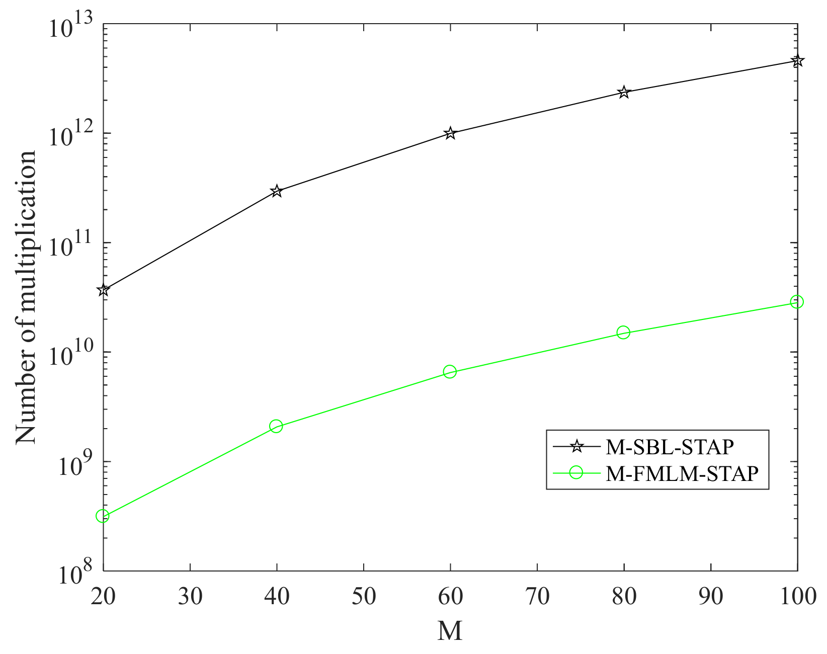
5.1. Complexity Analysis
5.2. Convergence Analysis
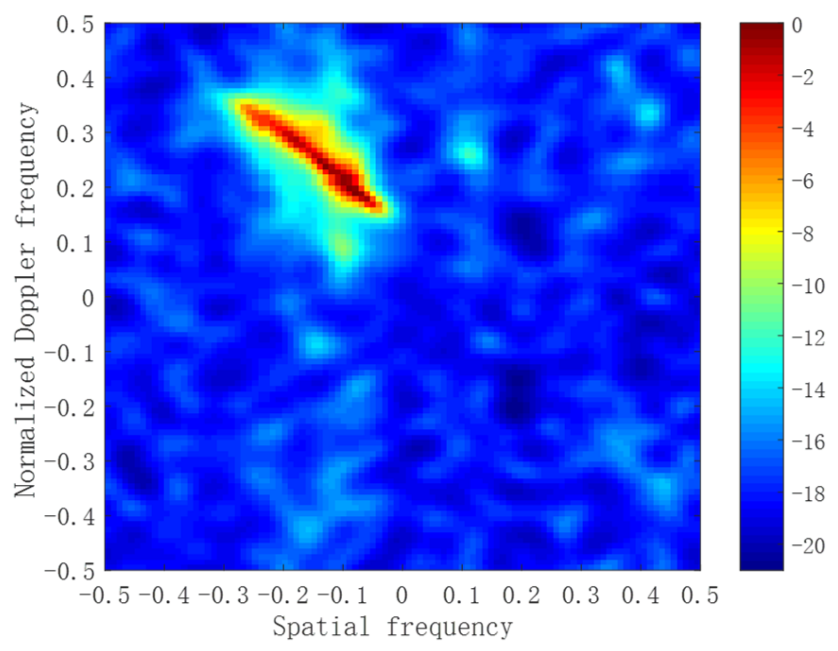
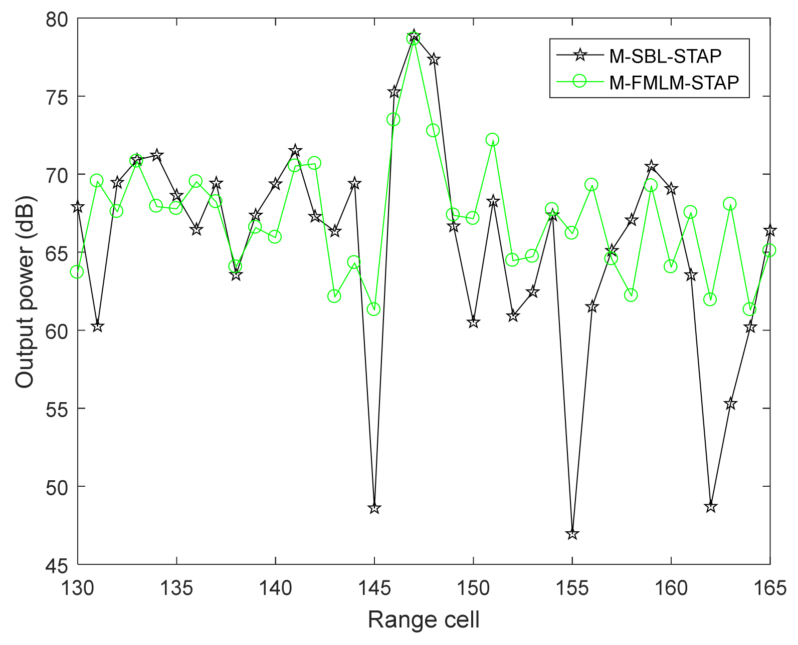
6. Performance Assessment
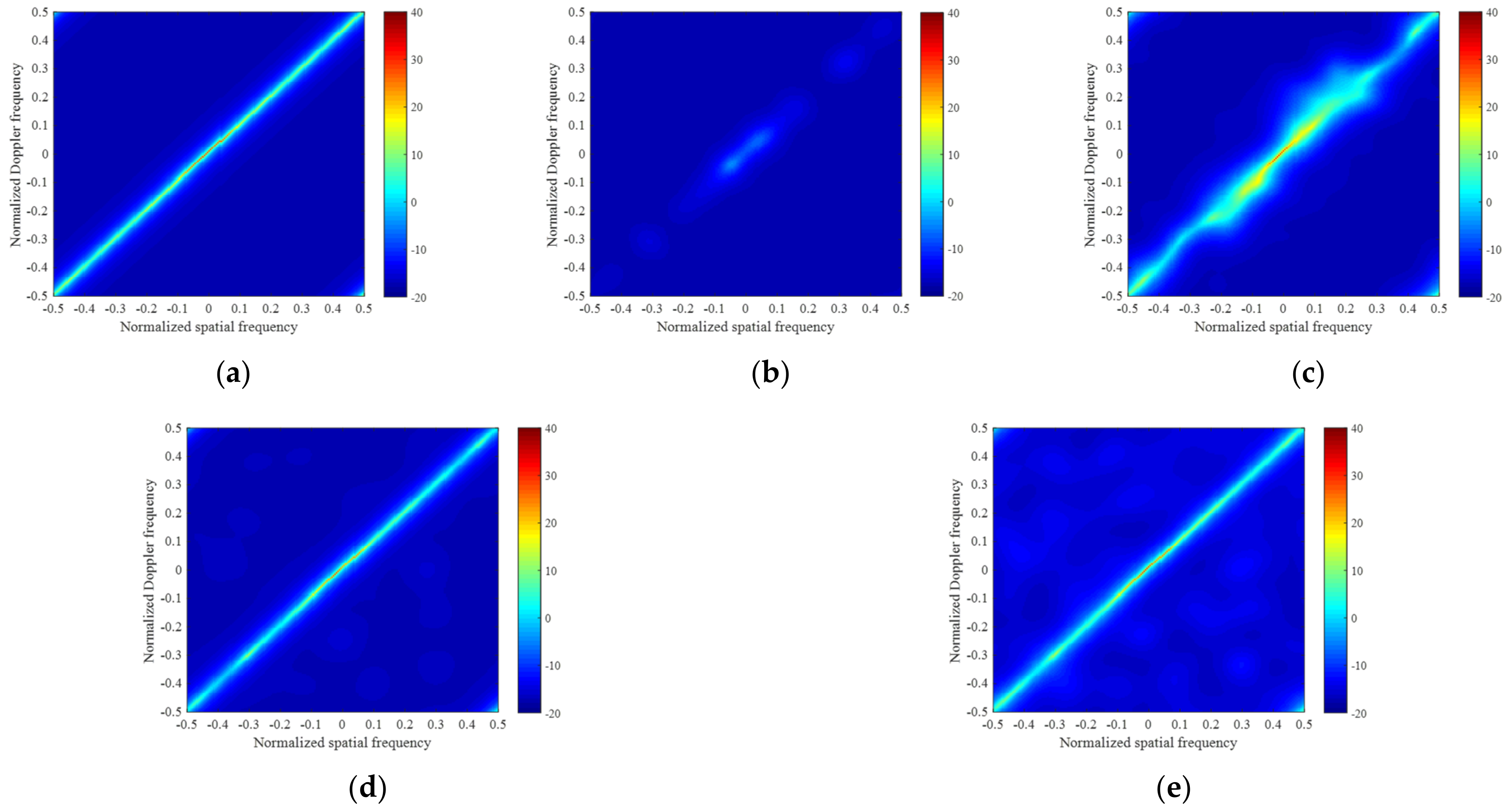
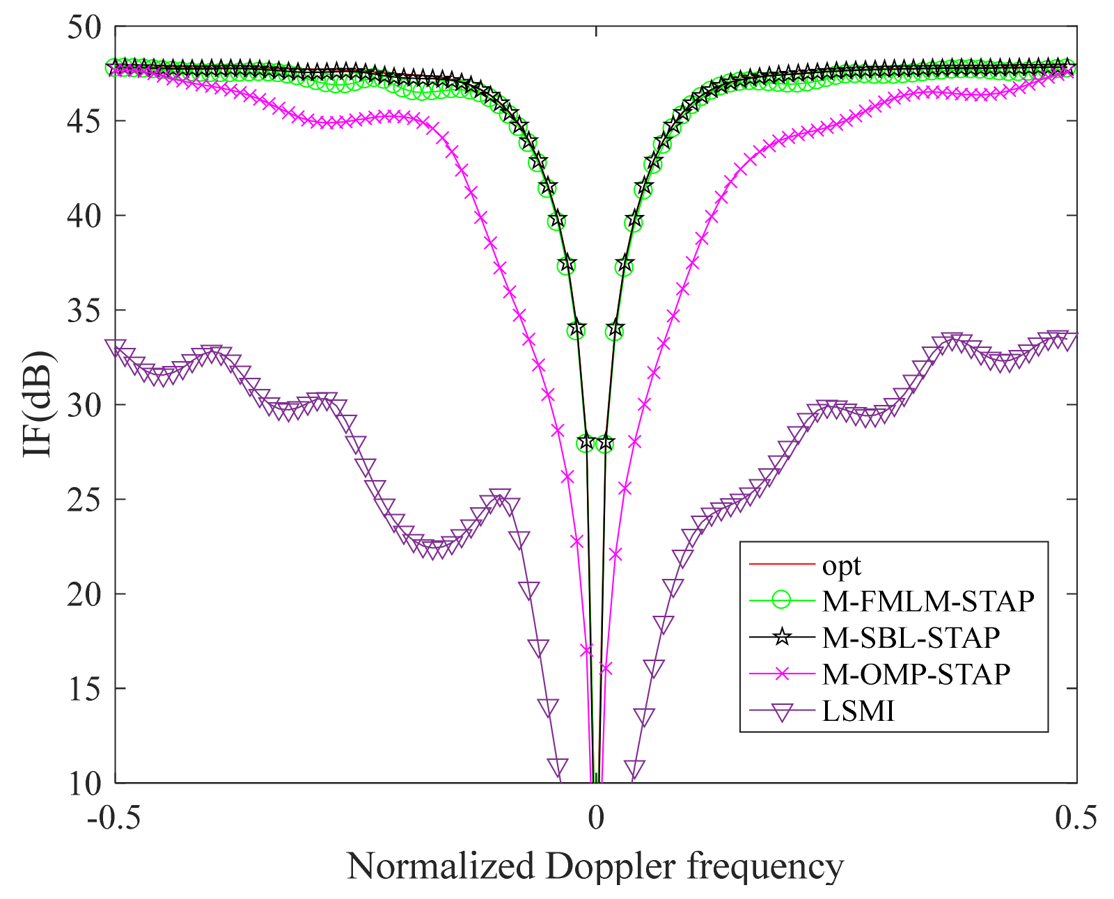
6.1. Simulated Data
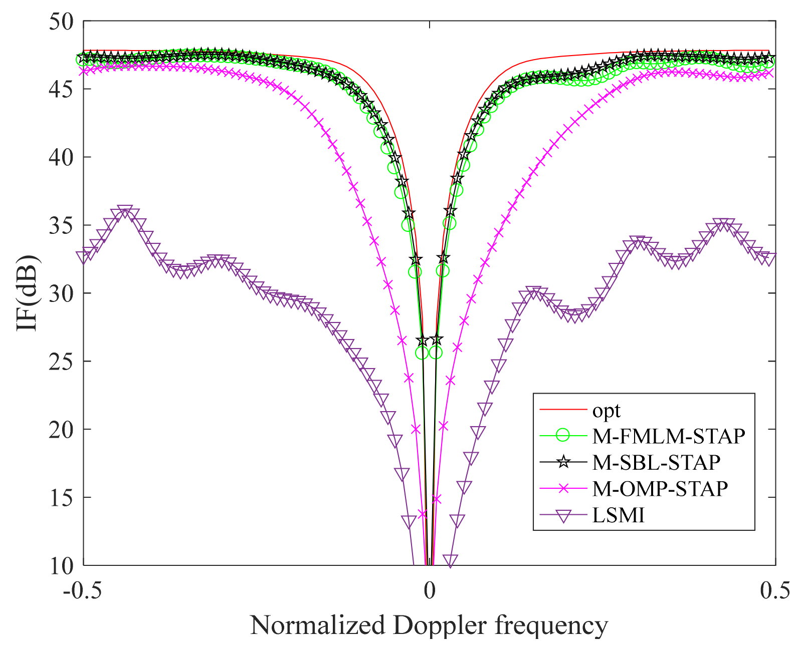
6.2. Measured Data
7. Conclusions
Author Contributions
Funding
Institutional Review Board Statement
Informed Consent Statement
Conflicts of Interest
Appendix A
Appendix A.1. Adding a New Basis Group Function ()
Appendix A.2. Re-Estimating a Basis Group Function ()
Appendix A.3. Deleting a Basis Group Function ()
References
- Ward, J. Space-Time Adaptive Processing for Airborne Radar; Technical Report; MIT Lincoln Laboratory: Lexington, KY, USA, 1998. [Google Scholar]
- Reed, I.S.; Mallet, J.D.; Brennan, L.E. Rapid convergence rate in adaptive arrays. IEEE Trans. Aerosp. Electron. Syst. 1974, AES-10, 853–863. [Google Scholar] [CrossRef]
- Dipietro, R.C. Extended factored space-time processing for airborne radar systems. In Proceedings of the 26th Asilomar Conference on Signals, Systems and Computing, Pacific Grove, CA, USA, 26–28 October 1992; pp. 425–430. [Google Scholar]
- Haimovich, A. The eigencanceler: Adaptive radar by eigenanalysis methods. IEEE Trans. Aerosp. Electron. Syst. 1996, 32, 532–542. [Google Scholar] [CrossRef]
- Melvin, W.L. A STAP overview. IEEE Aerosp. Electron. Syst. Mag. 2004, 19, 19–35. [Google Scholar] [CrossRef]
- Sarkar, T.K.; Park, S.; Koh, J. A deterministic least squares approach to space time adaptive processing. Digit. Signal Process. 1996, 6, 185–194. [Google Scholar] [CrossRef] [Green Version]
- Capraro, C.T.; Capraro, G.T.; Bradaric, I.; Weiner, D.D.; Wicks, M.C.; Baldygo, W.J. Implementing digital terrain data in knowledge-aided space-time adaptive processing. IEEE Trans. Aerosp. Electron. Syst. 2006, 42, 1080–1097. [Google Scholar] [CrossRef]
- Capraro, C.T.; Capraro, G.T.; Weiner, D.D.; Wicks, M.C.; Baldygo, W.J. Improved STAP performance using knowledge-aided secondary data selection. In Proceedings of the 2004 IEEE Radar Conference, Philadelphia, PA, USA, 29 April 2004. [Google Scholar]
- Melvin, W.; Wicks, M.; Antonik, P.; Salama, Y.; Li, P.; Schuman, H. Knowledge-based space-time adaptive processing for airborne early warning radar. IEEE Aerosp. Electron. Syst. Mag. 1998, 13, 37–42. [Google Scholar] [CrossRef]
- Bergin, J.S.; Teixeira, C.M.; Techau, P.M. Improved clutter mitigation performance using knowledge-aided space-time adaptive processing. IEEE Trans. Aerosp. Electron. Syst. 2006, 42, 997–1009. [Google Scholar] [CrossRef]
- Donoho, D.L.; Elad, M.; Temlyakov, V.N. Stable recovery of sparse overcomplete representations in the presence of noise. IEEE Trans. Inf. Theory 2006, 52, 6–18. [Google Scholar] [CrossRef]
- Sun, K.; Zhang, H.; Li, G.; Meng, H.D.; Wang, X.Q. A novel STAP algorithm using sparse recovery technique. In Proceedings of the IEEE International Geoscience and Remote Sensing Symposium, Cape Town, South Africa, 12–17 July 2009; Volume 1, pp. 3761–3764. [Google Scholar]
- Yang, Z.C.; Li, X.; Wang, H.Q.; Jiang, W.D. On clutter sparsity analysis in space-time adaptive processing airborne radar. IEEE Geosci. Remote Sens. Lett. 2013, 10, 1214–1218. [Google Scholar] [CrossRef]
- Yang, Z.C.; de Lamare, R.C.; Li, X. L1-regularized STAP algorithm with a generalized sidelobe canceler architecture for airborne radar. IEEE Trans. Signal Process. 2012, 60, 674–686. [Google Scholar] [CrossRef]
- Sen, S. Low-rank matrix decomposition and spatio-temporal sparse recovery for STAP radar. IEEE J. Sel. Top. Signal Process. 2015, 9, 1510–1523. [Google Scholar] [CrossRef]
- Tipping, M.E. Sparse Bayesian learning and the relevance vector machine. J. Mach. Learn. 2001, 1, 211–244. [Google Scholar]
- Wipf, D.P.; Rao, B.D. Sparse Bayesian learning for basis selection. IEEE Trans. Signal Process. 2004, 52, 2153–2164. [Google Scholar] [CrossRef]
- Wipf, D.P.; Rao, B.D. An empirical Bayesian strategy for solving the simultaneous sparse approximation problem. IEEE Trans. Signal Process. 2007, 55, 3704–3716. [Google Scholar] [CrossRef]
- Tipping, M.E.; Faul, A.C. Fast marginal likelihood maximization for sparse Bayesian models. In Proceedings of the Ninth International Workshop on Artificial Intelligence and Statistics, Key West, FL, USA, 3–6 January 2003; pp. 3–6. [Google Scholar]
- Ji, S.H.; Xue, Y.; Carin, L. Bayesian compressive sensing. IEEE Trans. Signal Process. 2008, 56, 2346–2356. [Google Scholar] [CrossRef]
- Ji, S.H.; Dunson, D.; Carin, L. Multi-task compressive sensing. IEEE Trans. Signal Process. 2009, 57, 92–106. [Google Scholar] [CrossRef]
- Wu, Q.S.; Zhang, Y.M.; Amin, M.G.; Himed, B. Complex multitask Bayesian compressive sensing. In Proceedings of the 2014 IEEE International Conference on Acoustic, Speech and Signal Processing, Florence, Italy, 4–9 May 2014. [Google Scholar]
- Serra, J.G.; Testa, M.; Katsaggelos, A.K. Bayesian K-SVD using fast variational inference. IEEE Trans. Image Process. 2017, 26, 3344–3359. [Google Scholar] [CrossRef]
- Ma, Z.Q.; Dai, W.; Liu, Y.M.; Wang, X.Q. Group sparse Bayesian learning via exact and fast marginal likelihood maximization. IEEE Trans. Signal Process. 2017, 65, 2741–2753. [Google Scholar] [CrossRef]
- Duan, K.Q.; Wang, Z.T.; Xie, W.C.; Chen, H.; Wang, Y.L. Sparsity-based STAP algorithm with multiple measurement vectors via sparse Bayesian learning strategy for airborne radar. IET Signal Process. 2017, 11, 544–553. [Google Scholar] [CrossRef]
- Wang, Z.T.; Xie, W.C.; Duan, K.Q. Clutter suppression algorithm base on fast converging sparse Bayesian learning for airborne radar. Signal Process. 2017, 130, 159–168. [Google Scholar] [CrossRef]
- Yuan, H.D.; Xu, H.; Duan, K.Q.; Xie, W.C.; Liu, W.J.; Wang, Y.L. Sparse Bayesian learning-based space-time adaptive processing with off-grid self-calibration for airborne radar. IEEE Access 2018, 6, 47296–47307. [Google Scholar] [CrossRef]
- Yang, X.P.; Sun, Y.Z.; Yang, J.; Long, T.; Sarkar, T.K. Discrete Interference suppression method based on robust sparse Bayesian learning for STAP. IEEE Access 2019, 10, 26740–26751. [Google Scholar] [CrossRef]
- Bai, Z.L.; Shi, L.M.; Sun, J.W.; Christensen, M.G. Complex sparse signal recovery with adaptive Laplace priors. arXiv 2006, arXiv:2006.16720v1. [Google Scholar]
- Babacan, S.D.; Molina, R.; Katsaggelos, A.K. Bayesian compressive sensing using Laplace priors. IEEE Trans. Image Process. 2010, 19, 53–63. [Google Scholar] [CrossRef]
- Wipf, D.; Nagarajan, S. A new view of automatic relevance determination. Adv. Neural Inf. Process. Syst. 2008, 20, 1–9. [Google Scholar]
- Tropp, J.A. Algorithms for simultaneous sparse approximation, part I: Greedy pursuit. Signal Process. 2006, 86, 572–588. [Google Scholar] [CrossRef]
- Titi, G.W.; Marshall, D.F. The ARPA/NAVY mountaintop program: Adaptive signal processing for airborne early warning radar. In Proceedings of the 1996 IEEE International Conference on Acoustics, Speech, and Signal Processing, Atlanta, GA, USA, 9 May 1996. [Google Scholar]


| Symbols | Parameters | Symbols | Parameters |
|---|---|---|---|
| The original data | The new data | ||
| The original dictionary | The new dictionary | ||
| The original coefficient matrix | The new coefficient matrix | ||
| The original hyper-parameter | The new hyper-parameter | ||
| The covariance of coefficient | The mean of coefficient | ||
| The set of the non-zero values in | The support space of data | ||
| See (54) | See (68) | ||
| See (49) |
| Symbols | Parameters | Value |
|---|---|---|
| Wavelength | 0.3 m | |
| Distance between elements | 0.15 m | |
| Platform velocity | 150 m/s | |
| Platform height | 9000 m | |
| Number of pulses | 8 | |
| Number of channels | 8 | |
| Pulse repetition frequency | 2000 Hz | |
| Range sampling frequency | 2.5 MHz | |
| Perspective angle | 90° | |
| Clutter to noise ratio | 30 dB |
Publisher’s Note: MDPI stays neutral with regard to jurisdictional claims in published maps and institutional affiliations. |
© 2022 by the authors. Licensee MDPI, Basel, Switzerland. This article is an open access article distributed under the terms and conditions of the Creative Commons Attribution (CC BY) license (https://creativecommons.org/licenses/by/4.0/).
Share and Cite
Liu, C.; Wang, T.; Zhang, S.; Ren, B. A Fast Space-Time Adaptive Processing Algorithm Based on Sparse Bayesian Learning for Airborne Radar. Sensors 2022, 22, 2664. https://doi.org/10.3390/s22072664
Liu C, Wang T, Zhang S, Ren B. A Fast Space-Time Adaptive Processing Algorithm Based on Sparse Bayesian Learning for Airborne Radar. Sensors. 2022; 22(7):2664. https://doi.org/10.3390/s22072664
Chicago/Turabian StyleLiu, Cheng, Tong Wang, Shuguang Zhang, and Bing Ren. 2022. "A Fast Space-Time Adaptive Processing Algorithm Based on Sparse Bayesian Learning for Airborne Radar" Sensors 22, no. 7: 2664. https://doi.org/10.3390/s22072664
APA StyleLiu, C., Wang, T., Zhang, S., & Ren, B. (2022). A Fast Space-Time Adaptive Processing Algorithm Based on Sparse Bayesian Learning for Airborne Radar. Sensors, 22(7), 2664. https://doi.org/10.3390/s22072664