
A Cognitive Sample Consensus Method for the Stitching of Drone-Based Aerial Images Supported by a Generative Adversarial Network for False Positive Reduction


Abstract
:1. Introduction
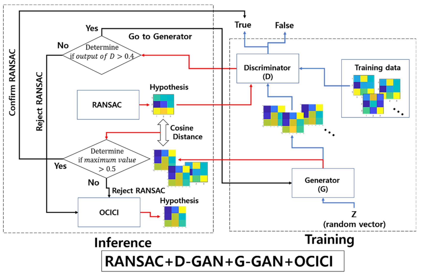
2. Method Description
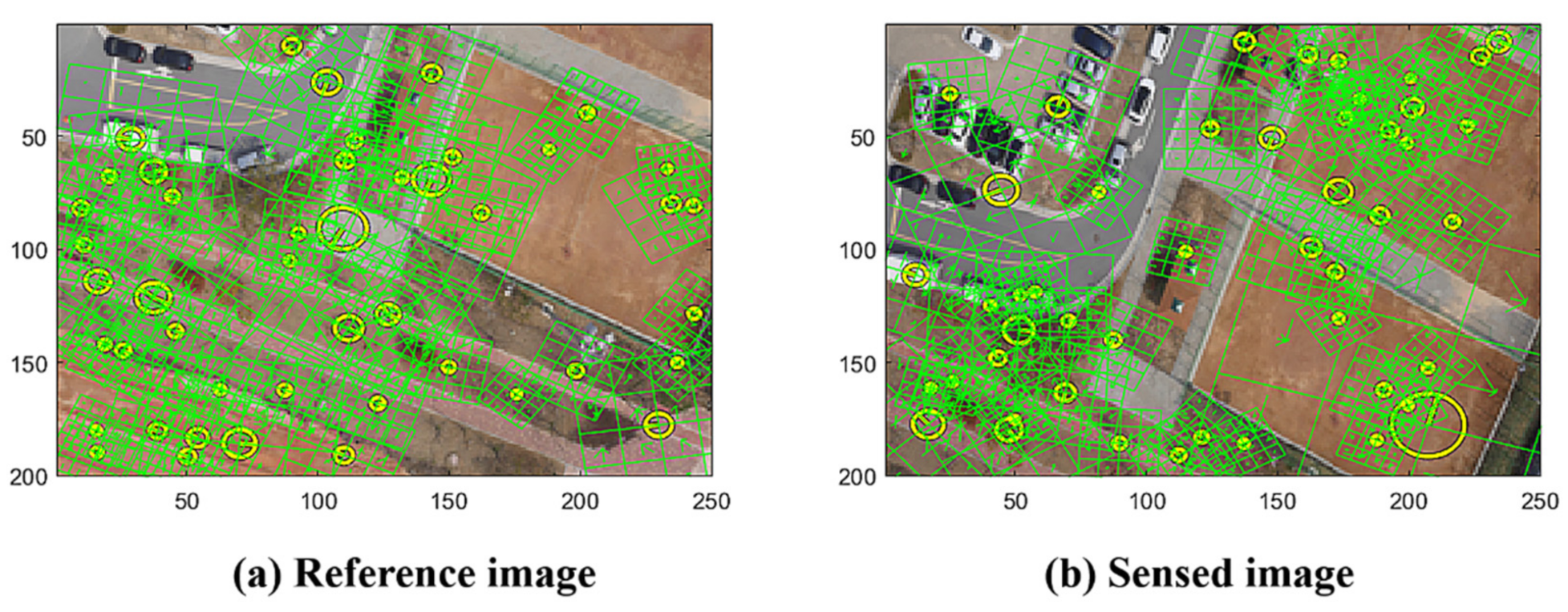
2.1. Extraction of Local Descriptors and Geometric Correspondence
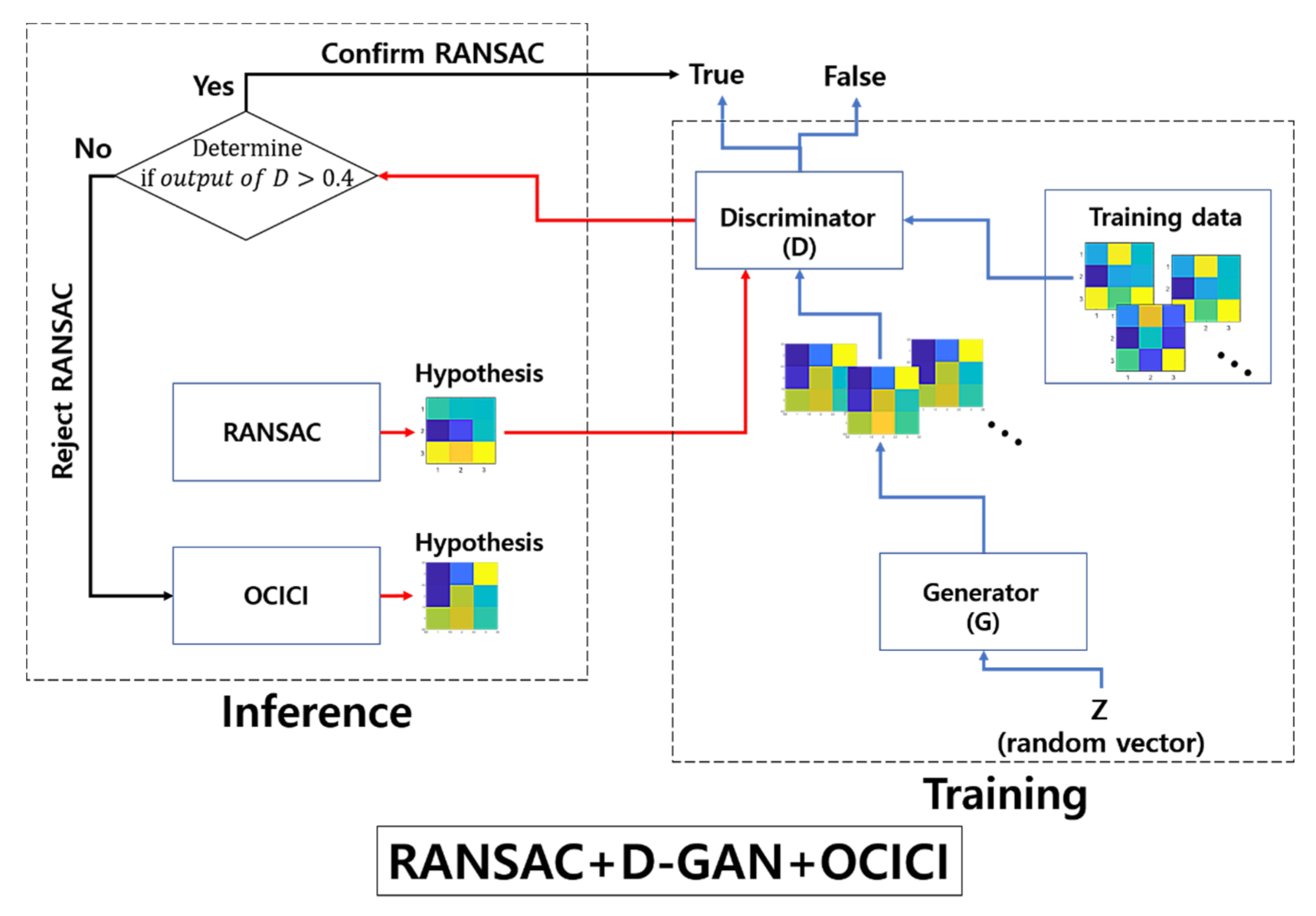
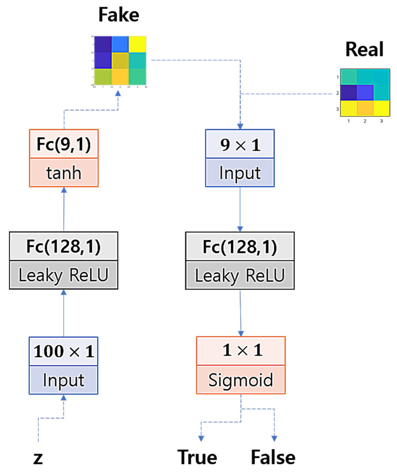
2.2. Outlier Discrimination Network
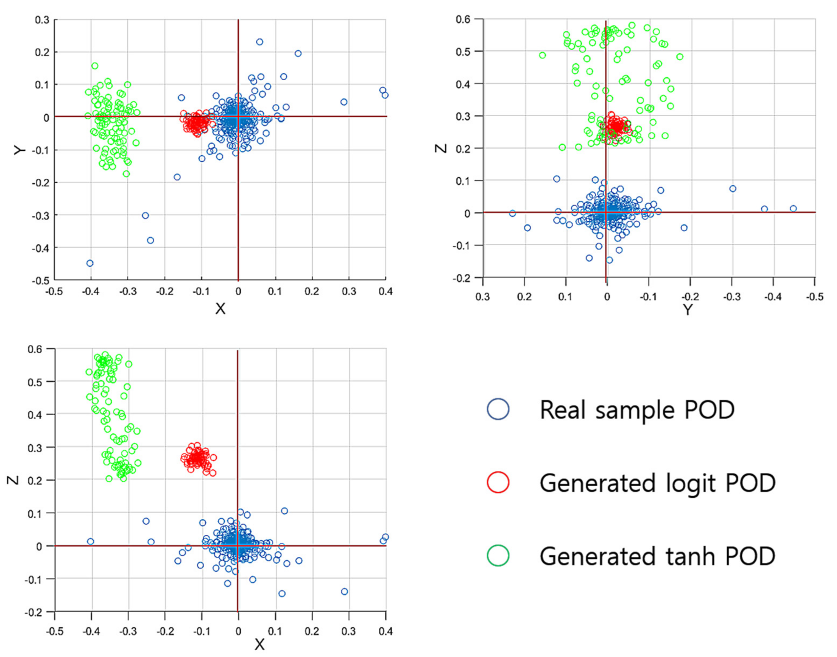
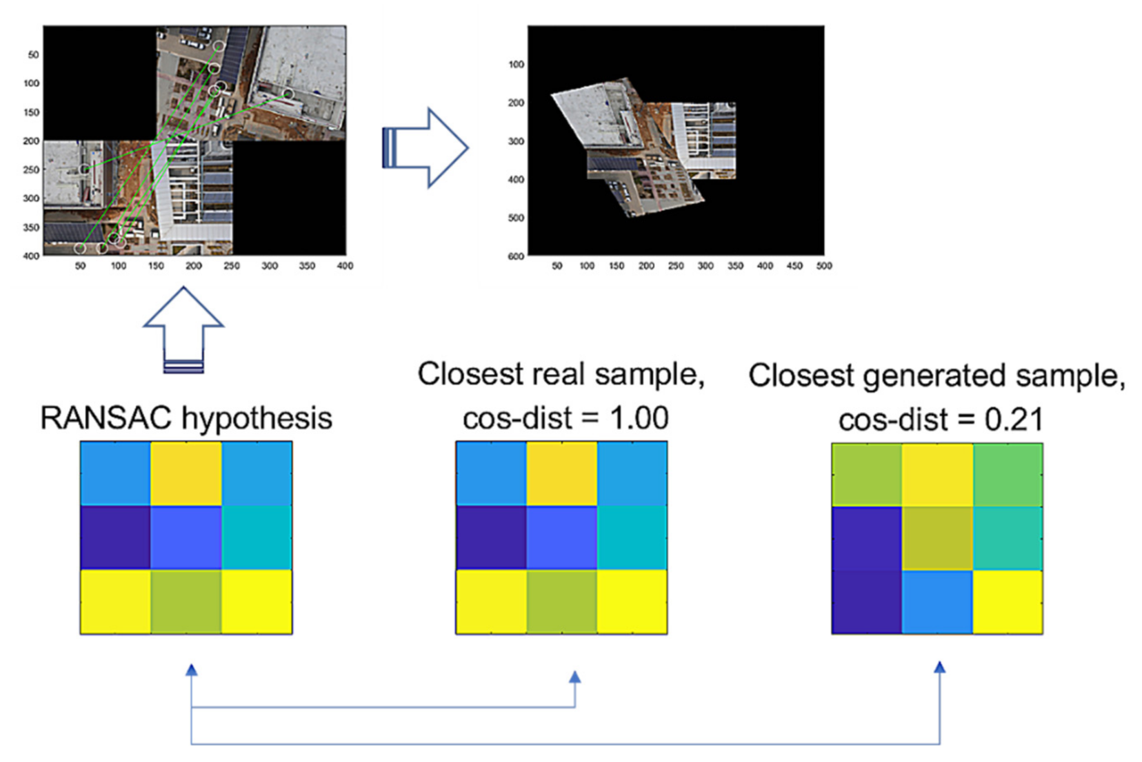
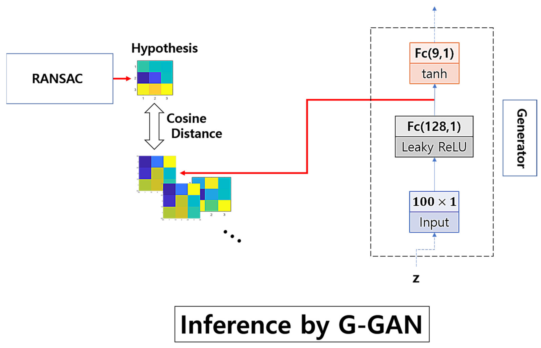
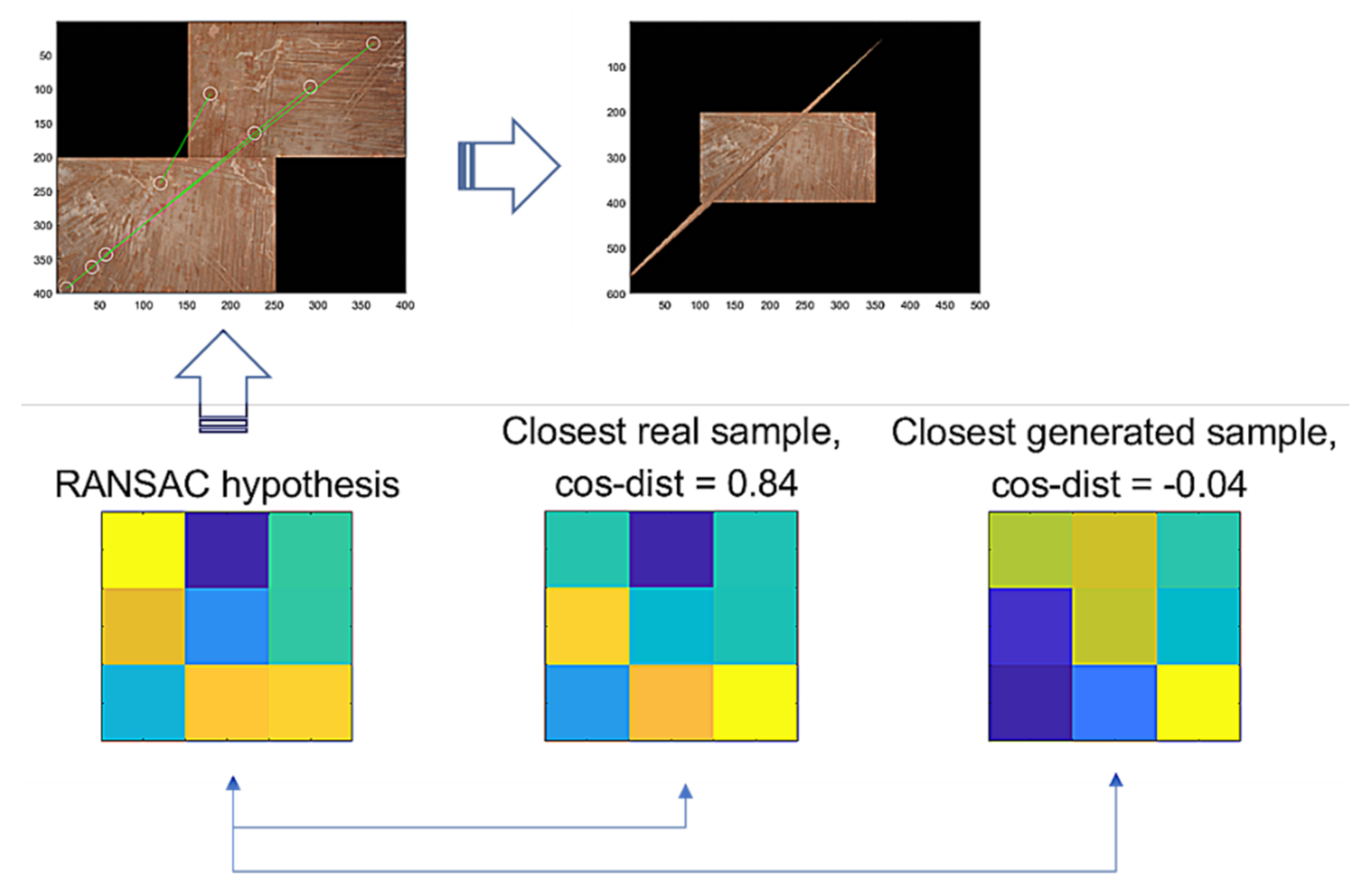
2.3. Generative Comparison Network
3. Results and Analysis
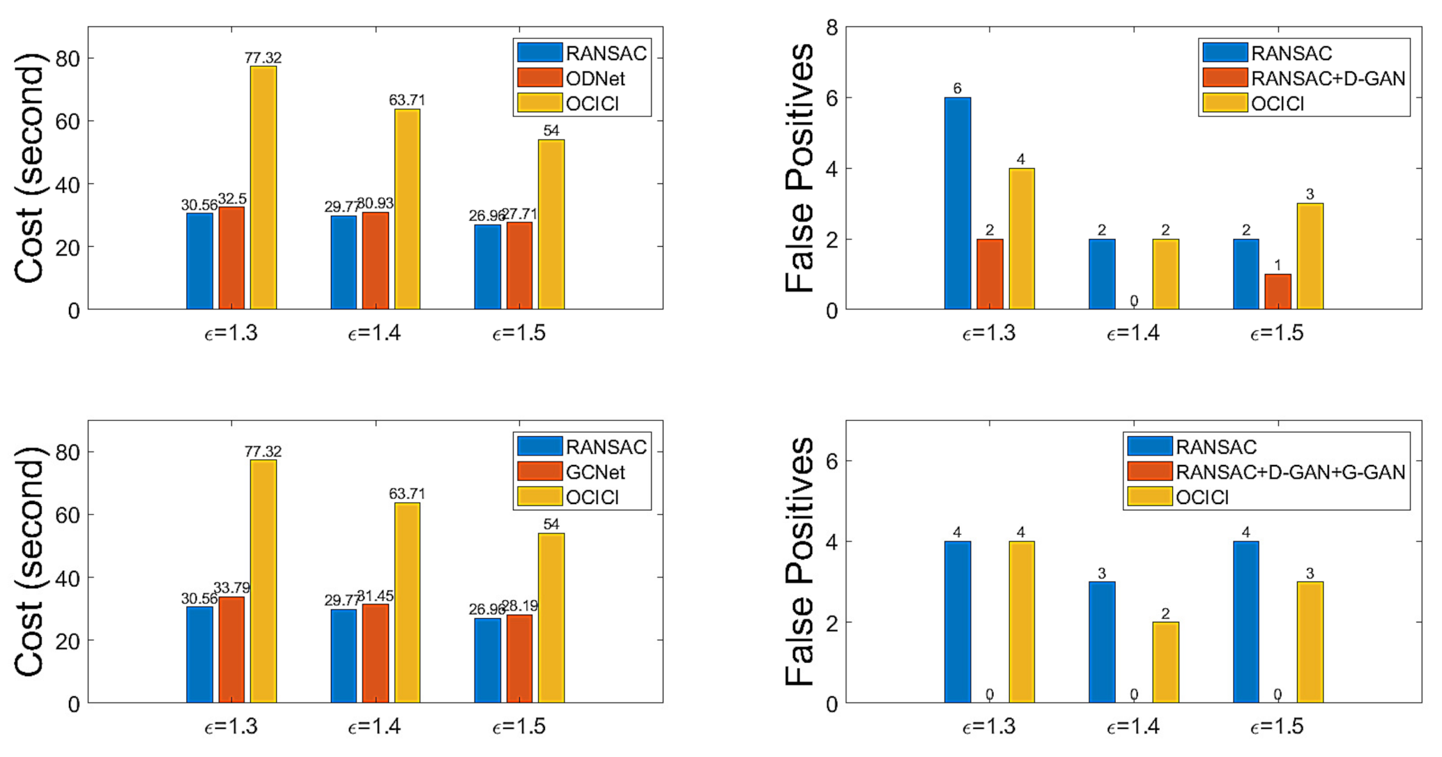
3.1. Experimental Result Applying ODNet
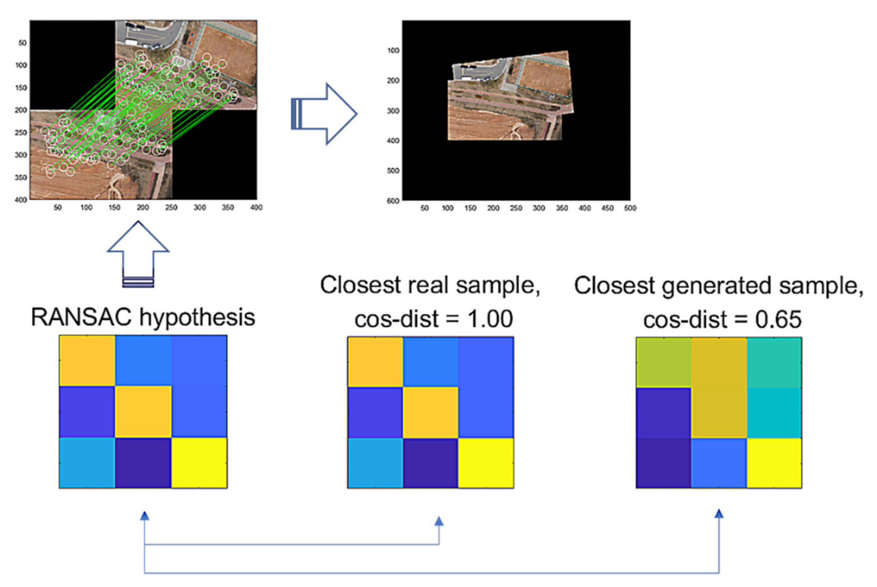
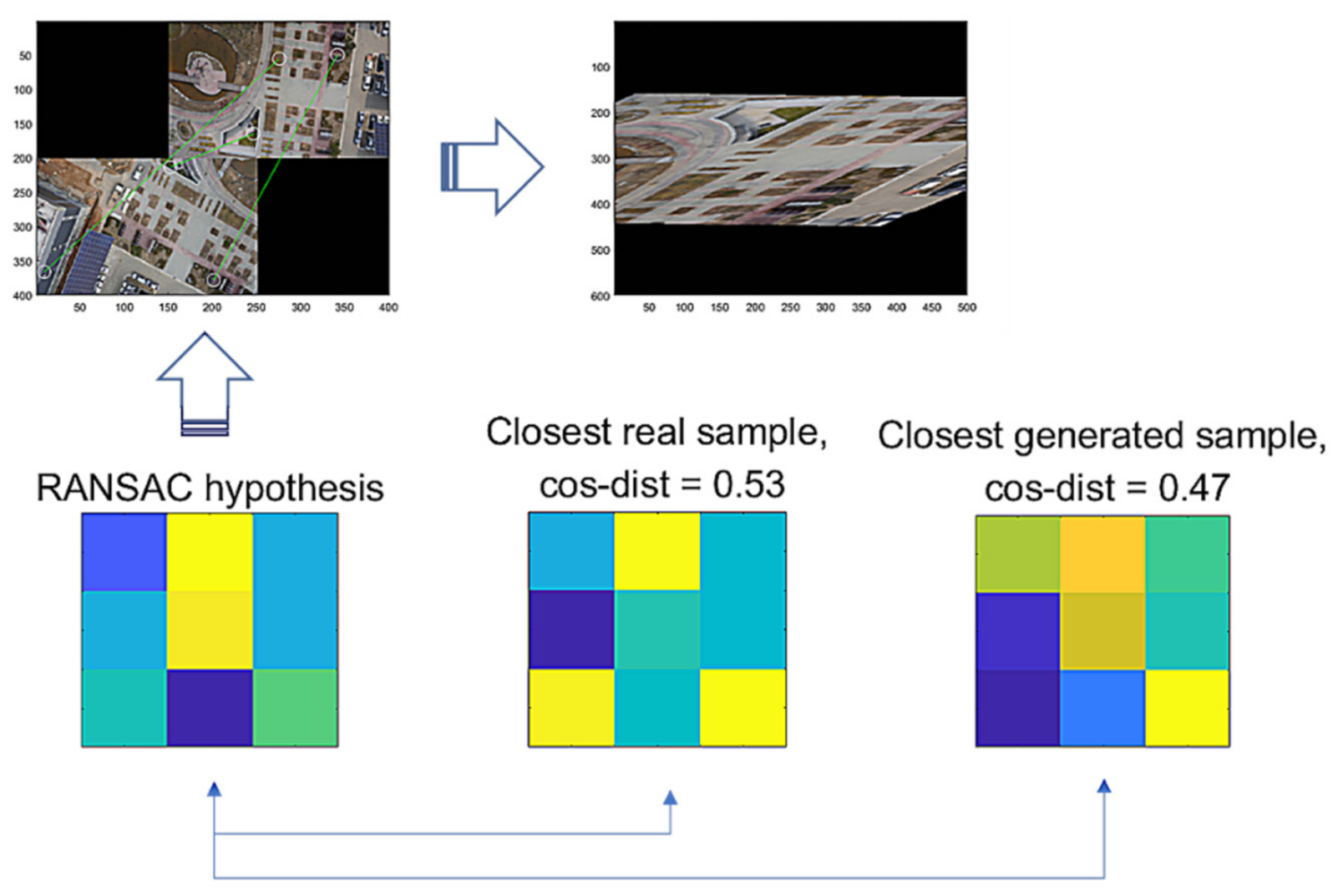
3.2. Experimental Result Applying GCNet
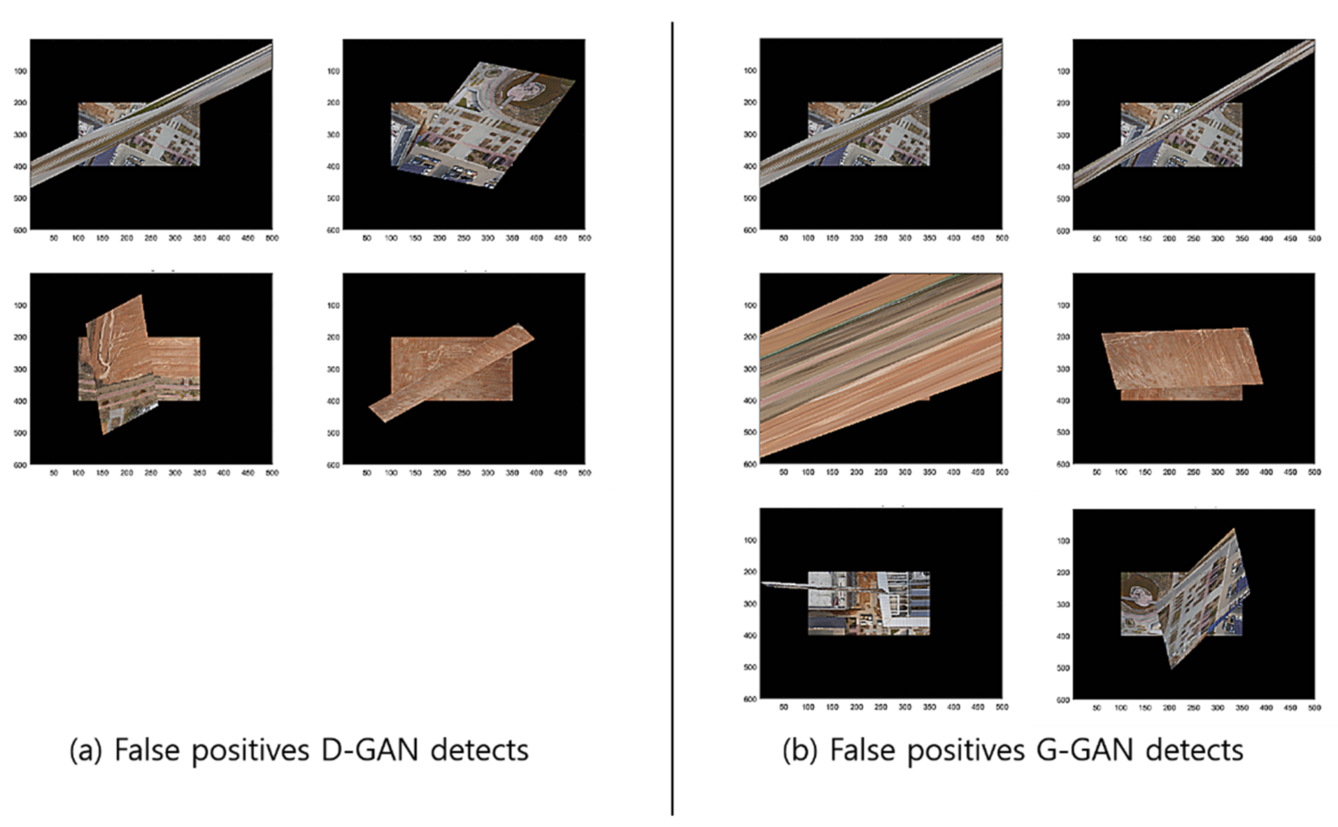
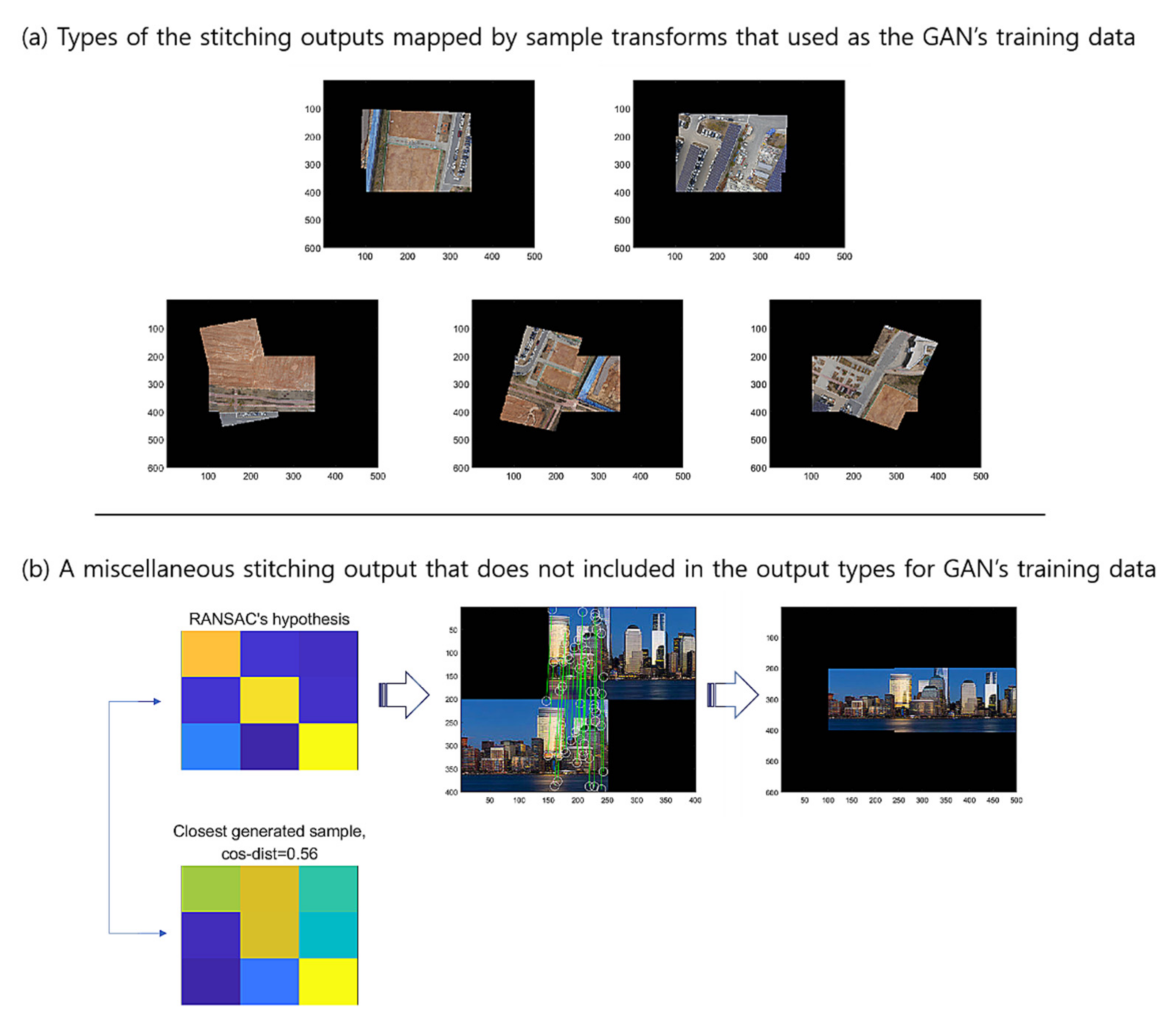
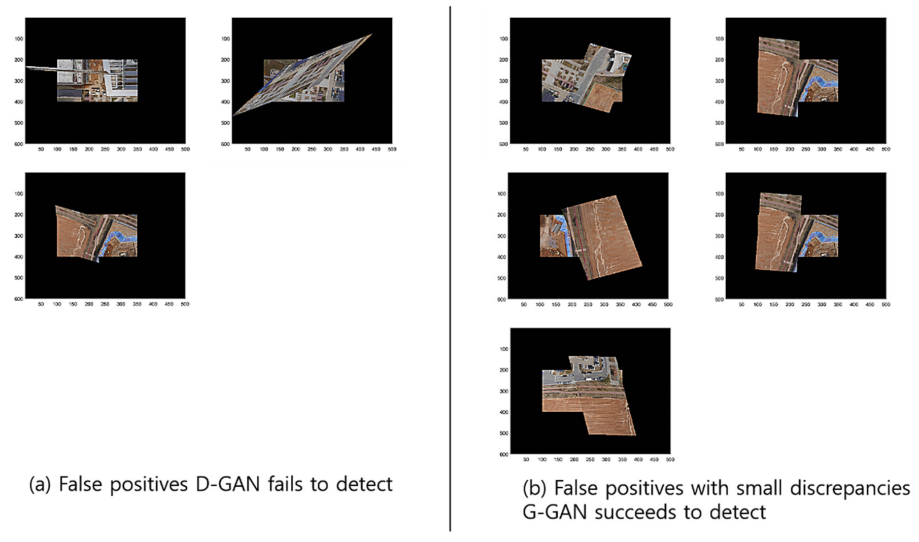
3.3. Discussion and Experiments for Some Miscellaneous Images
4. Conclusions
Funding
Institutional Review Board Statement
Informed Consent Statement
Data Availability Statement
Acknowledgments
Conflicts of Interest
References
- Zitová, B.; Flusser, J. Image registration methods: A survey. Image Vis. Comput. 2003, 21, 977–1000. [Google Scholar] [CrossRef] [Green Version]
- Szeliski, R. Image Alignment and Stitching: A Tutorial. Found. Trends Comput. Graph. Vis. 2006, 2, 1–104. [Google Scholar] [CrossRef]
- Lucas, B.D.; Kanade, T. An iterative image registration technique with an application in stereo vision. In Proceedings of the 7th International Joint Conference on Artificial Intelligence (IJCAI-81), Vancouver, BC, Canada, 24–28 August 1981; pp. 674–679. [Google Scholar]
- Shin, B.-C.; Seo, J.-K. Experimental Optimal Choice Of Initial Candidate Inliers Of The Feature Pairs With Well-Ordering Property For The Sample Consensus Method In The Stitching Of Drone-based Aerial Images. KSII Trans. Internet Inf. Syst. 2020, 14, 1648–1672. [Google Scholar]
- Mundy, J.L. Object Recognition in the Geometric Era: A Retrospective. In Toward Category-Level Object Recognition (LNCS 4170); Springer: New York, NY, USA, 2006; pp. 3–29. [Google Scholar]
- Fu, Y.; Guo, G.; Huang, T.S. Age Synthesis and Estimation via Faces: A Survey. IEEE Trans. Pattern Anal. Mach. Intell. 2010, 32, 1955–1976. [Google Scholar] [PubMed]
- Ng, C.B.; Tay, Y.H.; Goi, B.M. Vision-based human gender recognition: A survey. arXiv 2012, arXiv:1204.1611. [Google Scholar]
- Brox, T.; Malik, J. Large Displacement Optical Flow: Descriptor Matching in Variational Motion Estimation. IEEE Trans. Pattern Anal. Mach. Intell. 2011, 33, 500–513. [Google Scholar] [CrossRef] [PubMed]
- Han, J.; Shao, L.; Xu, D.; Shotton, J. Enhanced Computer Vision With Microsoft Kinect Sensor: A Review. IEEE Trans. Cybern. 2013, 43, 1318–1334. [Google Scholar] [PubMed]
- Shan, C.; Gong, S.; McOwan, P.W. Facial expression recognition based on Local Binary Patterns: A comprehensive study. Image Vis. Comput. 2009, 27, 803–816. [Google Scholar] [CrossRef] [Green Version]
- Kumar, N.; Belhumeur, P.N.; Biswas, A.; Jacobs, D.W.; Kress, W.J.; Lopez, I.C.; Soares, J.V. Leafsnap: A Computer Vision System for Automatic Plant Species Identification. In European Conference on Computer Vision; Springer: Berlin/Heidelberg, Germany, 2012; pp. 502–516. [Google Scholar]
- Oliva, A.; Torralba, A. Chapter 2 Building the gist of a scene: The role of global image features in recognition. In Progress in Brain Research; Elsevier: Amsterdam, The Netherlands, 2006; Volume 155, pp. 23–36. [Google Scholar]
- Weinzaepfel, P.; Revaud, J.; Harchaoui, Z.; Schmid, C. DeepFlow: Large displacement optical flow with deep matching. In Proceedings of the IEEE International Conference on Computer Vision, Sydney, Australia, 2–8 December 2013; pp. 1385–1392. [Google Scholar]
- Lowe, D.G. Distinctive Image Features from Scale-Invariant Keypoints. Int. J. Comput. Vis. 2004, 60, 91–110. [Google Scholar] [CrossRef]
- DeTone, D.; Malisiewicz, T.; Rabinovich, A. Deep image homography estimation. arXiv 2016, arXiv:1606.03798. [Google Scholar]
- Rocco, I.; Arandjelovic, R.; Sivic, J. Convolutional Neural Network Architecture for Geometric Matching. In Proceedings of the 2017 IEEE Conference on Computer Vision and Pattern Recognition (CVPR 2017), Honolulu, HI, USA, 21 July 2017. [Google Scholar]
- Simonyan, K.; Zisserman, A. Very deep convolutional networks for large-scale image recognition. In Proceedings of the International Conference on Learning Representations, ICLR 2015, San Diego, CA, USA, 7–9 May 2015. [Google Scholar]
- Nguyen, T.; Chen, S.W.; Shivakumar, S.S.; Taylor, C.J.; Kumar, V. Unsupervised Deep Homography: A Fast and Robust Homography Estimation Model. IEEE Robot. Autom. Lett. 2018, 3, 2346–2353. [Google Scholar] [CrossRef] [Green Version]
- Fischler, M.A.; Bolles, R.C. Random Sample Consensus: A Paradigm for Model Fitting with Applications to Image Analysis and Automated Cartography. Commun. ACM 1981, 24, 381–395. [Google Scholar] [CrossRef]
- Fischer, P.; Dosovitskiy, A.; Brox, T. Descriptor Matching with Convolutional Neural Networks: A Comparison to SIFT. arXiv 2014, arXiv:1405.5769v1. [Google Scholar]
- Rodriguez, M.; Facciolo, G.; von Gioi, R.G.; Muse, P.; Morel, J.-M.; Delon, J. SIFT-AID: Boosting sift with an affine invariant descriptor based on convolutional neural networks. In Proceedings of the 2019 IEEE International Conference on Image Processing (ICIP), Taipei, Taiwan, 22–25 September 2019. [Google Scholar]
- Vidhyalakshmi, M.K.; Poovammal, E.; Bhaskar, V.; Sathyanarayanan, J. Novel Similarity Metric Learning Using Deep Learning and Root SIFT for Person Re-identification. Wirel. Pers. Commun. 2021, 117, 1835–1851. [Google Scholar] [CrossRef]
- Kang, L.; Wei, Y.; Jiang, J.; Xie, Y. Robust Cylindrical Panorama Stitching for Low-Texture Scenes Based on Image Alignment Using Deep Learning and Iterative Optimization. Sensors 2019, 19, 5310. [Google Scholar] [CrossRef] [PubMed] [Green Version]
- Shen, C.; Ji, X.; Miao, C. Real-Time Image Stitching with Convolutional Neural Networks. In Proceedings of the 2019 IEEE International Conference on Real-Time Computing and Robotics (RCAR), Irkutsk, Russia, 4–9 August 2019. [Google Scholar]
- Zhang, J.; Wang, C.; Liu, S.; Jia, L.; Ye, N.; Wang, J.; Zhou, J.; Sun, J. Content-Aware Unsupervised Deep Homography Estimation. In Proceedings of the European Conference on Computer Vision (ECCV), Glasgow, UK, 23–28 August 2020; pp. 653–669. [Google Scholar]
- Shin, B.-C.; Seo, J.-K. A Posteriori Outlier Rejection Approach Owing to the Well-ordering Property of a Sample Consensus Method for the Stitching of Drone-based Thermal Aerial Images. J. Imaging Sci. Technol. 2021, 65, 20504. [Google Scholar] [CrossRef]
- Goodfellow, I.; Pouget-Abadie, J.; Mirza, M.; Xu, B.; Warde-Farley, D.; Ozair, S.; Courville, A.; Bengio, Y. Generative adversarial nets. Adv. Neural Inf. Process. Syst. 2014, 27, 2672–2680. [Google Scholar]
- Zheng, L.; Yang, Y.; Tian, Q. SIFT Meets CNN: A Decade Survey of Instance Retrieval. IEEE Trans. Pattern Anal. Mach. Intell. 2018, 40, 1224–1244. [Google Scholar] [CrossRef] [PubMed] [Green Version]
- Seo, J.-K. DataSet: Remote Sensing-Drone Aerial Images around Photovoltaic Panels (200 by 250 Resolution). 2020. Available online: https://github.com/seojksc/seojk-kuids (accessed on 10 November 2021).
- Goodfellow, I.; Bengio, Y.; Courville, A. Deep Learning; MIT Press: Cambridge, MA, USA, 2017. [Google Scholar]
- Seo, J.-K.; Kim, Y.J.; Kim, K.G.; Shin, I.; Shin, J.H.; Kwak, J.Y. Differentiation of the Follicular Neoplasm on the Gray-Scale US by Image Selection Subsampling along with the Marginal Outline Using Convolutional Neural Network. BioMed Res. Int. 2017, 2017, 3098293. [Google Scholar] [CrossRef] [PubMed] [Green Version]
- Liang, Y.; Lee, H.; Lim, S.; Lin, W.; Lee, K.; Wu, C. Proper orthogonal decomposition and its applications—Part I: Theory. J. Sound Vib. 2002, 252, 527–544. [Google Scholar] [CrossRef]


| C(Logit, T) > C(tanh, T) | (Logit, T) < C(tanh, T) | Total | |
| Number of cases | 15,601 | 777 | 16,378 |
| C(Logit, T) > C(tanh, T) | (Logit, T) < C(tanh, T) | Total | |
|---|---|---|---|
| Number of cases | 15,325 | 1053 | 16,378 |
| Stitching View by RANSAC | False Positive Case vs. Total Cases by RANSAC | False Positive Cases vs. Total Cases by D-GAN | |
|---|---|---|---|
 | 0/20 | 0/20 (False negative rate = 100%) | |
 | 0/20 | 0/20 (False negative rate = 100%) | |
 | 0/20 | 0/20 (True positive rate = 100%) | |
 | 0/20 | 0/20 (True positive rate = 100%) | |
 | 11/20 | 1/20 (True positive cases = 0) | |
 | 0/20 | 0/20 (False negative rate = 100%) | |
| Total false positive rate | 9.1667% | 2.439% | |
| RANSAC | ODNet | OCICI | ||
|---|---|---|---|---|
| Accuracy | 96.8254% | 100% | 100% | |
| 98.4127% | 100% | 100% | ||
| 90.4762% | 93.6508% (max 96.8254%) | 93.6508% | ||
| 96.6102% | 98.3051% (max 100%) | 96.6102% | ||
| 96.5517% | 96.5517% (max 98.2759%) | 94.8276% | ||
| Cost | 34.2061 | 66.6555 | 318.6295 | |
| 89.5633 | 94.3174 | 145.6169 | ||
| 30.5566 | 32.4998 | 77.3177 | ||
| 29.7655 | 30.9285 | 63.7132 | ||
| 26.9586 | 27.7069 | 54.0032 |
| Accuracy | 85.7143% | 85.7143% | 90.4762% | 89.8305% | 89.6552% |
| FP | 0/52 | 0/53 | 2/55 | 0/51 | 1/52 |
| FN | 9/11 | 9/10 | 4/8 | 6/8 | 5/6 |
| TND | 2/2 | 1/1 | 4/6 | 2/2 | 1/2 |
| RANSAC | GCNet | OCICI | ||
|---|---|---|---|---|
| Accuracy | 93.6508% | 93.6508% (max 100%) | 93.6508% | |
| 94.9153% | 96.6102% (max 100%) | 96.6102% | ||
| 93.1034% | 94.8276% (max 100%) | 94.8276% | ||
| Cost | 30.5566 | 33.7912 | 77.3177 | |
| 29.7655 | 31.4479 | 63.7132 | ||
| 26.9586 | 28.1906 | 54.0032 |
| Accuracy | 76.1905% | 79.6610% | 82.7586% |
| FP | 0/44 | 0/44 | 0/44 |
| FN | 15/19 | 12/15 | 10/14 |
| TND | 4/4 | 3/3 | 4/4 |
| Matching Correspondences | False Stitching Output | FP (for 20 Trials) |
|---|---|---|
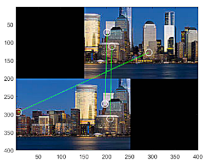 |  | RANSAC: 10% |
| D-GAN: 5% | ||
| G-GAN: 5% | ||
 |  | RANSAC: 40% |
| D-GAN: 15% | ||
| G-GAN: 0% |
Publisher’s Note: MDPI stays neutral with regard to jurisdictional claims in published maps and institutional affiliations. |
© 2022 by the author. Licensee MDPI, Basel, Switzerland. This article is an open access article distributed under the terms and conditions of the Creative Commons Attribution (CC BY) license (https://creativecommons.org/licenses/by/4.0/).
Share and Cite
Seo, J.-K. A Cognitive Sample Consensus Method for the Stitching of Drone-Based Aerial Images Supported by a Generative Adversarial Network for False Positive Reduction. Sensors 2022, 22, 2474. https://doi.org/10.3390/s22072474
Seo J-K. A Cognitive Sample Consensus Method for the Stitching of Drone-Based Aerial Images Supported by a Generative Adversarial Network for False Positive Reduction. Sensors. 2022; 22(7):2474. https://doi.org/10.3390/s22072474
Chicago/Turabian StyleSeo, Jeong-Kweon. 2022. "A Cognitive Sample Consensus Method for the Stitching of Drone-Based Aerial Images Supported by a Generative Adversarial Network for False Positive Reduction" Sensors 22, no. 7: 2474. https://doi.org/10.3390/s22072474
APA StyleSeo, J.-K. (2022). A Cognitive Sample Consensus Method for the Stitching of Drone-Based Aerial Images Supported by a Generative Adversarial Network for False Positive Reduction. Sensors, 22(7), 2474. https://doi.org/10.3390/s22072474