
Data Fusion in Agriculture: Resolving Ambiguities and Closing Data Gaps


Abstract
:1. Introduction
2. Literature Review
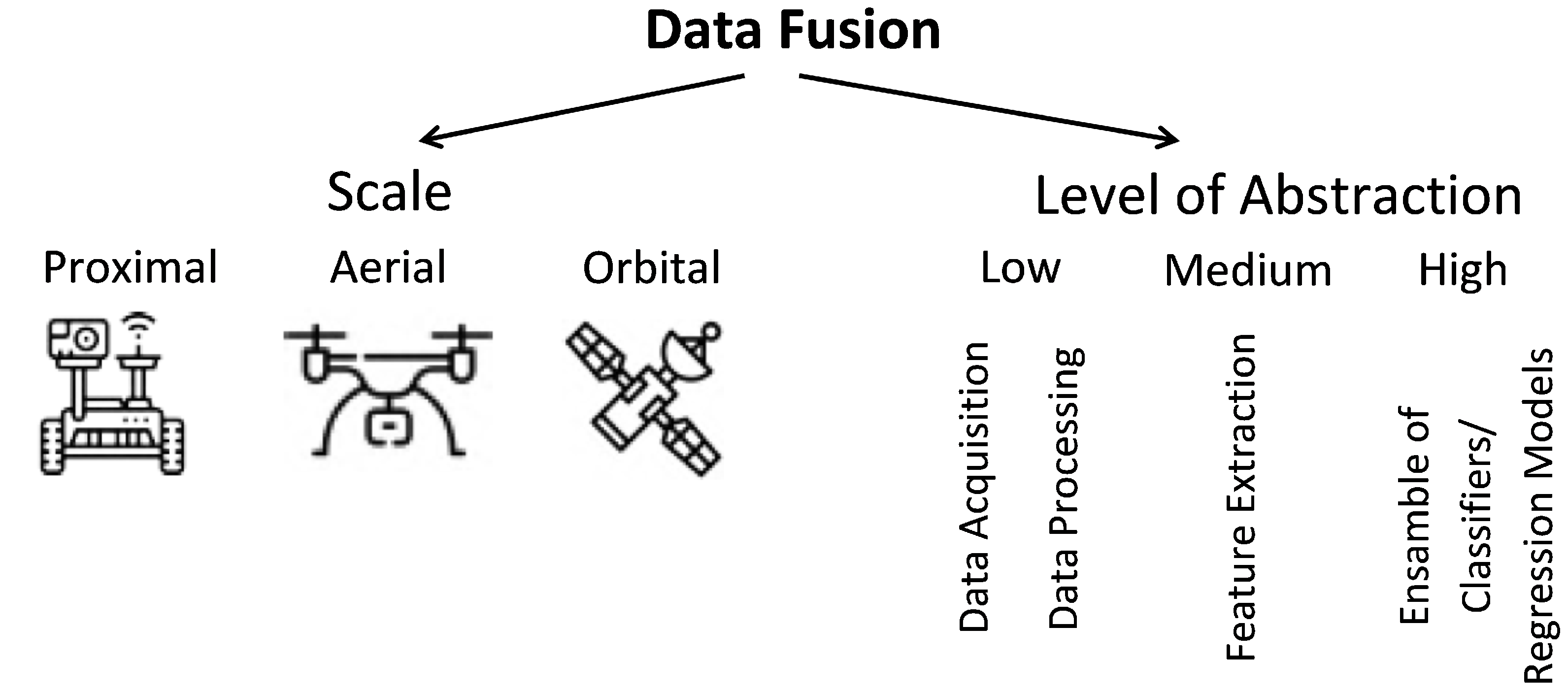
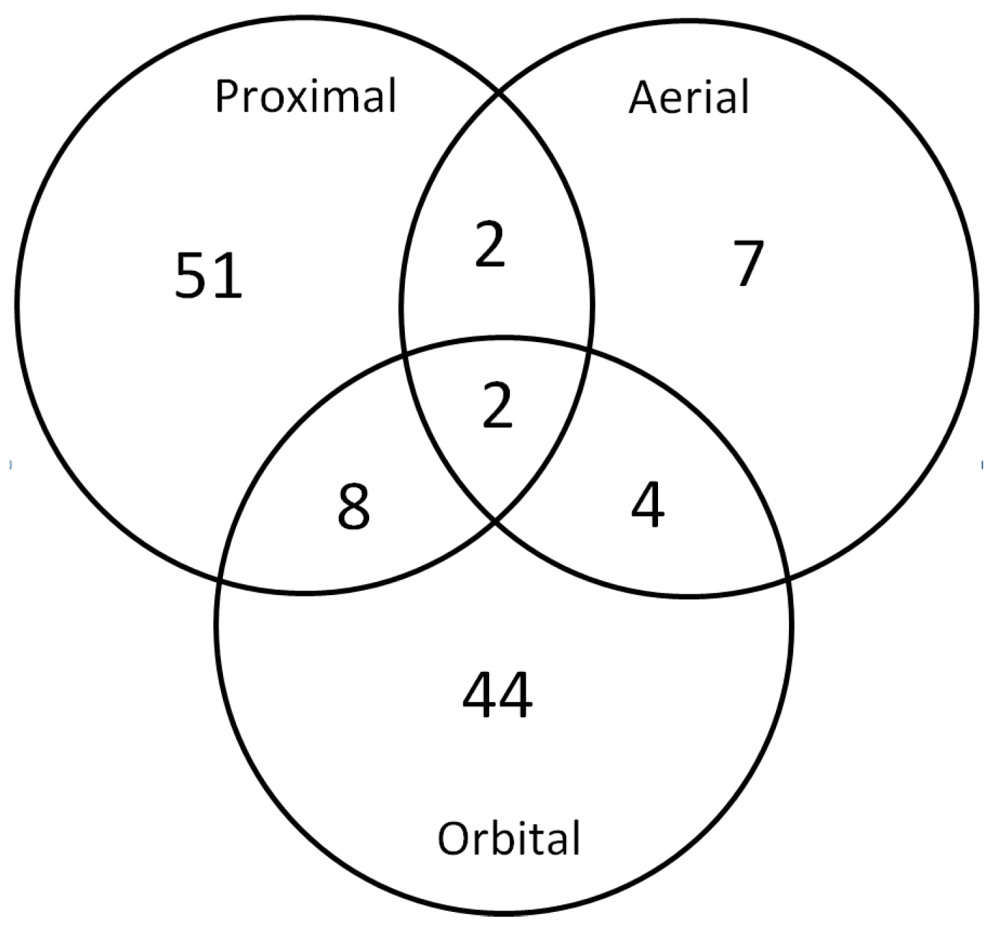
2.1. Proximal Scale
2.2. Aerial Scale
2.3. Orbital Scale
3. Discussion
3.1. Comparison of the Results Yielded by Fused and Individual Sources of Data
3.2. Data Fusion Techniques
3.3. Data Fusion Level
3.4. Differences between Fusion Techniques
3.5. Limitations of Current Studies
3.6. Types of Data
3.7. Other Issues
4. Conclusions
Funding
Institutional Review Board Statement
Informed Consent Statement
Data Availability Statement
Conflicts of Interest
References
- Barbedo, J. Deep learning applied to plant pathology: The problem of data representativeness. Trop. Plant Pathol. 2022, 47, 85–94. [Google Scholar] [CrossRef]
- Kamilaris, A.; Kartakoullis, A.; Prenafeta-Boldú, F.X. A review on the practice of big data analysis in agriculture. Comput. Electron. Agric. 2017, 143, 23–37. [Google Scholar] [CrossRef]
- Coble, K.H.; Mishra, A.K.; Ferrell, S.; Griffin, T. Big Data in Agriculture: A Challenge for the Future. Appl. Econ. Perspect. Policy 2018, 40, 79–96. [Google Scholar] [CrossRef] [Green Version]
- Barbedo, J.G. Factors influencing the use of deep learning for plant disease recognition. Biosyst. Eng. 2018, 172, 84–91. [Google Scholar] [CrossRef]
- Munir, A.; Blasch, E.; Kwon, J.; Kong, J.; Aved, A. Artificial Intelligence and Data Fusion at the Edge. IEEE Aerosp. Electron. Syst. Mag. 2021, 36, 62–78. [Google Scholar] [CrossRef]
- Solberg, A.; Jain, A.; Taxt, T. Multisource classification of remotely sensed data: Fusion of Landsat TM and SAR images. IEEE Trans. Geosci. Remote Sens. 1994, 32, 768–778. [Google Scholar] [CrossRef]
- Bleiholder, J.; Naumann, F. Data Fusion. ACM Comput. Surv. 2009, 41, 1–40. [Google Scholar] [CrossRef]
- Caruccio, L.; Cirillo, S. Incremental Discovery of Imprecise Functional Dependencies. J. Data Inf. Qual. 2020, 12, 1–25. [Google Scholar] [CrossRef]
- Dalla Mura, M.; Prasad, S.; Pacifici, F.; Gamba, P.; Chanussot, J.; Benediktsson, J.A. Challenges and Opportunities of Multimodality and Data Fusion in Remote Sensing. Proc. IEEE 2015, 103, 1585–1601. [Google Scholar] [CrossRef] [Green Version]
- Ouhami, M.; Hafiane, A.; Es-Saady, Y.; El Hajji, M.; Canals, R. Computer Vision, IoT and Data Fusion for Crop Disease Detection Using Machine Learning: A Survey and Ongoing Research. Remote Sens. 2021, 13, 2486. [Google Scholar] [CrossRef]
- Erfani, S.; Jafari, A.; Hajiahmad, A. Comparison of two data fusion methods for localization of wheeled mobile robot in farm conditions. Artif. Intell. Agric. 2019, 1, 48–55. [Google Scholar] [CrossRef]
- Guo, L.; Zhang, Q. Wireless Data Fusion System for Agricultural Vehicle Positioning. Biosyst. Eng. 2005, 91, 261–269. [Google Scholar] [CrossRef]
- Han, J.H.; Park, C.H.; Kwon, J.H.; Lee, J.; Kim, T.S.; Jang, Y.Y. Performance Evaluation of Autonomous Driving Control Algorithm for a Crawler-Type Agricultural Vehicle Based on Low-Cost Multi-Sensor Fusion Positioning. Appl. Sci. 2020, 10, 4667. [Google Scholar] [CrossRef]
- Khot, L.; Tang, L.; Steward, B.; Han, S. Sensor fusion for improving the estimation of roll and pitch for an agricultural sprayer. Biosyst. Eng. 2008, 101, 13–20. [Google Scholar] [CrossRef]
- Li, Y.; Jia, H.; Qi, J.; Sun, H.; Tian, X.; Liu, H.; Fan, X. An Acquisition Method of Agricultural Equipment Roll Angle Based on Multi-Source Information Fusion. Sensors 2020, 20, 2082. [Google Scholar] [CrossRef] [Green Version]
- Zaidner, G.; Shapiro, A. A novel data fusion algorithm for low-cost localisation and navigation of autonomous vineyard sprayer robots. Biosyst. Eng. 2016, 146, 133–148. [Google Scholar] [CrossRef]
- Zhang, Q.; Chen, Q.; Xu, Z.; Zhang, T.; Niu, X. Evaluating the navigation performance of multi-information integration based on low-end inertial sensors for precision agriculture. Precis. Agric. 2021, 22, 627–646. [Google Scholar] [CrossRef]
- Bulanon, D.; Burks, T.; Alchanatis, V. Image fusion of visible and thermal images for fruit detection. Biosyst. Eng. 2009, 103, 12–22. [Google Scholar] [CrossRef]
- Gan, H.; Lee, W.; Alchanatis, V.; Ehsani, R.; Schueller, J. Immature green citrus fruit detection using color and thermal images. Comput. Electron. Agric. 2018, 152, 117–125. [Google Scholar] [CrossRef]
- Li, P.; Lee, S.H.; Hsu, H.Y.; Park, J.S. Nonlinear Fusion of Multispectral Citrus Fruit Image Data with Information Contents. Sensors 2017, 17, 142. [Google Scholar] [CrossRef] [Green Version]
- Sa, I.; Ge, Z.; Dayoub, F.; Upcroft, B.; Perez, T.; McCool, C. DeepFruits: A Fruit Detection System Using Deep Neural Networks. Sensors 2016, 16, 1222. [Google Scholar] [CrossRef] [PubMed] [Green Version]
- Cruz, A.C.; Luvisi, A.; De Bellis, L.; Ampatzidis, Y. X-FIDO: An Effective Application for Detecting Olive Quick Decline Syndrome with Deep Learning and Data Fusion. Front. Plant Sci. 2017, 8, 1741. [Google Scholar] [CrossRef] [PubMed]
- Moshou, D.; Bravo, C.; Oberti, R.; West, J.; Bodria, L.; McCartney, A.; Ramon, H. Plant disease detection based on data fusion of hyper-spectral and multi-spectral fluorescence imaging using Kohonen maps. Real-Time Imaging 2005, 11, 75–83. [Google Scholar] [CrossRef]
- Shankar, P.; Johnen, A.; Liwicki, M. Data Fusion and Artificial Neural Networks for Modelling Crop Disease Severity. In Proceedings of the 2020 IEEE 23rd International Conference on Information Fusion (FUSION), Rustenburg, South Africa, 6–9 July 2020; pp. 1–8. [Google Scholar] [CrossRef]
- Anastasiou, E.; Castrignanò, A.; Arvanitis, K.; Fountas, S. A multi-source data fusion approach to assess spatial-temporal variability and delineate homogeneous zones: A use case in a table grape vineyard in Greece. Sci. Total Environ. 2019, 684, 155–163. [Google Scholar] [CrossRef]
- De Benedetto, D.; Castrignano, A.; Diacono, M.; Rinaldi, M.; Ruggieri, S.; Tamborrino, R. Field partition by proximal and remote sensing data fusion. Biosyst. Eng. 2013, 114, 372–383. [Google Scholar] [CrossRef]
- Castrignanò, A.; Buttafuoco, G.; Quarto, R.; Parisi, D.; Viscarra Rossel, R.; Terribile, F.; Langella, G.; Venezia, A. A geostatistical sensor data fusion approach for delineating homogeneous management zones in Precision Agriculture. CATENA 2018, 167, 293–304. [Google Scholar] [CrossRef]
- Guerrero, A.; De Neve, S.; Mouazen, A.M. Data fusion approach for map-based variable-rate nitrogen fertilization in barley and wheat. Soil Tillage Res. 2021, 205, 104789. [Google Scholar] [CrossRef]
- Shaddad, S.; Madrau, S.; Castrignanò, A.; Mouazen, A. Data fusion techniques for delineation of site-specific management zones in a field in UK. Precis. Agric. 2016, 17, 200–217. [Google Scholar] [CrossRef]
- Afriyie, E.; Verdoodt, A.; Mouazen, A.M. Data fusion of visible near-infrared and mid-infrared spectroscopy for rapid estimation of soil aggregate stability indices. Comput. Electron. Agric. 2021, 187, 106229. [Google Scholar] [CrossRef]
- Casa, R.; Castaldi, F.; Pascucci, S.; Basso, B.; Pignatti, S. Geophysical and Hyperspectral Data Fusion Techniques for In-Field Estimation of Soil Properties. Vadose Zone J. 2013, 12, vzj2012.0201. [Google Scholar] [CrossRef]
- Huo, Z.; Tian, J.; Wu, Y.; Ma, F. A Soil Environmental Quality Assessment Model Based on Data Fusion and Its Application in Hebei Province. Sustainability 2020, 12, 6804. [Google Scholar] [CrossRef]
- Ji, W.; Adamchuk, V.I.; Chen, S.; Mat Su, A.S.; Ismail, A.; Gan, Q.; Shi, Z.; Biswas, A. Simultaneous measurement of multiple soil properties through proximal sensor data fusion: A case study. Geoderma 2019, 341, 111–128. [Google Scholar] [CrossRef]
- La, W.; Sudduth, K.; Kim, H.; Chung, S. Fusion of spectral and electrochemical sensor data for estimating soil macronutrients. Trans. ASABE 2016, 59, 787–794. [Google Scholar]
- Mahmood, H.S.; Hoogmoed, W.B.; van Henten, E.J. Sensor data fusion to predict multiple soil properties. Precis. Agric. 2012, 13, 628–645. [Google Scholar] [CrossRef]
- Veum, K.S.; Sudduth, K.A.; Kremer, R.J.; Kitchen, N.R. Sensor data fusion for soil health assessment. Geoderma 2017, 305, 53–61. [Google Scholar] [CrossRef]
- Sampaio, G.S.; Silva, L.A.; Marengoni, M. 3D Reconstruction of Non-Rigid Plants and Sensor Data Fusion for Agriculture Phenotyping. Sensors 2021, 21, 4115. [Google Scholar] [CrossRef]
- Zhang, H.; Lan, Y.; Suh, C.P.C.; Westbrook, J.; Clint Hoffmann, W.; Yang, C.; Huang, Y. Fusion of remotely sensed data from airborne and ground-based sensors to enhance detection of cotton plants. Comput. Electron. Agric. 2013, 93, 55–59. [Google Scholar] [CrossRef]
- Maimaitijiang, M.; Sagan, V.; Sidike, P.; Hartling, S.; Esposito, F.; Fritschi, F.B. Soybean yield prediction from UAV using multimodal data fusion and deep learning. Remote Sens. Environ. 2020, 237, 111599. [Google Scholar] [CrossRef]
- Mokhtari, A.; Ahmadi, A.; Daccache, A.; Drechsler, K. Actual Evapotranspiration from UAV Images: A Multi-Sensor Data Fusion Approach. Remote Sens. 2021, 13, 2315. [Google Scholar] [CrossRef]
- Shendryk, Y.; Sofonia, J.; Garrard, R.; Rist, Y.; Skocaj, D.; Thorburn, P. Fine-scale prediction of biomass and leaf nitrogen content in sugarcane using UAV LiDAR and multispectral imaging. Int. J. Appl. Earth Obs. Geoinf. 2020, 92, 102177. [Google Scholar] [CrossRef]
- Abowarda, A.S.; Bai, L.; Zhang, C.; Long, D.; Li, X.; Huang, Q.; Sun, Z. Generating surface soil moisture at 30 m spatial resolution using both data fusion and machine learning toward better water resources management at the field scale. Remote Sens. Environ. 2021, 255, 112301. [Google Scholar] [CrossRef]
- Bai, L.; Long, D.; Yan, L. Estimation of Surface Soil Moisture With Downscaled Land Surface Temperatures Using a Data Fusion Approach for Heterogeneous Agricultural Land. Water Resour. Res. 2019, 55, 1105–1128. [Google Scholar] [CrossRef]
- Chen, C.F.; Valdez, M.C.; Chang, N.B.; Chang, L.Y.; Yuan, P.Y. Monitoring Spatiotemporal Surface Soil Moisture Variations During Dry Seasons in Central America With Multisensor Cascade Data Fusion. IEEE J. Sel. Top. Appl. Earth Obs. Remote Sens. 2014, 7, 4340–4355. [Google Scholar] [CrossRef]
- Adrian, J.; Sagan, V.; Maimaitijiang, M. Sentinel SAR-optical fusion for crop type mapping using deep learning and Google Earth Engine. ISPRS J. Photogramm. Remote Sens. 2021, 175, 215–235. [Google Scholar] [CrossRef]
- Chen, S.; Useya, J.; Mugiyo, H. Decision-level fusion of Sentinel-1 SAR and Landsat 8 OLI texture features for crop discrimination and classification: Case of Masvingo, Zimbabwe. Heliyon 2020, 6, e05358. [Google Scholar] [CrossRef]
- Forkuor, G.; Conrad, C.; Thiel, M.; Ullmann, T.; Zoungrana, E. Integration of Optical and Synthetic Aperture Radar Imagery for Improving Crop Mapping in Northwestern Benin, West Africa. Remote Sens. 2014, 6, 6472–6499. [Google Scholar] [CrossRef] [Green Version]
- Pott, L.P.; Amado, T.J.C.; Schwalbert, R.A.; Corassa, G.M.; Ciampitti, I.A. Satellite-based data fusion crop type classification and mapping in Rio Grande do Sul, Brazil. ISPRS J. Photogramm. Remote Sens. 2021, 176, 196–210. [Google Scholar] [CrossRef]
- Skakun, S.; Kussul, N.; Shelestov, A.Y.; Lavreniuk, M.; Kussul, O. Efficiency Assessment of Multitemporal C-Band Radarsat-2 Intensity and Landsat-8 Surface Reflectance Satellite Imagery for Crop Classification in Ukraine. IEEE J. Sel. Top. Appl. Earth Obs. Remote Sens. 2016, 9, 3712–3719. [Google Scholar] [CrossRef]
- Villa, P.; Stroppiana, D.; Fontanelli, G.; Azar, R.; Brivio, P.A. In-Season Mapping of Crop Type with Optical and X-Band SAR Data: A Classification Tree Approach Using Synoptic Seasonal Features. Remote Sens. 2015, 7, 12859–12886. [Google Scholar] [CrossRef] [Green Version]
- De Bernardis, C.; Vicente-Guijalba, F.; Martinez-Marin, T.; Lopez-Sanchez, J.M. Contribution to Real-Time Estimation of Crop Phenological States in a Dynamical Framework Based on NDVI Time Series: Data Fusion With SAR and Temperature. IEEE J. Sel. Top. Appl. Earth Obs. Remote Sens. 2016, 9, 3512–3523. [Google Scholar] [CrossRef] [Green Version]
- Maimaitijiang, M.; Sagan, V.; Sidike, P.; Daloye, A.M.; Erkbol, H.; Fritschi, F.B. Crop Monitoring Using Satellite/UAV Data Fusion and Machine Learning. Remote Sens. 2020, 12, 1357. [Google Scholar] [CrossRef]
- Cammalleri, C.; Anderson, M.; Gao, F.; Hain, C.; Kustas, W. Mapping daily evapotranspiration at field scales over rainfed and irrigated agricultural areas using remote sensing data fusion. Agric. For. Meteorol. 2014, 186, 1–11. [Google Scholar] [CrossRef] [Green Version]
- Guzinski, R.; Nieto, H.; Sandholt, I.; Karamitilios, G. Modelling High-Resolution Actual Evapotranspiration through Sentinel-2 and Sentinel-3 Data Fusion. Remote Sens. 2020, 12, 1433. [Google Scholar] [CrossRef]
- Knipper, K.; Kustas, W.; Anderson, M.; Alfieri, J.; Prueger, J.; Hain, C.; Gao, F.; Yang, Y.; McKee, L.; Nieto, H.; et al. Evapotranspiration estimates derived using thermal-based satellite remote sensing and data fusion for irrigation management in California vineyards. Irrig. Sci. 2019, 37, 431–449. [Google Scholar] [CrossRef]
- Li, Y.; Huang, C.; Gu, J. Mapping daily evapotranspiration using ASTER and MODIS images based on data fusion over irrigated agricultural areas. In Proceedings of the 2017 IEEE International Geoscience and Remote Sensing Symposium (IGARSS), Fort Worth, TX, USA, 23–28 July 2017; pp. 4394–4397. [Google Scholar] [CrossRef]
- Semmens, K.A.; Anderson, M.C.; Kustas, W.P.; Gao, F.; Alfieri, J.G.; McKee, L.; Prueger, J.H.; Hain, C.R.; Cammalleri, C.; Yang, Y.; et al. Monitoring daily evapotranspiration over two California vineyards using Landsat 8 in a multi-sensor data fusion approach. Remote Sens. Environ. 2016, 185, 155–170. [Google Scholar] [CrossRef] [Green Version]
- Wang, T.; Tang, R.; Li, Z.L.; Jiang, Y.; Liu, M.; Niu, L. An Improved Spatio-Temporal Adaptive Data Fusion Algorithm for Evapotranspiration Mapping. Remote Sens. 2019, 11, 761. [Google Scholar] [CrossRef] [Green Version]
- Castaldi, F.; Castrignanò, A.; Casa, R. A data fusion and spatial data analysis approach for the estimation of wheat grain nitrogen uptake from satellite data. Int. J. Remote Sens. 2016, 37, 4317–4336. [Google Scholar] [CrossRef]
- Chlingaryan, A.; Sukkarieh, S.; Whelan, B. Machine learning approaches for crop yield prediction and nitrogen status estimation in precision agriculture: A review. Comput. Electron. Agric. 2018, 151, 61–69. [Google Scholar] [CrossRef]
- Brinkhoff, J.; Dunn, B.W.; Robson, A.J.; Dunn, T.S.; Dehaan, R.L. Modeling Mid-Season Rice Nitrogen Uptake Using Multispectral Satellite Data. Remote Sens. 2019, 11, 1837. [Google Scholar] [CrossRef] [Green Version]
- Nutini, F.; Confalonieri, R.; Crema, A.; Movedi, E.; Paleari, L.; Stavrakoudis, D.; Boschetti, M. An operational workflow to assess rice nutritional status based on satellite imagery and smartphone apps. Comput. Electron. Agric. 2018, 154, 80–92. [Google Scholar] [CrossRef]
- Jimenez-Sierra, D.A.; Benítez-Restrepo, H.D.; Vargas-Cardona, H.D.; Chanussot, J. Graph-Based Data Fusion Applied to: Change Detection and Biomass Estimation in Rice Crops. Remote Sens. 2020, 12, 2683. [Google Scholar] [CrossRef]
- Moeckel, T.; Safari, H.; Reddersen, B.; Fricke, T.; Wachendorf, M. Fusion of Ultrasonic and Spectral Sensor Data for Improving the Estimation of Biomass in Grasslands with Heterogeneous Sward Structure. Remote Sens. 2017, 9, 98. [Google Scholar] [CrossRef] [Green Version]
- Cucchiaro, S.; Fallu, D.J.; Zhang, H.; Walsh, K.; Van Oost, K.; Brown, A.G.; Tarolli, P. Multiplatform-SfM and TLS Data Fusion for Monitoring Agricultural Terraces in Complex Topographic and Landcover Conditions. Remote Sens. 2020, 12, 1946. [Google Scholar] [CrossRef]
- Gevaert, C.M.; Suomalainen, J.; Tang, J.; Kooistra, L. Generation of Spectral–Temporal Response Surfaces by Combining Multispectral Satellite and Hyperspectral UAV Imagery for Precision Agriculture Applications. IEEE J. Sel. Top. Appl. Earth Obs. Remote Sens. 2015, 8, 3140–3146. [Google Scholar] [CrossRef]
- Hu, S.; Mo, X.; Huang, F. Retrieval of photosynthetic capability for yield gap attribution in maize via model-data fusion. Agric. Water Manag. 2019, 226, 105783. [Google Scholar] [CrossRef]
- Li, D.; Song, Z.; Quan, C.; Xu, X.; Liu, C. Recent advances in image fusion technology in agriculture. Comput. Electron. Agric. 2021, 191, 106491. [Google Scholar] [CrossRef]
- Pantazi, X.; Moshou, D.; Alexandridis, T.; Whetton, R.; Mouazen, A. Wheat yield prediction using machine learning and advanced sensing techniques. Comput. Electron. Agric. 2016, 121, 57–65. [Google Scholar] [CrossRef]
- Üstundag, B. Data Fusion in Agricultural Information Systems. In Agro-Geoinformatics; Di, L., Üstundag, B., Eds.; Springer: New York, NY, USA, 2021; pp. 103–141. [Google Scholar]
- Zhou, X.; Yang, L.; Wang, W.; Chen, B. UAV Data as an Alternative to Field Sampling to Monitor Vineyards Using Machine Learning Based on UAV/Sentinel-2 Data Fusion. Remote Sens. 2021, 13, 457. [Google Scholar] [CrossRef]
- Gao, F.; Hilker, T.; Zhu, X.; Anderson, M.; Masek, J.; Wang, P.; Yang, Y. Fusing Landsat and MODIS Data for Vegetation Monitoring. IEEE Geosci. Remote Sens. Mag. 2015, 3, 47–60. [Google Scholar] [CrossRef]
- Anagnostis, A.; Benos, L.; Tsaopoulos, D.; Tagarakis, A.; Tsolakis, N.; Bochtis, D. Human Activity Recognition through Recurrent Neural Networks for Human–Robot Interaction in Agriculture. Appl. Sci. 2021, 11, 2188. [Google Scholar] [CrossRef]
- Aiello, G.; Giovino, I.; Vallone, M.; Catania, P.; Argento, A. A decision support system based on multisensor data fusion for sustainable greenhouse management. J. Clean. Prod. 2018, 172, 4057–4065. [Google Scholar] [CrossRef]
- Castrignanò, A.; Landrum, C.; Benedetto, D.D. Delineation of Management Zones in Precision Agriculture by Integration of Proximal Sensing with Multivariate Geostatistics. Examples of Sensor Data Fusion. Agric. Conspec. Sci. 2015, 80, 39–45. [Google Scholar]
- Castrignanò, A.; Buttafuoco, G.; Quarto, R.; Vitti, C.; Langella, G.; Terribile, F.; Venezia, A. A Combined Approach of Sensor Data Fusion and Multivariate Geostatistics for Delineation of Homogeneous Zones in an Agricultural Field. Sensors 2017, 17, 2794. [Google Scholar] [CrossRef] [PubMed]
- Comino, F.; Ayora-Cañada, M.; Aranda, V.; Díaz, A.; Domínguez-Vidal, A. Near-infrared spectroscopy and X-ray fluorescence data fusion for olive leaf analysis and crop nutritional status determination. Talanta 2018, 188, 676–684. [Google Scholar] [CrossRef] [PubMed]
- Elsherbiny, O.; Fan, Y.; Zhou, L.; Qiu, Z. Fusion of Feature Selection Methods and Regression Algorithms for Predicting the Canopy Water Content of Rice Based on Hyperspectral Data. Agriculture 2021, 11, 51. [Google Scholar] [CrossRef]
- Guijarro, M.; Riomoros, I.; Pajares, G.; Zitinski, P. Discrete wavelets transform for improving greenness image segmentation in agricultural images. Comput. Electron. Agric. 2015, 118, 396–407. [Google Scholar] [CrossRef]
- Li, F.; Xu, L.; You, T.; Lu, A. Measurement of potentially toxic elements in the soil through NIR, MIR, and XRF spectral data fusion. Comput. Electron. Agric. 2021, 187, 106257. [Google Scholar] [CrossRef]
- Liu, Z.; Zhang, W.; Lin, S.; Quek, T.Q. Heterogeneous Sensor Data Fusion By Deep Multimodal Encoding. IEEE J. Sel. Top. Signal Process. 2017, 11, 479–491. [Google Scholar] [CrossRef]
- López, I.D.; Figueroa, A.; Corrales, J.C. Multi-Label Data Fusion to Support Agricultural Vulnerability Assessments. IEEE Access 2021, 9, 88313–88326. [Google Scholar] [CrossRef]
- Mancipe-Castro, L.; Gutiérrez-Carvajal, R. Prediction of environment variables in precision agriculture using a sparse model as data fusion strategy. Inf. Process. Agric. 2021. [Google Scholar] [CrossRef]
- Moshou, D.; Pantazi, X.E.; Kateris, D.; Gravalos, I. Water stress detection based on optical multisensor fusion with a least squares support vector machine classifier. Biosyst. Eng. 2014, 117, 15–22. [Google Scholar] [CrossRef]
- Mouazen, A.M.; Alhwaimel, S.A.; Kuang, B.; Waine, T. Multiple on-line soil sensors and data fusion approach for delineation of water holding capacity zones for site specific irrigation. Soil Tillage Res. 2014, 143, 95–105. [Google Scholar] [CrossRef]
- Munnaf, M.; Haesaert, G.; Van Meirvenne, M.; Mouazen, A. Map-based site-specific seeding of consumption potato production using high-resolution soil and crop data fusion. Comput. Electron. Agric. 2020, 178, 105752. [Google Scholar] [CrossRef]
- Yandún Narváez, F.J.; Salvo del Pedregal, J.; Prieto, P.A.; Torres-Torriti, M.; Auat Cheein, F.A. LiDAR and thermal images fusion for ground-based 3D characterisation of fruit trees. Biosyst. Eng. 2016, 151, 479–494. [Google Scholar] [CrossRef]
- Ooms, D.; Lebeau, F.; Ruter, R.; Destain, M.F. Measurements of the horizontal sprayer boom movements by sensor data fusion. Comput. Electron. Agric. 2002, 33, 139–162. [Google Scholar] [CrossRef] [Green Version]
- Øvergaard, S.I.; Isaksson, T.; Korsaeth, A. Prediction of Wheat Yield and Protein Using Remote Sensors on Plots—Part II: Improving Prediction Ability Using Data Fusion. J. Infrared Spectrosc. 2013, 21, 133–140. [Google Scholar] [CrossRef]
- Piikki, K.; Söderström, M.; Stenberg, B. Sensor data fusion for topsoil clay mapping. Geoderma 2013, 199, 106–116. [Google Scholar] [CrossRef]
- Shalal, N.; Low, T.; McCarthy, C.; Hancock, N. Orchard mapping and mobile robot localisation using on-board camera and laser scanner data fusion—Part A: Tree detection. Comput. Electron. Agric. 2015, 119, 254–266. [Google Scholar] [CrossRef]
- Tavares, T.R.; Molin, J.P.; Javadi, S.H.; Carvalho, H.W.P.D.; Mouazen, A.M. Combined Use of Vis-NIR and XRF Sensors for Tropical Soil Fertility Analysis: Assessing Different Data Fusion Approaches. Sensors 2021, 21, 148. [Google Scholar] [CrossRef]
- Torres, A.B.; da Rocha, A.R.; Coelho da Silva, T.L.; de Souza, J.N.; Gondim, R.S. Multilevel data fusion for the internet of things in smart agriculture. Comput. Electron. Agric. 2020, 171, 105309. [Google Scholar] [CrossRef]
- Wang, S.Q.; Li, W.D.; Li, J.; Liu, X.S. Prediction of soil texture using FT-NIR spectroscopy and PXRF spectrometry with data fusion. Soil Sci. 2013, 178, 626–638. [Google Scholar] [CrossRef]
- Xu, H.; Xu, D.; Chen, S.; Ma, W.; Shi, Z. Rapid Determination of Soil Class Based on Visible-Near Infrared, Mid-Infrared Spectroscopy and Data Fusion. Remote Sens. 2020, 12, 1512. [Google Scholar] [CrossRef]
- Zhang, J.; Guerrero, A.; Mouazen, A.M. Map-based variable-rate manure application in wheat using a data fusion approach. Soil Tillage Res. 2021, 207, 104846. [Google Scholar] [CrossRef]
- Zhao, Y.; Gong, L.; Huang, Y.; Liu, C. Robust Tomato Recognition for Robotic Harvesting Using Feature Images Fusion. Sensors 2016, 16, 173. [Google Scholar] [CrossRef] [PubMed] [Green Version]
- Zhao, W.; Li, T.; Qi, B.; Nie, Q.; Runge, T. Terrain Analytics for Precision Agriculture with Automated Vehicle Sensors and Data Fusion. Sustainability 2021, 13, 2905. [Google Scholar] [CrossRef]
- Zhou, C.; Liang, D.; Yang, X.; Xu, B.; Yang, G. Recognition of Wheat Spike from Field Based Phenotype Platform Using Multi-Sensor Fusion and Improved Maximum Entropy Segmentation Algorithms. Remote Sens. 2018, 10, 246. [Google Scholar] [CrossRef] [Green Version]
- Babaeian, E.; Paheding, S.; Siddique, N.; Devabhaktuni, V.K.; Tuller, M. Estimation of root zone soil moisture from ground and remotely sensed soil information with multisensor data fusion and automated machine learning. Remote Sens. Environ. 2021, 260, 112434. [Google Scholar] [CrossRef]
- Barrero, O.; Perdomo, S. RGB and multispectral UAV image fusion for Gramineae weed detection in rice fields. Precis. Agric. 2018, 19, 809–822. [Google Scholar] [CrossRef]
- Maimaitijiang, M.; Ghulam, A.; Sidike, P.; Hartling, S.; Maimaitiyiming, M.; Peterson, K.; Shavers, E.; Fishman, J.; Peterson, J.; Kadam, S.; et al. Unmanned Aerial System (UAS)-based phenotyping of soybean using multi-sensor data fusion and extreme learning machine. ISPRS J. Photogramm. Remote Sens. 2017, 134, 43–58. [Google Scholar] [CrossRef]
- Sankey, T.; McVay, J.; Swetnam, T.; McClaran, M.; Heilman, P.; Nichols, M. UAV hyperspectral and lidar data and their fusion for arid and semi-arid land vegetation monitoring. Remote Sens. Ecol. Conserv. 2018, 4, 20–33. [Google Scholar] [CrossRef]
- Xiang, H.; Tian, L. Development of a low-cost agricultural remote sensing system based on an autonomous unmanned aerial vehicle (UAV). Biosyst. Eng. 2011, 108, 174–190. [Google Scholar] [CrossRef]
- Yahia, O.; Guida, R.; Iervolino, P. Novel Weight-Based Approach for Soil Moisture Content Estimation via Synthetic Aperture Radar, Multispectral and Thermal Infrared Data Fusion. Sensors 2021, 21, 3457. [Google Scholar] [CrossRef] [PubMed]
- Zhou, T.; Pan, J.; Zhang, P.; Wei, S.; Han, T. Mapping Winter Wheat with Multi-Temporal SAR and Optical Images in an Urban Agricultural Region. Sensors 2017, 17, 1210. [Google Scholar] [CrossRef]
- Gao, F.; Anderson, M.C.; Zhang, X.; Yang, Z.; Alfieri, J.G.; Kustas, W.P.; Mueller, R.; Johnson, D.M.; Prueger, J.H. Toward mapping crop progress at field scales through fusion of Landsat and MODIS imagery. Remote Sens. Environ. 2017, 188, 9–25. [Google Scholar] [CrossRef] [Green Version]
- Kimm, H.; Guan, K.; Jiang, C.; Peng, B.; Gentry, L.F.; Wilkin, S.C.; Wang, S.; Cai, Y.; Bernacchi, C.J.; Peng, J.; et al. Deriving high-spatiotemporal-resolution leaf area index for agroecosystems in the U.S. Corn Belt using Planet Labs CubeSat and STAIR fusion data. Remote Sens. Environ. 2020, 239, 111615. [Google Scholar] [CrossRef]
- Shen, Y.; Shen, G.; Zhai, H.; Yang, C.; Qi, K. A Gaussian Kernel-Based Spatiotemporal Fusion Model for Agricultural Remote Sensing Monitoring. IEEE J. Sel. Top. Appl. Earth Obs. Remote Sens. 2021, 14, 3533–3545. [Google Scholar] [CrossRef]
- Xu, C.; Qu, J.J.; Hao, X.; Cosh, M.H.; Zhu, Z.; Gutenberg, L. Monitoring crop water content for corn and soybean fields through data fusion of MODIS and Landsat measurements in Iowa. Agric. Water Manag. 2020, 227, 105844. [Google Scholar] [CrossRef]
- Tao, G.; Jia, K.; Wei, X.; Xia, M.; Wang, B.; Xie, X.; Jiang, B.; Yao, Y.; Zhang, X. Improving the spatiotemporal fusion accuracy of fractional vegetation cover in agricultural regions by combining vegetation growth models. Int. J. Appl. Earth Obs. Geoinf. 2021, 101, 102362. [Google Scholar] [CrossRef]
- Park, S.; Im, J.; Park, S.; Rhee, J. Drought monitoring using high resolution soil moisture through multi-sensor satellite data fusion over the Korean peninsula. Agric. For. Meteorol. 2017, 237–238, 257–269. [Google Scholar] [CrossRef]
- Masiza, W.; Chirima, J.G.; Hamandawana, H.; Pillay, R. Enhanced mapping of a smallholder crop farming landscape through image fusion and model stacking. Int. J. Remote Sens. 2020, 41, 8739–8756. [Google Scholar] [CrossRef]
- Gumma, M.K.; Thenkabail, P.S.; Hideto, F.; Nelson, A.; Dheeravath, V.; Busia, D.; Rala, A. Mapping Irrigated Areas of Ghana Using Fusion of 30 m and 250 m Resolution Remote-Sensing Data. Remote Sens. 2011, 3, 816–835. [Google Scholar] [CrossRef] [Green Version]
- Kukunuri, A.N.J.; Murugan, D.; Singh, D. Variance based fusion of VCI and TCI for efficient classification of agriculture drought using MODIS data. Geocarto Int. 2020. [Google Scholar] [CrossRef]
- Li, Y.; Huang, C.; Kustas, W.P.; Nieto, H.; Sun, L.; Hou, J. Evapotranspiration Partitioning at Field Scales Using TSEB and Multi-Satellite Data Fusion in The Middle Reaches of Heihe River Basin, Northwest China. Remote Sens. 2020, 12, 3223. [Google Scholar] [CrossRef]
- De Oliveira, J.P.; Costa, M.G.F.; Filho, C. Methodology of Data Fusion Using Deep Learning for Semantic Segmentation of Land Types in the Amazon. IEEE Access 2020, 8, 187864–187875. [Google Scholar] [CrossRef]
- Oliveira, D.; Martins, L.; Mora, A.; Damásio, C.; Caetano, M.; Fonseca, J.; Ribeiro, R.A. Data fusion approach for eucalyptus trees identification. Int. J. Remote Sens. 2021, 42, 4087–4109. [Google Scholar] [CrossRef]
- Samourkasidis, A.; Athanasiadis, I.N. A semantic approach for timeseries data fusion. Comput. Electron. Agric. 2020, 169, 105171. [Google Scholar] [CrossRef]
- Thomas, N.; Neigh, C.S.R.; Carroll, M.L.; McCarty, J.L.; Bunting, P. Fusion Approach for Remotely-Sensed Mapping of Agriculture (FARMA): A Scalable Open Source Method for Land Cover Monitoring Using Data Fusion. Remote Sens. 2020, 12, 3459. [Google Scholar] [CrossRef]
- Useya, J.; Chen, S. Comparative Performance Evaluation of Pixel-Level and Decision-Level Data Fusion of Landsat 8 OLI, Landsat 7 ETM+ and Sentinel-2 MSI for Crop Ensemble Classification. IEEE J. Sel. Top. Appl. Earth Obs. Remote Sens. 2018, 11, 4441–4451. [Google Scholar] [CrossRef]
- Wang, P.; Gao, F.; Masek, J.G. Operational Data Fusion Framework for Building Frequent Landsat-Like Imagery. IEEE Trans. Geosci. Remote Sens. 2014, 52, 7353–7365. [Google Scholar] [CrossRef]
- Wang, L.; Wang, J.; Qin, F. Feature Fusion Approach for Temporal Land Use Mapping in Complex Agricultural Areas. Remote Sens. 2021, 13, 2517. [Google Scholar] [CrossRef]
- Wu, M.; Wu, C.; Huang, W.; Niu, Z.; Wang, C. High-resolution Leaf Area Index estimation from synthetic Landsat data generated by a spatial and temporal data fusion model. Comput. Electron. Agric. 2015, 115, 1–11. [Google Scholar] [CrossRef]
- Wu, M.; Yang, C.; Song, X.; Hoffmann, W.C.; Huang, W.; Niu, Z.; Wang, C.; Li, W.; Yu, B. Monitoring cotton root rot by synthetic Sentinel-2 NDVI time series using improved spatial and temporal data fusion. Sci. Rep. 2018, 8, 2016. [Google Scholar] [CrossRef] [PubMed] [Green Version]
- Yang, Y.; Anderson, M.; Gao, F.; Hain, C.; Kustas, W.; Meyers, T.; Crow, W.; Finocchiaro, R.; Otkin, J.; Sun, L.; et al. Impact of Tile Drainage on Evapotranspiration in South Dakota, USA, Based on High Spatiotemporal Resolution Evapotranspiration Time Series From a Multisatellite Data Fusion System. IEEE J. Sel. Top. Appl. Earth Obs. Remote Sens. 2017, 10, 2550–2564. [Google Scholar] [CrossRef]
- Yin, G.; Verger, A.; Qu, Y.; Zhao, W.; Xu, B.; Zeng, Y.; Liu, K.; Li, J.; Liu, Q. Retrieval of High Spatiotemporal Resolution Leaf Area Index with Gaussian Processes, Wireless Sensor Network, and Satellite Data Fusion. Remote Sens. 2019, 11, 244. [Google Scholar] [CrossRef] [Green Version]
- Zhou, X.; Wang, P.; Tansey, K.; Zhang, S.; Li, H.; Tian, H. Reconstruction of time series leaf area index for improving wheat yield estimates at field scales by fusion of Sentinel-2, -3 and MODIS imagery. Comput. Electron. Agric. 2020, 177, 105692. [Google Scholar] [CrossRef]
- Da Costa Bezerra, S.F.; Filho, A.S.M.; Delicato, F.C.; da Rocha, A.R. Processing Complex Events in Fog-Based Internet of Things Systems for Smart Agriculture. Sensors 2021, 21, 7226. [Google Scholar] [CrossRef]
- Gao, F.; Masek, J.; Schwaller, M.; Hall, F. On the blending of the Landsat and MODIS surface reflectance: Predicting daily Landsat surface reflectance. IEEE Trans. Geosci. Remote Sens. 2006, 44, 2207–2218. [Google Scholar] [CrossRef]
- Hilker, T.; Wulder, M.A.; Coops, N.C.; Seitz, N.; White, J.C.; Gao, F.; Masek, J.G.; Stenhouse, G. Generation of dense time series synthetic Landsat data through data blending with MODIS using a spatial and temporal adaptive reflectance fusion model. Remote Sens. Environ. 2009, 113, 1988–1999. [Google Scholar] [CrossRef]
- Zhu, X.; Chen, J.; Gao, F.; Chen, X.; Masek, J.G. An enhanced spatial and temporal adaptive reflectance fusion model for complex heterogeneous regions. Remote Sens. Environ. 2010, 114, 2610–2623. [Google Scholar] [CrossRef]
- Gu, Y.; Wylie, B.K.; Boyte, S.P.; Picotte, J.; Howard, D.M.; Smith, K.; Nelson, K.J. An Optimal Sample Data Usage Strategy to Minimize Overfitting and Underfitting Effects in Regression Tree Models Based on Remotely-Sensed Data. Remote Sens. 2016, 8, 943. [Google Scholar] [CrossRef] [Green Version]
- Kamilaris, A.; Prenafeta-Boldú, F.X. Deep learning in agriculture: A survey. Comput. Electron. Agric. 2018, 147, 70–90. [Google Scholar] [CrossRef] [Green Version]
- Da Silveira, F.; Lermen, F.H.; Amaral, F.G. An overview of agriculture 4.0 development: Systematic review of descriptions, technologies, barriers, advantages, and disadvantages. Comput. Electron. Agric. 2021, 189, 106405. [Google Scholar] [CrossRef]
- Wilkinson, M.D.; Dumontier, M.; Aalbersberg, I.J.; Appleton, G.; Axton, M.; Baak, A.; Blomberg, N.; Boiten, J.W.; da Silva Santos, L.B.; Bourne, P.E.; et al. The FAIR Guiding Principles for scientific data management and stewardship. Sci. Data 2016. [Google Scholar] [CrossRef] [PubMed] [Green Version]
- Irwin, A. Citizen Science: A Study of People, Expertise and Sustainable Development, 1st ed.; Routledge Press: Oxfordshire, UK, 2002. [Google Scholar]
- Silvertown, J. A new dawn for citizen science. Trends Ecol. Evol. 2009, 24, 467–471. [Google Scholar] [CrossRef]


| Acronym | Meaning | Acronym | Meaning |
|---|---|---|---|
| AMSR-E | Advanced Microwave Scanning Radiometer | MLP | Multilayer Perceptron |
| on the Earth Observing System | MLR | Multiple Linear Regression | |
| ANN | Artificial Neural Network | MOA | Model Output Averaging |
| ASTER | Advanced Spaceborne Thermal Emission and | MODIS | Moderate-Resolution Imaging Spectroradiometer |
| Reflection | MSDF-ET | Multi-Sensor Data Fusion Model for Actual | |
| BK | Block Kriging | Evapotranspiration Estimation | |
| BPNN | Backpropagation Neural Network | MSPI | Maximum Sum of Probabilities Intersections |
| CACAO | Consistent Adjustment of the Climatology | NB | Naïve Bayes |
| to Actual Observations | NDSI | Normalized Difference Spectral Index | |
| CHRIS | Compact High Resolution Imaging Spectrometer | NDVI | Normalized Difference Vegetation Index |
| CNN | Convolutional Neural Network | NIR | Near-infrared Spectroscopy |
| CP-ANN | Counter-Propagation Artificial Neural Networks | NMDI | Normalized Multiband Drought Index |
| CV | Computer Vision | OLI | Operational Land Imager |
| DEM | Digital Elevation Model | PCA | Principal Component Analysis |
| DNN | Deep Neural Network | PDI | Perpendicular Drought Index |
| DRF | Distributed Random Forest | PLSR | Partial Least Square Regression |
| ECa | Apparent Soil Electrical Conductivity | RF | Random Forest |
| EDXRF | Energy dispersive X-Ray Fluorescence | RFR | Random Forest Regression |
| EKF | Extended Kalman Filter | RGB | Red–Green–Blue |
| ELM | Extreme Learning Machine | RGB-D | Red–Green–Blue-Depth |
| EMI | Electromagnetic Induction | RK | Regression Kriging |
| ESTARFM | Enhanced Spatial and Temporal Adaptive | RTK | Real Time Kinematic |
| Reflective Fusion Model | SADFAET | Spatiotemporal Adaptive Data Fusion | |
| ET | Evapotranspiration | Algorithm for Evapotranspiration Mapping | |
| FARMA | Fusion Approach for Remotely-Sensed Mapping | SAR | Synthetic Aperture Radar |
| of Agriculture | SF | Sensor Fusion | |
| GBM | Gradient Boosting Machine | SfM | Structure from Motion |
| GKSFM | Gaussian Kernel-Based Spatiotemporal Fusion Model | SKN | Supervised Kohonen Networks |
| GLM | Generalized Linear Model | SMLR | Stepwise Multiple Linear Regression |
| GNSS | Global navigation satellite system | SPA | Successive Projections Algorithm |
| HUTS | High-resolution Urban Thermal Sharpener | SPOT | Satellite Pour l’Observation de la Terre |
| INS | Inertial Navigation System | SRTM | Shuttle Radar Topographic Mission |
| IoT | Internet of Things | STARFM | Spatial and Temporal Adaptive Reflective Fusion |
| ISTDFA | Improved Spatial and Temporal Data Fusion | Model | |
| Approach | SVR | Support Vector Regression | |
| kNN | k-Nearest Neighbors | TLS | Terrestrial Laser Scanning |
| LAI | Leaf Area Index | TRMM | Tropical Rainfall Measuring Mission |
| LPT | Laplacian Pyramid Transform | TVDI | Temperature Vegetation Dryness Index |
| LR | Linear Regression | UAV | Unmanned Aerial Vehicle |
| LSTM-NN | Long Short-Term Memory Neural Network | XGBoost | Extreme Gradient Boosting |
| No. | Classes of Data Fusion Technique | No. | Classes of Data Being Fused |
|---|---|---|---|
| 1 | Regression methods | 1 | RGB images |
| 2 | STARFM-like statistical methods | 2 | Multispectral images |
| 3 | Geostatistical tools | 3 | Hyperspectral images |
| 4 | PCA and derivatives | 4 | Thermal images |
| 5 | Kalman filter | 5 | Laser scanning |
| 6 | Machine learning | 6 | SAR images |
| 7 | Deep learning | 7 | Spectroscopy |
| 8 | Decision rules | 8 | Fluorescence images |
| 9 | Majority rules | 9 | Soil measurements |
| 10 | Model output averaging | 10 | Environmental/weather measurements |
| 11 | Others | 11 | Inertial measurements |
| 12 | Position measurements | ||
| 13 | Topographic records and elevation models | ||
| 14 | Historical data | ||
| 15 | Others |
| Reference | Application | Fusion Technique | Fused Data | Mean Accuracy |
|---|---|---|---|---|
| [30] | Estimation of soil indices | SF (L), MOA (H) | 7 | 0.80–0.90 |
| [74] | Sustainable greenhouse management | Decision rules (L) | 10 | N/A |
| [73] | Human—robot interaction | LSTM-NN (L) | 11 | 0.71–0.97 |
| [25] | Delineation of homogeneous zones in viticulture | GAN (L), geostatistical tools (L) | 2, 9 | N/A |
| [26] | Delineation of homogeneous zones | Kriging and other geostatistical tools (L) | 2, 9 | N/A |
| [51] | Estimation of crop phenological states | Particle filter scheme (L) | 2, 6, 10 | 0.93–0.96 |
| [18] | Fruit detection | LPT (L) and fuzzy logic (L) | 1, 4 | 0.80–0.95 |
| [31] | In-field estimation of soil properties | RK (L), PLSR (L) | 3, 9 | >0.5 |
| [75] | Delineation of homogeneous management zones | Kriging (L), Gaussian anamorphosis (L) | 9, 15 | 0.66 |
| [76] | Delineation of homogeneous management zones | Kriging (L), Gaussian anamorphosis (L) | 9, 15 | N/A |
| [27] | Delineation of homogeneous management zones | Kriging (L),Gaussian anamorphosis (L) | 9, 15 | N/A |
| [77] | Crop nutritional status determination | PCA (L) | 7, 8 | 0.7–0.9 |
| [22] | Detection of olive quick decline syndrome | CNN (M) | 1 | 0.986 |
| [65] | Monitoring Agricultural Terraces | Coregistering and information extraction (L/M) | 5 | N/A |
| [78] | Prediction of canopy water content of rice | BPNN (M), RF (M), PLSR (M) | 2 | 0.98–1.00 |
| [11] | Localization of a wheeled mobile robot | Dempster–Shafer (L) and Kalman filter (L) | 11, 12 | 0.97 |
| [19] | Immature green citrus fruit detection | Color-thermal probability algorithm (H) | 1, 4 | 0.90–0.95 |
| [28] | Delineation of management zones | K-means clustering (L) | 2, 9, 14 | N/A |
| [79] | Segmentation for targeted application of products | Discrete wavelets transform (M) | 1 | 0.92 |
| [12] | System for agricultural vehicle positioning | Kalman filter (L) | 11, 12 | N/A |
| [13] | System for agricultural vehicle positioning | Kalman filter (L) | 11, 12 | N/A |
| [67] | Yield gap attribution in maize | Empirical equations (L) | 15 | 0.37–0.74 |
| [32] | Soil environmental quality assessment | Analytic hierarchy process, weighted average (L) | 15 | N/A |
| [33] | Predict soil properties | PLSR (L) | 7, 9, 13 | 0.80–0.96 |
| [14] | System for agricultural vehicle positioning | Discrete Kalman filter (L) | 11, 13 | N/A |
| [34] | Estimating soil macronutrients | PLSR (L) | 7, 9 | 0.70–0.95 |
| [20] | Citrus fruit detection and localization | Daubechies wavelet transform (L) | 1, 2 | 0.91 |
| [15] | Estimation of agricultural equipment roll angle | Kalman filtering (L) | 11 | N/A |
| [80] | Predicting toxic elements in the soil | PLSR, PCA, and SPA (L/M) | 7, 8 | 0.93–0.98 |
| [68] | Review: image fusion technology in agriculture | N/A | N/A | N/A |
| [81] | Heterogeneous sensor data fusion | Deep multimodal encoder (L) | 10 | N/A |
| [82] | Agricultural vulnerability assessments | Binary relevance (L), RF (L), and XGBoost (L) | 10,14 | 0.67–0.98 |
| [35] | Prediction of multiple soil properties | SMLR (L), PLSR (L), PCA/SMLR combination (L) | 7, 9 | 0.60–0.95 |
| [83] | Prediction of environment variables | Sparse model (L), LR (L), SVM (L), ELM (L) | 10 | 0.96 |
| [64] | Estimation of biomass in grasslands | Simple quadratic combination (L) | 2, 15 | 0.66–0.88 |
| [23] | Plant disease detection | Kohonen self-organizing maps (M) | 3, 8 | 0.95 |
| [84] | Water stress detection | Least squares support vectors machine (M) | 3, 8 | 0.99 |
| [85] | Delineation of water holding capacity zones | ANN (L), MLR (L) | 7, 9 | 0.94–0.97 |
| [86] | Potential of site-specific seeding (potato) | PLSR (L) | 2, 9 | 0.64–0.90 |
| [87] | 3D characterization of fruit trees | Pixel level mapping between the images (L) | 4, 5 | N/A |
| [88] | Measurements of sprayer boom movements | Summations of normalized measurements (L) | 11 | N/A |
| [10] | Review: IoT and data fusion for crop disease | N/A | N/A | N/A |
| [89] | Prediction of wheat yield and protein | Canonical powered partial least-squares (L) | 7, 10 | 0.76–0.94 |
| [69] | Wheat yield prediction | CP-ANN (L), XY-fused networks (L), SKN (L) | 2, 7 | 0.82 |
| [90] | Topsoil clay mapping | PLSR (L) and kNN (L) | 7, 9, 13 | 0.94–0.96 |
| [21] | Fruit detection | CNN (L); scoring system (H) | 1, 2 | 0.84 |
| [37] | 3D reconstruction for agriculture phenotyping | Linear interpolation (L) | 1, 10 | N/A |
| [29] | Delineation of site-specific management zones | CoKriging (L) | 2 | 0.55–0.77 |
| [91] | Orchard mapping and mobile robot localization | Laser data projection onto the RGB images (L) | 1, 5 | 0.97 |
| [24] | Modelling crop disease severity | 2 ANN architectures (L) | 10, 15 | 0.90–0.98 |
| [92] | Tropical soil fertility analysis | SVM (L), PLS (L), least squares modeling (L) | 2, 8 | 0.30–0.95 |
| [93] | Internet of things applied to agriculture | Hydra system (L/M/H) | 9, 10, 15 | 0.93–0.99 |
| [70] | Review: data fusion in agricultural systems | N/A | N/A | N/A |
| [36] | Soil health assessment | PLSR (L) | 7, 9 | 0.78 |
| [94] | Prediction of Soil Texture | SMLR (L), PLSR (L) and PCA (L) | 7, 8 | 0.61–0.88 |
| [95] | Rapid determination of soil class | Outer product analysis (L) | 7 | 0.65 |
| [16] | Navigation of autonomous vehicle | MSPI algorithm with Bayesian estimator (L) | 11, 12 | N/A |
| [38] | Detection of cotton plants | Discriminant analysis (M) | 2, 7 | 0.97 |
| [96] | Map-based variable-rate manure application | K-means clustering (L) | 2, 9 | 0.60–0.93 |
| [17] | Navigation of autonomous vehicles | Kalman filter (L) | 11, 12 | N/A |
| [97] | Robust tomato recognition for robotic harvesting | Wavelet transform (L) | 1 | 0.93 |
| [98] | Navigation of autonomous vehicle | Self-adaptive PCA, dynamic time warping (L) | 1, 11 | N/A |
| [99] | Recognition of wheat spikes | Gram–Schmidt fusion algorithm (L) | 1, 2 | 0.60–0.79 |
| Reference | Application | Fusion Technique | Fused Data | Mean Accuracy |
|---|---|---|---|---|
| [100] | Root zone soil moisture estimation | NN (M), DRF (M), GBM (M), GLM (M) | 2,11 | 0.90–0.95 |
| [101] | Gramineae weed detection in rice fields | Haar wavelet transformation (L) | 1, 2 | 0.70–0.85 |
| [65] | Monitoring agricultural terraces | Coregistering and information extraction (L) | 5 | N/A |
| [66] | Spectral–temporal response surfaces | Bayesian data imputation (L) | 2, 3 | 0.77–0.83 |
| [102] | Phenotyping of soybean | PLSR (L), SVR (L), ELR (L) | 1, 2, 4 | 0.83–0.90 |
| [39] | Soybean yield prediction | PLSR (M), RF (M), SVR (M), 2 types of DNN (M) | 1, 2, 4 | 0.72 |
| [52] | Crop monitoring | PLSR (M), RF (M), SVR (M), ELR (M) | 1, 2 | 0.60–0.93 |
| [40] | Evapotranspiration estimation | MSDF-ET (L) | 1, 2, 4 | 0.68–0.77 |
| [10] | Review: IoT and data fusion for crop disease | N/A | N/A | N/A |
| [103] | Arid and semi-arid land vegetation monitoring | Decision tree (L/M) | 3, 5 | 0.84–0.89 |
| [41] | Biomass and leaf nitrogen content in sugarcane | PCA and linear regression (L) | 2, 5 | 0.57 |
| [70] | Review: data fusion in agricultural systems | N/A | N/A | N/A |
| [104] | Navigation system for UAV | EKF (L) | 11, 12 | 0.98 |
| [38] | Detection of cotton plants | Discriminant analysis (M) | 2 | 0.97 |
| [71] | Vineyard monitoring | PLSR (M), SVR (M), RFR (M), ELR (M) | 2 | 0.98 |
| Reference | Application | Fusion Technique | Fused Data | Mean Accuracy |
|---|---|---|---|---|
| [42] | Soil moisture mapping | ESTARFM (L) | 2 | 0.70–0.84 |
| [45] | Crop type mapping | 2D and 3D U-Net (L), SegNet (L), RF (L) | 2, 6 | 0.91–0.99 |
| [43] | Estimation of surface soil moisture | ESTARFM (L) | 2 | 0.55–0.92 |
| [26] | Delineation of homogeneous zones | Kriging and other geostatistical tools | 2, 9 | N/A |
| [51] | Estimation of crop phenological states | Particle filter scheme (L/M) | 2, 6, 10 | 0.93–0.96 |
| [53] | Evapotranspiration mapping at field scales | STARFM (L) | 2 | 0.92–0.95 |
| [31] | In-field estimation of soil properties | RK (L), PLSR (L) | 3, 9 | >0.5 |
| [59] | Estimation of wheat grain nitrogen uptake | BK (L) | 2, 3 | N/A |
| [44] | Surface soil moisture monitoring | Linear regression analysis and Kriging (L/M) | 2, 15 | 0.51–0.84 |
| [46] | Crop discrimination and classification | Voting system (H) | 2, 6 | 0.96 |
| [9] | Review on multimodality and data fusion in RS | N/A | N/A | N/A |
| [47] | Crop Mapping | Pixelwise matching (H) | 2, 6 | 0.94 |
| [72] | Review on fusion between MODIS and Landsat | N/A | N/A | N/A |
| [107] | Mapping crop progress | STARFM (L) | 2 | 0.54–0.86 |
| [66] | Generation of spectral–-temporal response | Bayesian data imputation (L) | 2, 3 | 0.77–0.83 |
| [28] | Delineation of management zones | K-means clustering (L) | 2, 9, 14 | N/A |
| [114] | Mapping irrigated areas | Decision tree (L) | 2 | 0.67–0.93 |
| [54] | Evapotranspiration mapping | Empirical exploration of band relationships (L) | 2, 4 | 0.20–0.97 |
| [67] | Yield gap attribution in maize | Empirical equations (L) | 15 | 0.37–0.74 |
| [63] | Change detection and biomass estimation in rice | Graph-based data fusion (L) | 2 | 0.17–0.90 |
| [108] | Leaf area index estimation | STARFM (L) | 2 | 0.69–0.76 |
| [55] | Evapotranspiration estimates | STARFM (M) | 2 | N/A |
| [115] | Classification of agriculture drought | Optimal weighting of individual indices (M) | 2 | 0.80–0.92 |
| [56] | Mapping daily evapotranspiration | STARFM (L) | 2 | N/A |
| [20] | Mapping of cropping cycles | STARFM (L) | 2 | 0.88–0.91 |
| [116] | Evapotranspiration partitioning at field scales | STARFM (L) | 2 | N/A |
| [68] | Review: image fusion technology in agriculture | N/A | N/A | N/A |
| [52] | Crop monitoring | PLSR (M), RF (M), SVR (M), ELR (M) | 1, 2, 4 | 0.60–0.93 |
| [113] | Mapping of smallholder crop farming | XGBoost (L/M and H), RF (H), SVM (H), ANN (H), NB (H) | 2, 6 | 0.96–0.98 |
| [64] | Estimation of biomass in grasslands | Simple quadratic combination (L/M) | 2, 15 | 0.66–0.88 |
| [40] | Evapotranspiration estimation | MSDF-ET (L) | 1, 2, 4 | 0.68–0.77 |
| [117] | Semantic segmentation of land types | Majority rule (H) | 2 | 0.99 |
| [118] | Eucalyptus trees identification | Fuzzy information fusion (L) | 2 | 0.98 |
| [10] | Review: IoT and data fusion for crop disease | N/A | N/A | N/A |
| [69] | Wheat yield prediction | CP-ANN (M), XY-fused networks (M), SKN (M) | 2, 7 | 0.82 |
| [112] | Drought monitoring | RF (M) | 2, 15 | 0.29–0.77 |
| [48] | Crop type classification and mapping | RF (L) | 2, 6, 13 | 0.37–0.94 |
| [119] | Time series data fusion | Environmental data acquisition module | 10 | N/A |
| [57] | Evapotranspiration prediction in vineyard | STARFM (L) | 2 | 0.77–0.81 |
| [109] | Daily NDVI product at a 30-m spatial resolution | GKSFM (M) | 2 | 0.88 |
| [49] | Crop classification | Committee of MLPs (L) | 2, 6 | 0.65–0.99 |
| [6] | Multisource classification of remotely sensed data | Bayesian formulation (L) | 2, 6 | 0.74 |
| [111] | Fractional vegetation cover estimation | Data fusion and vegetation growth models (L) | 2 | 0.83–0.95 |
| [120] | Land cover monitoring | FARMA (L) | 2, 6 | N/A |
| [121] | Crop ensemble classification | mosaicking (L), classifier majority voting (H) | 2 | 0.82–0.85 |
| [70] | Review: data fusion in agricultural systems | N/A | N/A | N/A |
| [50] | In-season mapping of crop type | Classification tree (M) | 2 | 0.93–0.99 |
| [122] | Building frequent landsat-like imagery | STARFM (L) | 2 | 0.63–0.99 |
| [58] | Evapotranspiration mapping | SADFAET (M) | 2 | N/A |
| [123] | Temporal land use mapping | Dynamic decision tree (M) | 2 | 0.86–0.96 |
| [124] | High-resolution leaf area index estimation | STDFA (L) | 2 | 0.98 |
| [125] | Monitoring cotton root rot | ISTDFA (M) | 2 | 0.79–0.97 |
| [110] | Monitoring crop water content | Modified STARFM (L) | 2 | 0.44–0.85 |
| [105] | Soil moisture content estimation | Vector concatenation, followed by ANN (M) | 2, 6 | 0.39–0.93 |
| [126] | Impact of tile drainage on evapotranspiration | STARFM (L) | 2 | 0.23–0.91 |
| [127] | Estimation of leaf area index | CACAO method (L) | 2 | 0.88 |
| [106] | Mapping winter wheat in urban region | SVM (M), RF (M) | 2, 6 | 0.98 |
| [128] | Leaf area index estimation | ESTARFM (L), linear regression model (M) | 2 | 0.37–0.95 |
| [71] | Vineyard monitoring | PLSR (M), SVR (M), RFR (M), ELR (M) | 2 | 0.98 |
Publisher’s Note: MDPI stays neutral with regard to jurisdictional claims in published maps and institutional affiliations. |
© 2022 by the author. Licensee MDPI, Basel, Switzerland. This article is an open access article distributed under the terms and conditions of the Creative Commons Attribution (CC BY) license (https://creativecommons.org/licenses/by/4.0/).
Share and Cite
Barbedo, J.G.A. Data Fusion in Agriculture: Resolving Ambiguities and Closing Data Gaps. Sensors 2022, 22, 2285. https://doi.org/10.3390/s22062285
Barbedo JGA. Data Fusion in Agriculture: Resolving Ambiguities and Closing Data Gaps. Sensors. 2022; 22(6):2285. https://doi.org/10.3390/s22062285
Chicago/Turabian StyleBarbedo, Jayme Garcia Arnal. 2022. "Data Fusion in Agriculture: Resolving Ambiguities and Closing Data Gaps" Sensors 22, no. 6: 2285. https://doi.org/10.3390/s22062285
APA StyleBarbedo, J. G. A. (2022). Data Fusion in Agriculture: Resolving Ambiguities and Closing Data Gaps. Sensors, 22(6), 2285. https://doi.org/10.3390/s22062285