
Deep Learning-Based Computer-Aided Pneumothorax Detection Using Chest X-ray Images

 ,
,  ,
, 

Abstract
1. Introduction
- (i)
- SIIM-ACR pneumothorax segmentation dataset has been preprocessed using data augmentation and upsampling techniques.
- (ii)
- An MRCNN model based on ResNet101 as a backbone feature pyramid network (FPN) is proposed to detect the areas of pneumothorax in chest X-ray images.
- (iii)
- The performance of the proposed neural network model with ResNet101 FPN was analyzed and compared with the conventional model using ResNet50 as FPN.
- (iv)
- The performance of the proposed neural network model was compared with the existing models.
2. Related Research
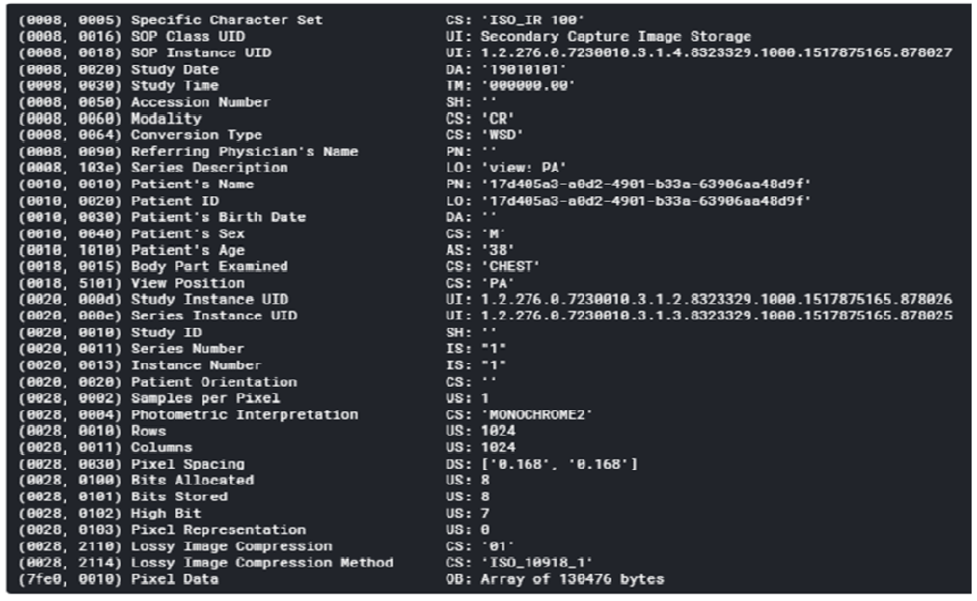
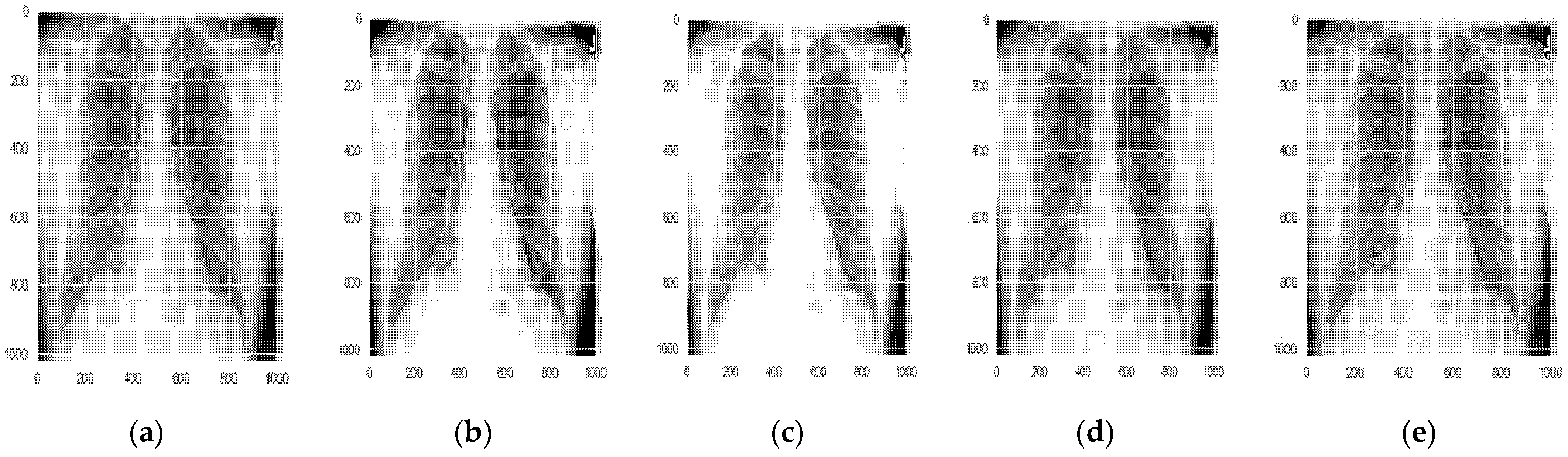
3. Dataset Analysis
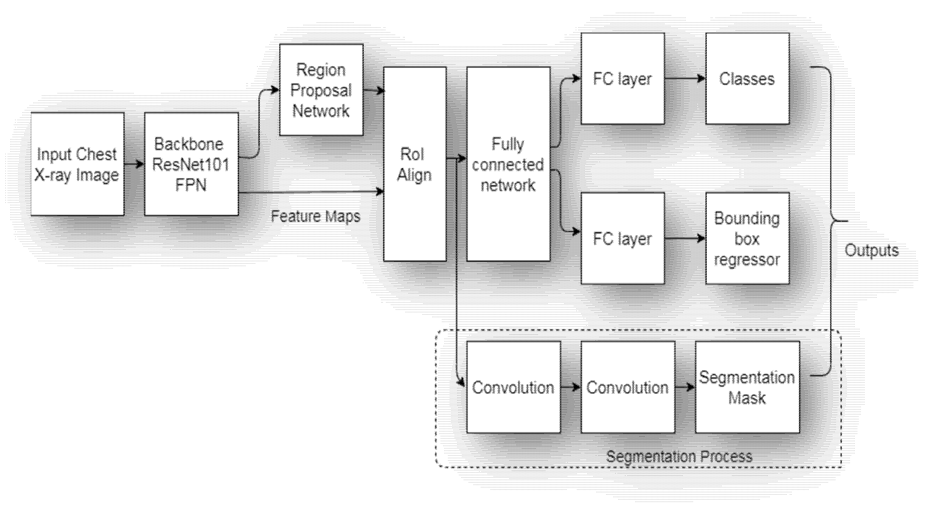
4. Architecture of Proposed Mask RCNN Model
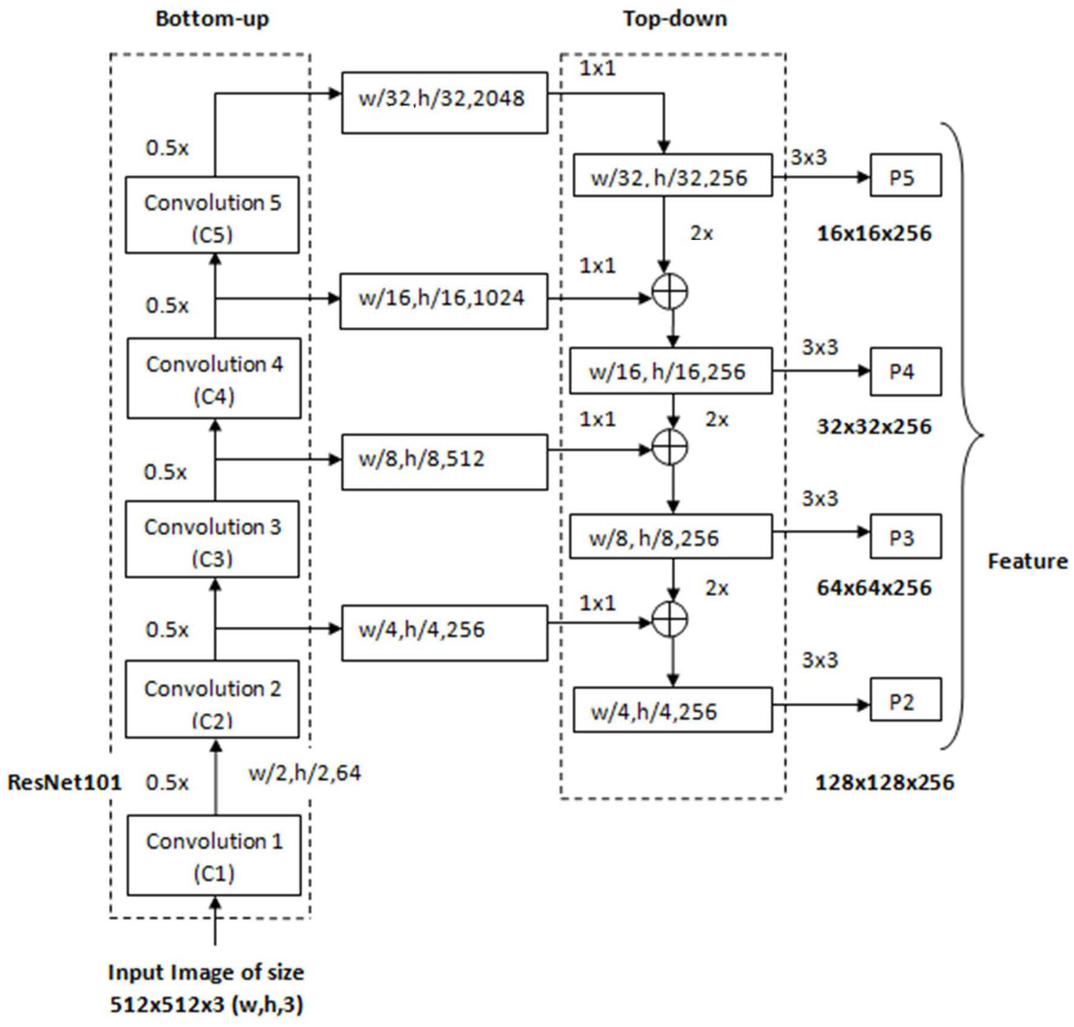
4.1. Backbone ResNet101 Feature Pyramid Network (FPN)
4.2. Regional Proposal Network
- (i)
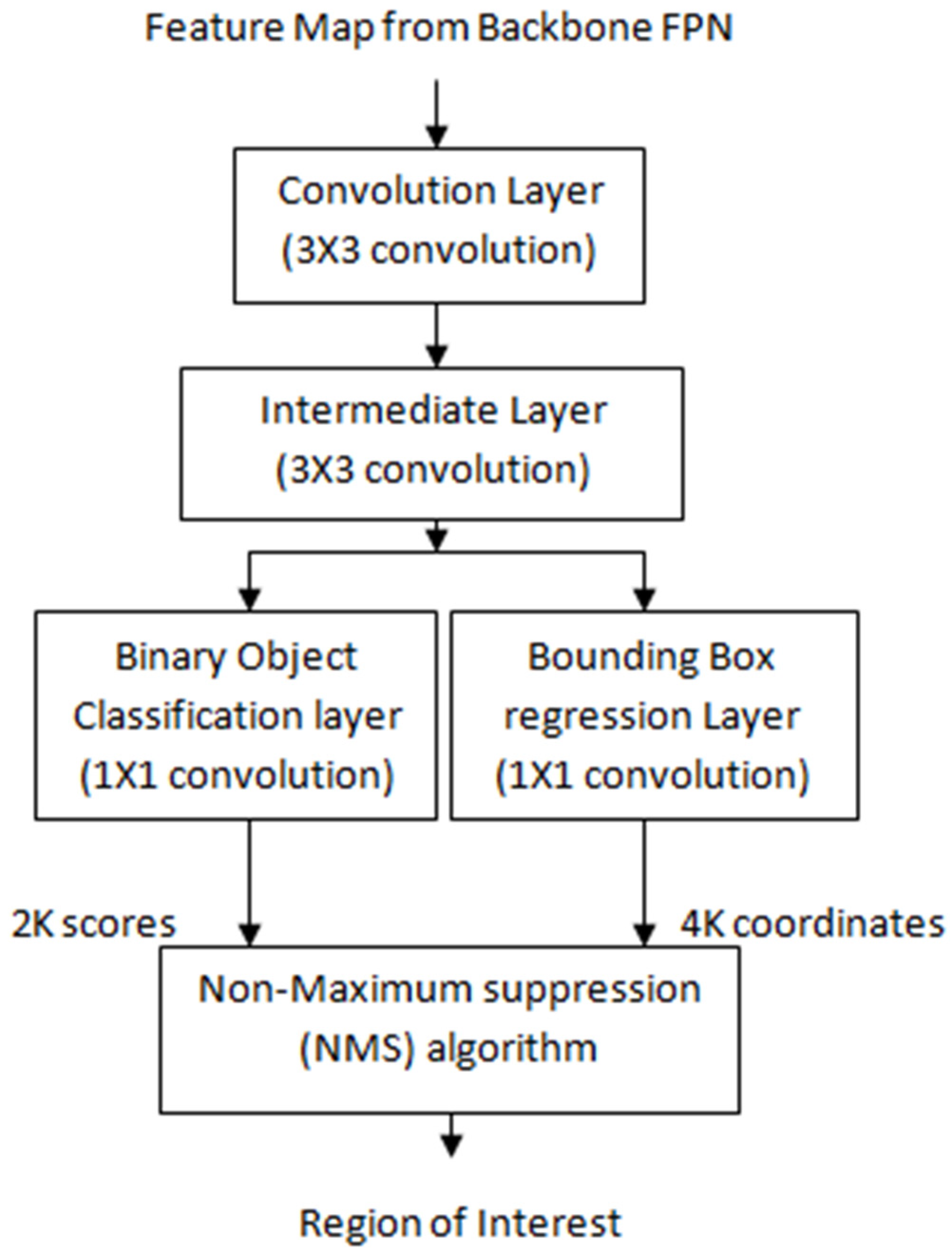
- Anchor generation: A sliding window convolution of 3 × 3 (with 512 filters and padding = same) is applied to the feature maps obtained from the backbone feature pyramid network. The center point of the sliding window represents an anchor. In the proposed model, anchor boxes have a scale of {322, 642, 1282, 2562} pixels with anchor ratios of {1:2, 1:1, 2:1}. Each sliding window of RPN generates K = 12 anchor boxes with four scales and three aspect ratios. For the entire image, N = W × H × K anchor boxes are generated with W*H being the size of input convolution feature maps. Figure 5 shows the process of the anchor generation.
- (ii)
- Classification scores and bounding box coordinates generation: The anchor or bounding boxes generated in the previous step are passed to an intermediate layer of 3 × 3 convolution (with padding of one) and 256 output channels. As depicted in Figure 6, the output is then passed to two layers of 1 × 1 convolution: the classification layer and regression layer. The classification layer generates a matrix of size (W, H, k × 2) for N anchor boxes with two scores corresponding to the probability of an object existing or not. The regression layer generates a matrix of size (W, H, k × 4) for N anchor boxes with four values of the coordinates of each bounding box (see Figure 5).
- (iii)
- Non maximum suppression (NMS) algorithm: Out of the generated bounding boxes, the best bounding boxes were selected using the non maximum suppression (NMS) algorithm given below:
- (a)
- Sort all of the created bounding boxes in decreasing order of their object score confidence;
- (b)
- Select the box with the highest object score confidence;
- (c)
- Calculate the overlap or intersection over union (IoU) of the current box with the other boxes that belong to the same object class;
- (d)
- Remove all the boxes with IoU values greater than 0.7;
- (e)
- Move to the next highest object score confidence;
- (f)
- Repeat the above steps for all the boxes in the list.
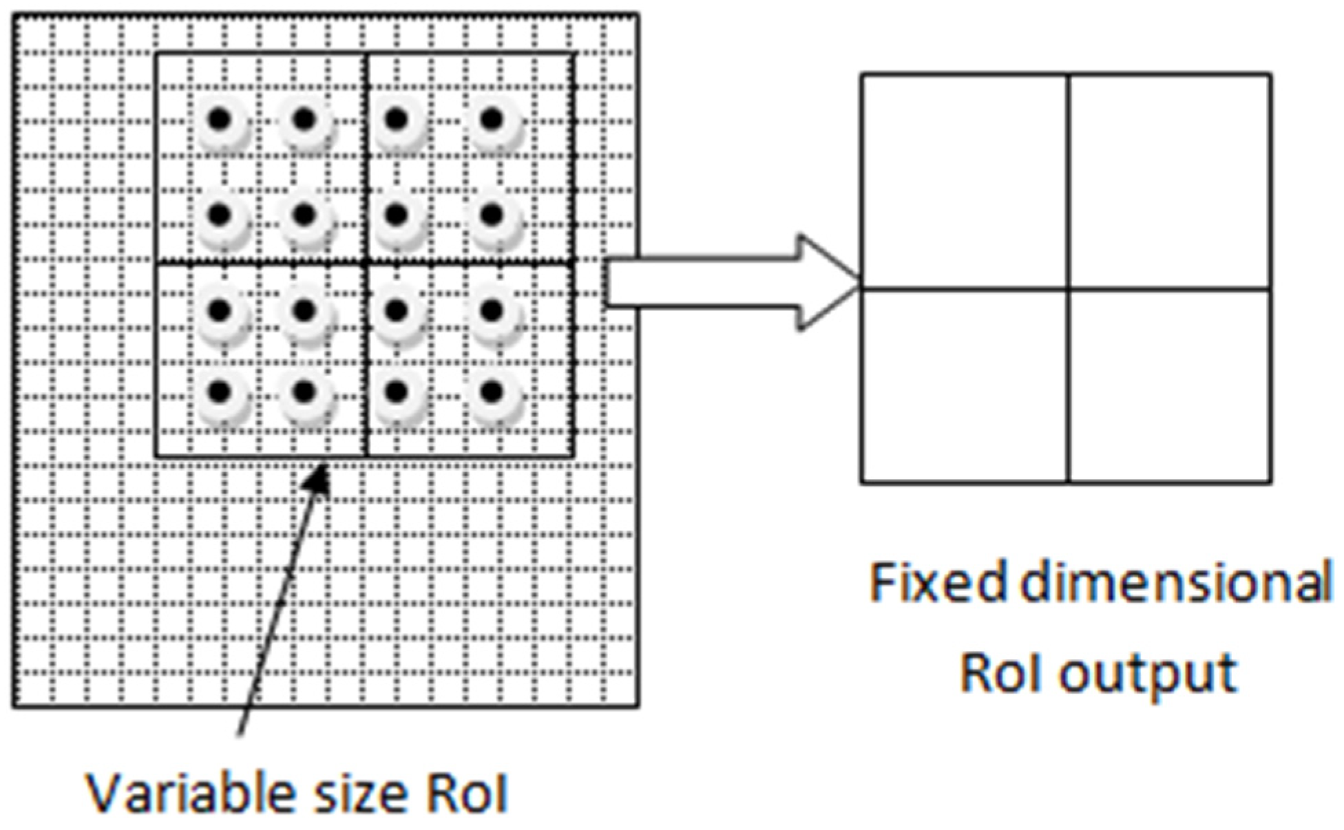
4.3. Region of Interest (RoI) Align
- (a)
- The region proposal candidates are generated by RPN. These region proposal coordinates are floating point numbers, and their boundaries are not quantized.
- (b)
- The region proposal candidate boxes are divided evenly into a fixed number of smaller regions.
- (c)
- In each smaller region, four points are sampled.
- (d)
- The feature pixel values for each point are calculated using bilinear interpolation.
- (e)
- The max-pooling operation is performed on each subregion to obtain the final feature map.
4.4. Segmentation Process
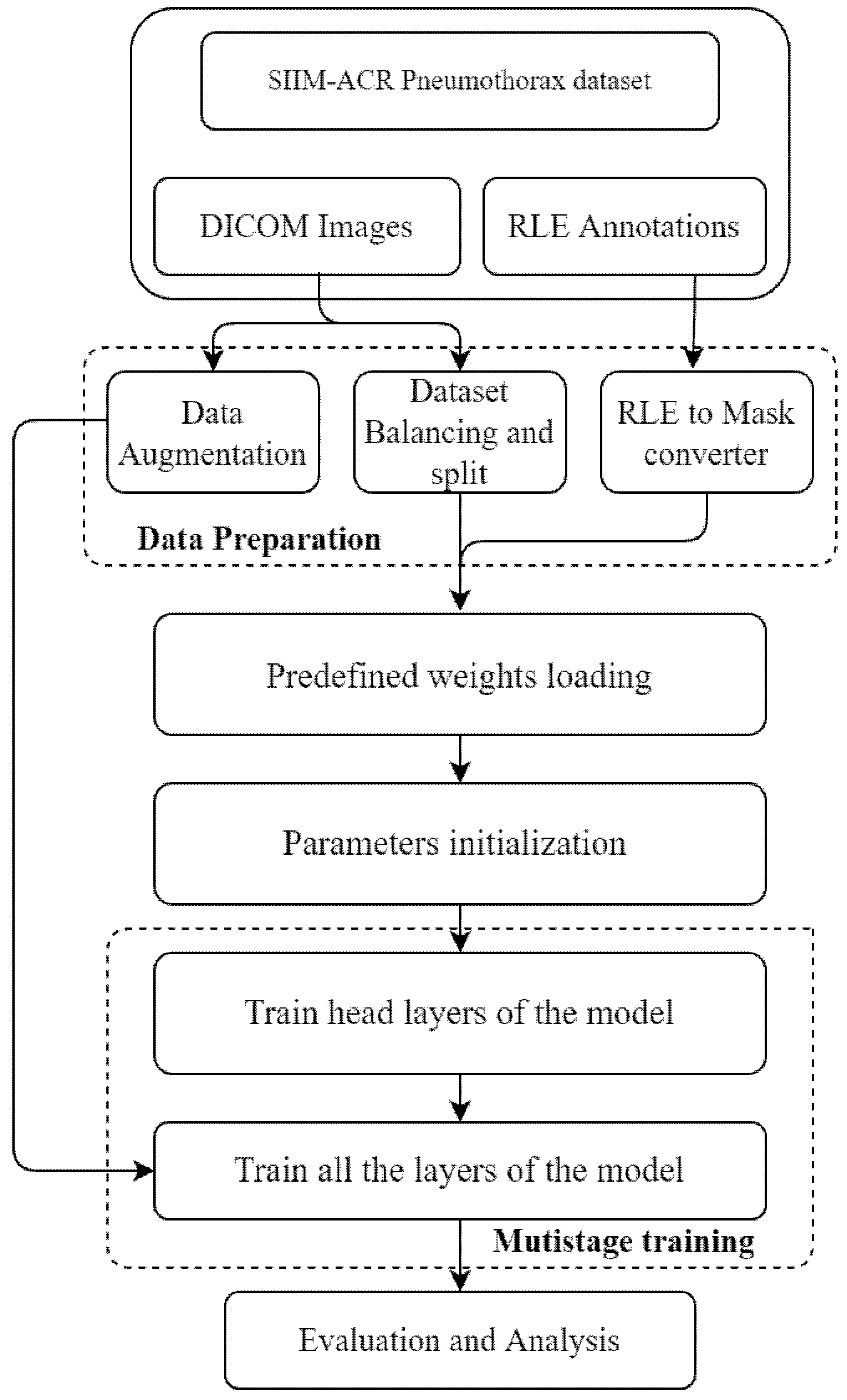
5. Workflow of Proposed Model
5.1. Data Preparation
5.1.1. Data Augmentation
5.1.2. Dataset Balancing and Splitting
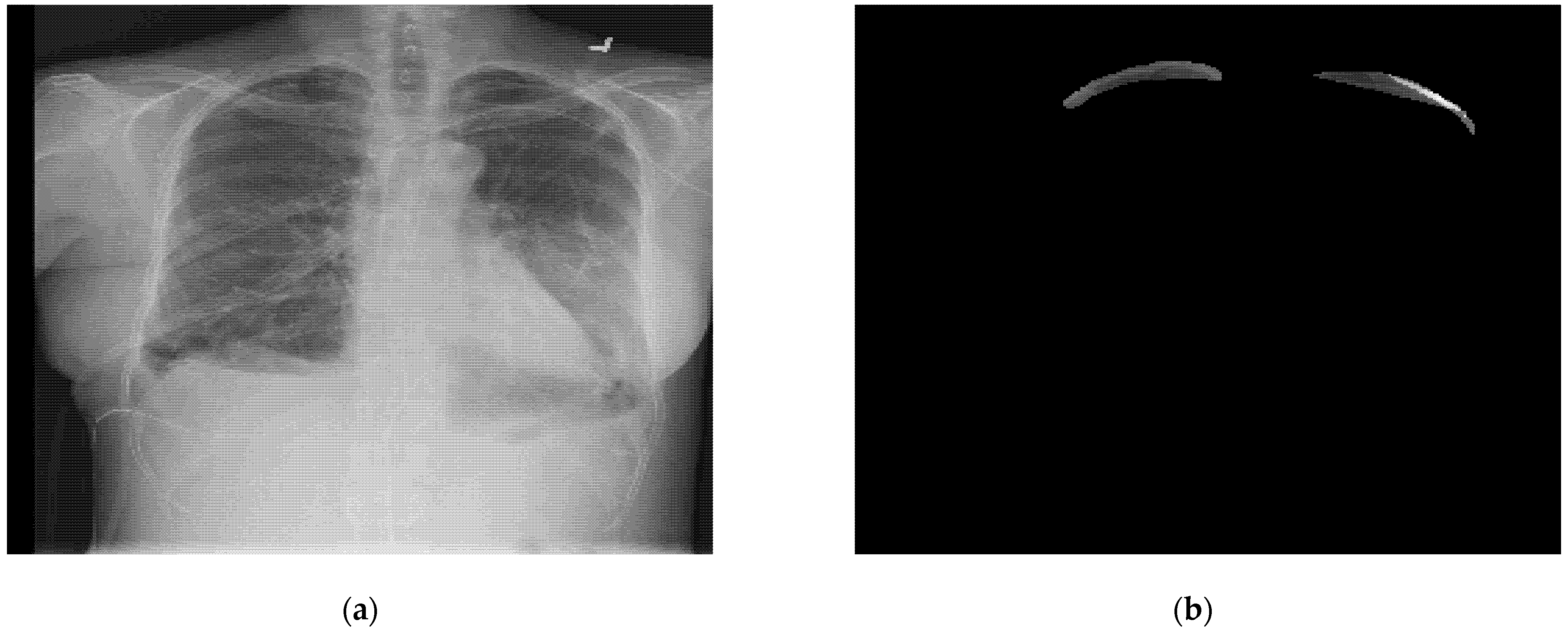
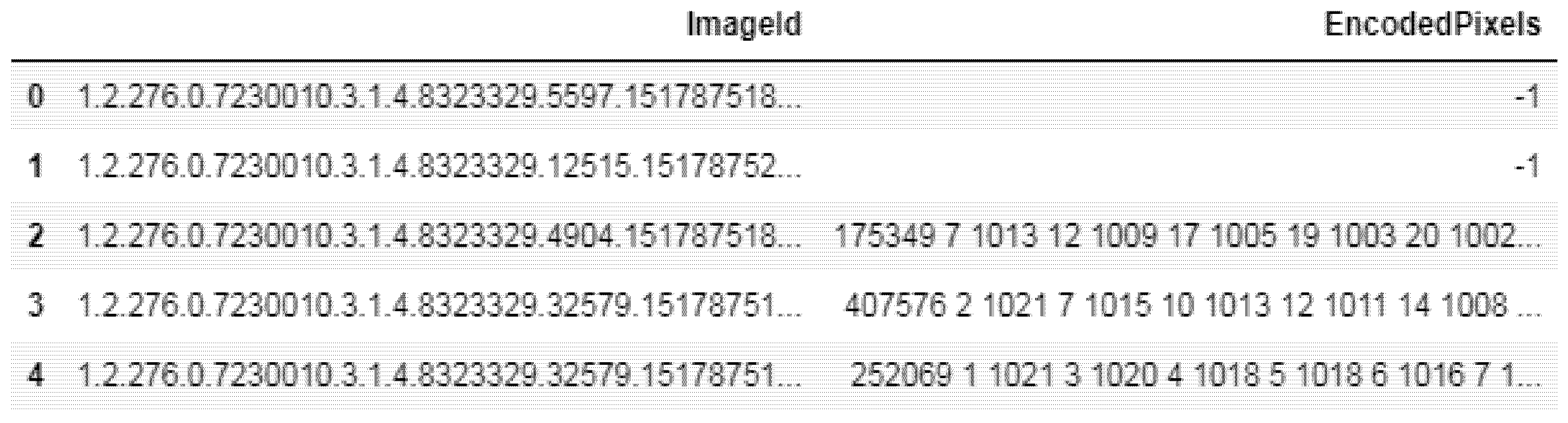
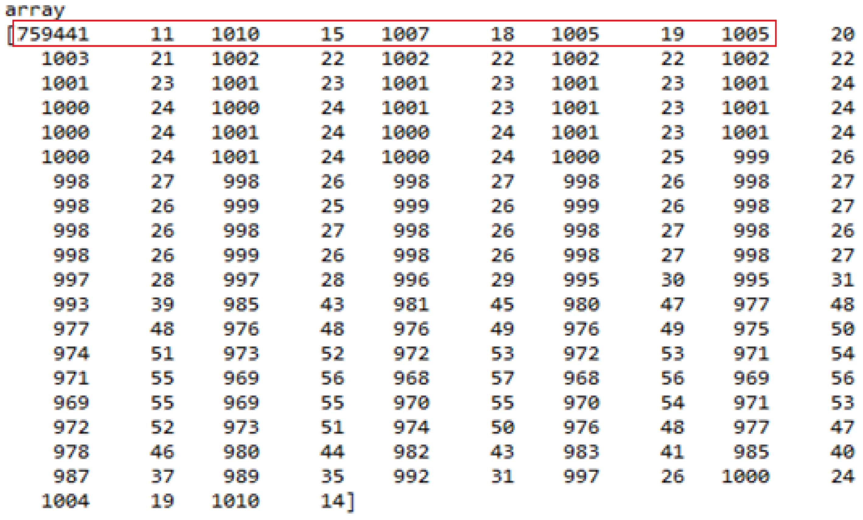
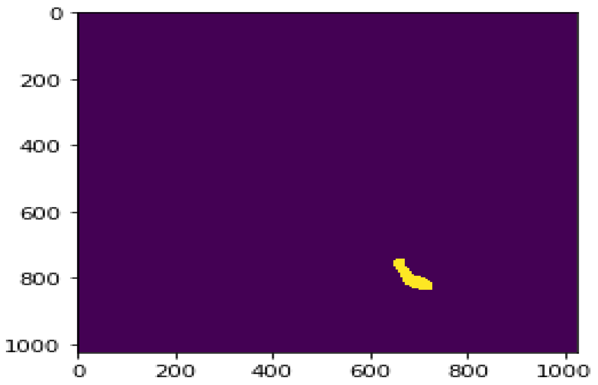
5.1.3. RLE to Mask Conversion
5.2. Predefined Weights Loading
5.3. Parameter Initialization
5.4. Multistage Training
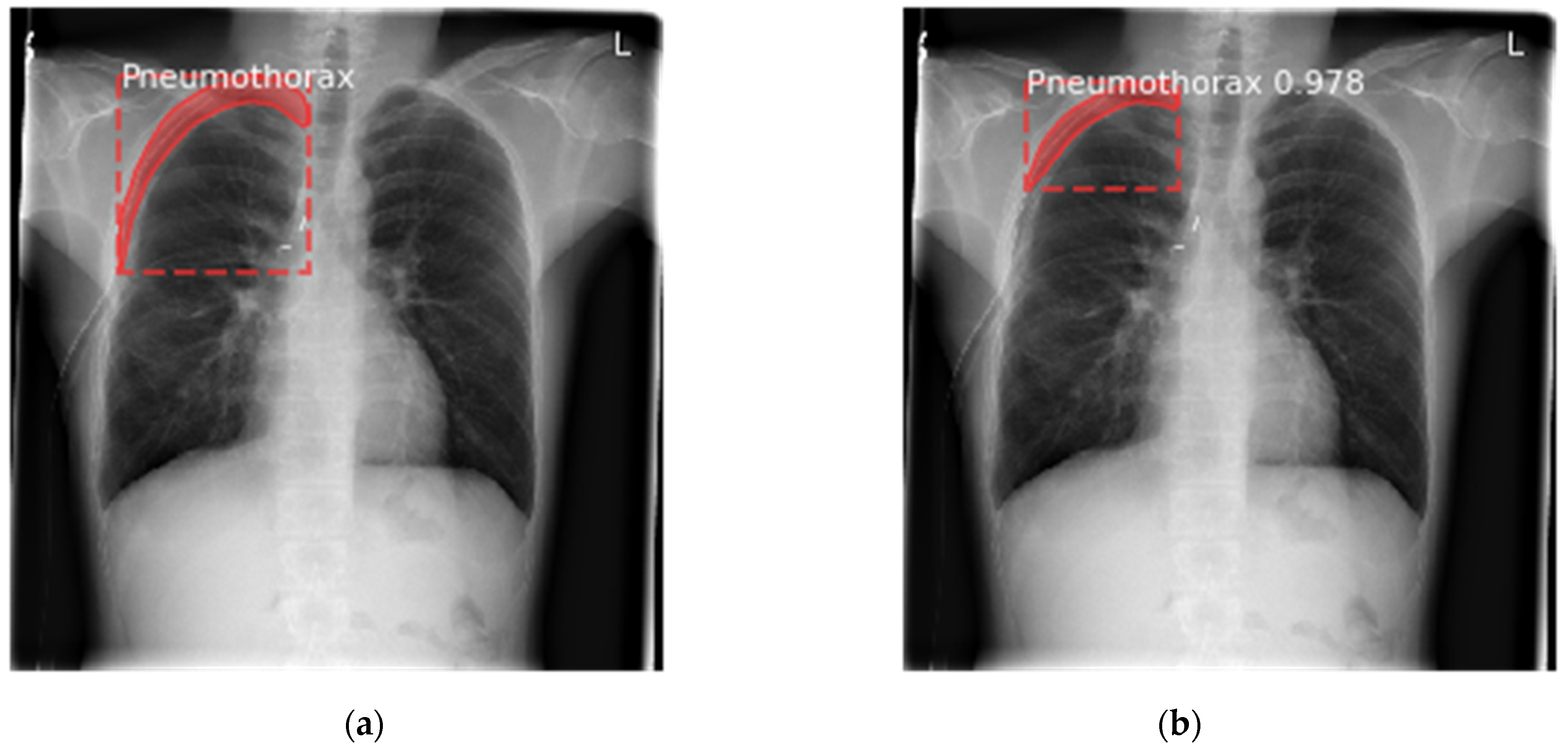
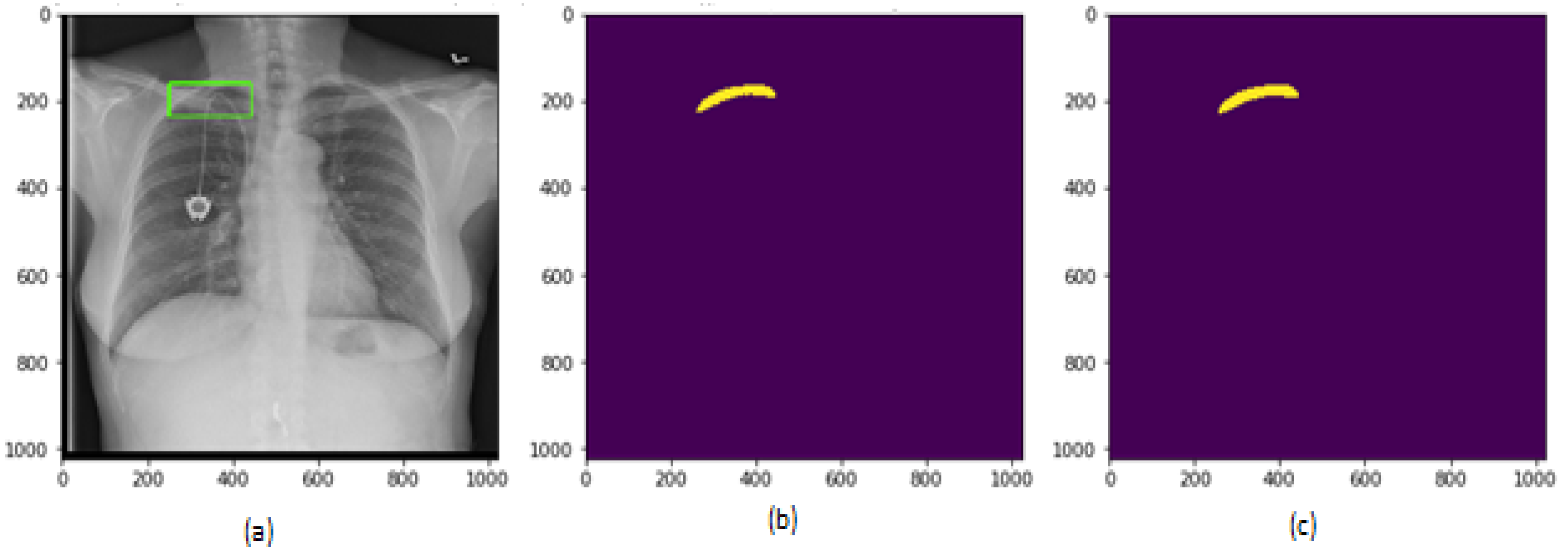
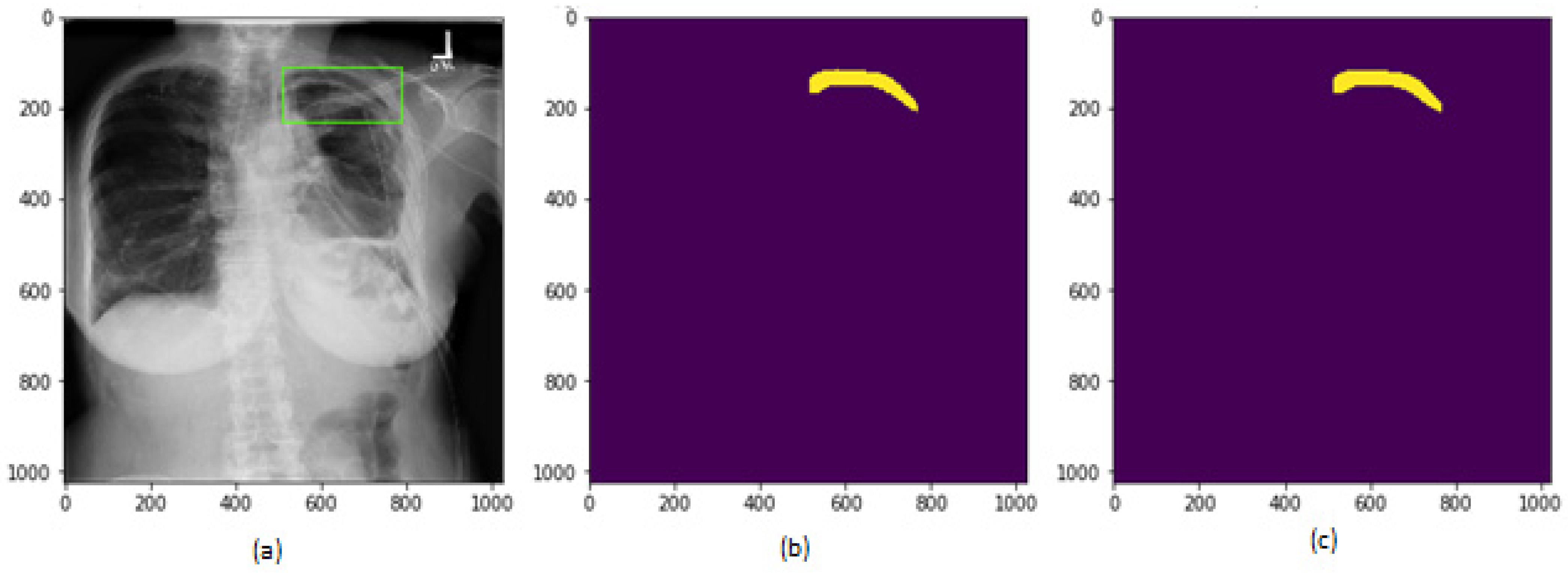
6. Results and Discussion
6.1. Results for Segmentation of Pneumothorax
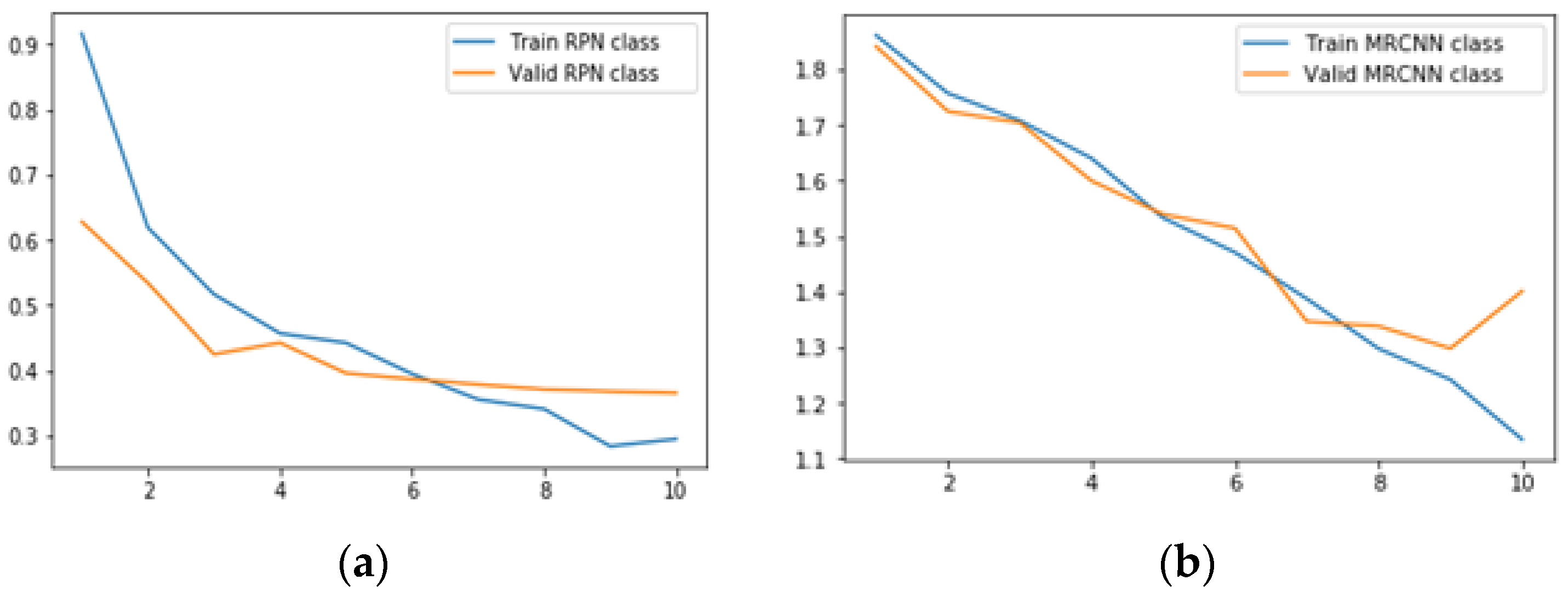
6.2. Analysis Based on Loss Scores
6.2.1. Results for Class Loss
- (a)
- RPN class loss is defined as the RPN anchor classifier loss that represents the closeness of the RPN in predicting the class label.
- (b)
- MRCNN class loss represents the loss due to the classifier head of the Mask RCNN.
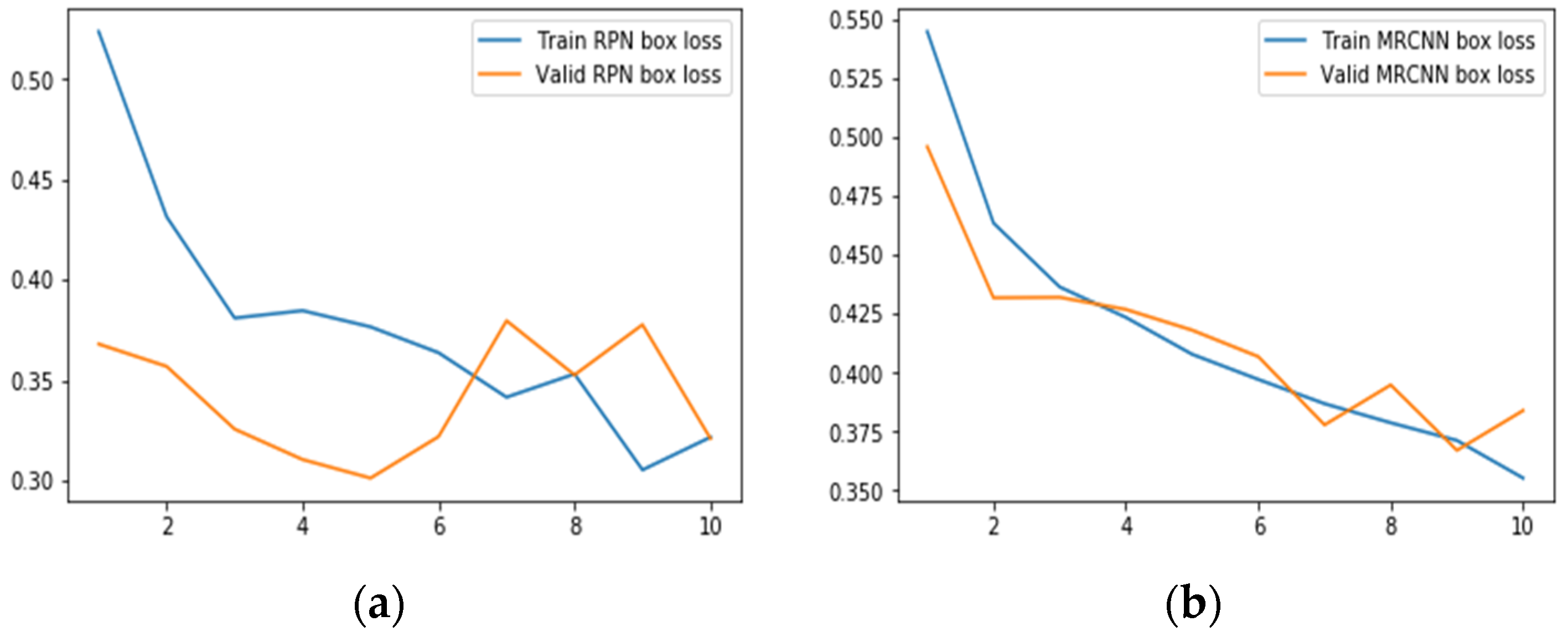
6.2.2. Results for Bounding Box Regression Loss
- (a)
- RPN bbox loss provides the RPN bounding box loss values reflecting the distance between the true boxes coordinates and the predicted RPN boxes coordinates.
- (b)
- MRCNN bbox loss provides the MRCNN bounding box loss values reflecting the distance between the true boxes coordinates and the predicted MRCNN coordinates. Smooth L1 loss [37,38] is used to represent bounding box regression as shown in Equations (3) and (4).Here, λ represents the balancing parameter set to 10.Nbox is the normalization term equal to the number of anchor locations, set to 256.Pi represents the predicted probability that anchor i is an object.Pi* L1 shows that regression loss is active for positive anchors (Pi* = 1) only.ti represents the predicted four coordinates.ti* represents ground truth coordinates.
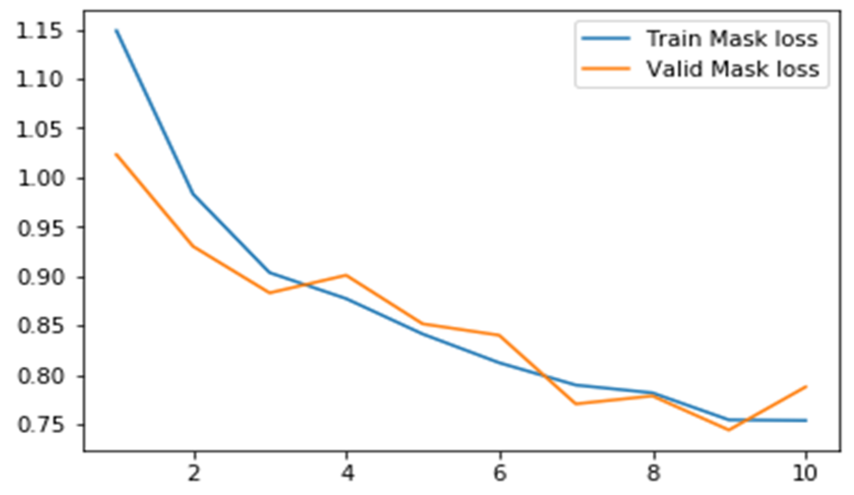
6.2.3. Results for Mask Loss
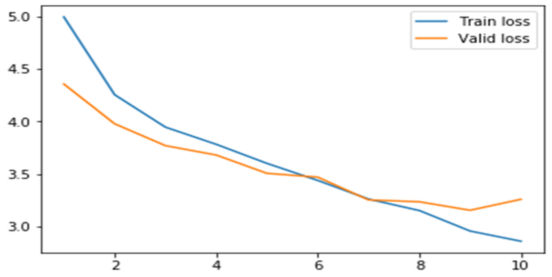
6.2.4. Results for Total Loss
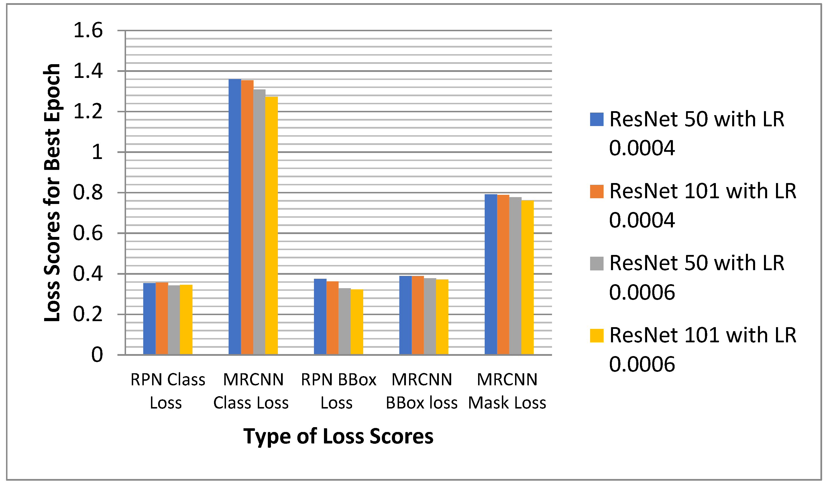
6.2.5. Analysis of the Proposed Model for All the Losses
6.3. Comparison with Existing Models
7. Conclusions and Future Scope
Author Contributions
Funding
Institutional Review Board Statement
Informed Consent Statement
Data Availability Statement
Acknowledgments
Conflicts of Interest
References
- Sahn, S.A.; Heffner, J.E. Spontaneous pneumothorax. N. Engl. J. Med. 2000, 342, 868–874. [Google Scholar] [CrossRef] [PubMed]
- Williams, K.; Oyetunji, T.A.; Hsuing, G.; Hendrickson, R.J.; Lautz, T.B. Spontaneous Pneumothorax in Children: National Management Strategies and Outcomes. J. Laparoendosc. Adv. Surg. Tech. A 2018, 28, 218–222. [Google Scholar] [CrossRef] [PubMed]
- Rami, K.; Damor, P.; Upadhyay, G.; Thakor, N. Profile of patients of spontaneous pneumothorax of North Gujarat region, India: A prospective study at GMERS medical college, Dharpur-Patan. Int. J. Res. Med. Sci. 2015, 3, 1874–1877. [Google Scholar] [CrossRef][Green Version]
- Wakai, A.P. Spontaneous pneumothorax. BMJ Clin. Evid. 2011, 2011, 1505. [Google Scholar]
- Martinelli, A.W.; Ingle, T.; Newman, J.; Nadeem, I.; Jackson, K.; Lane, N.D.; Melhorn, J.; Davies, H.E.; Rostron, A.J.; Adeni, A.; et al. COVID-19 and pneumothorax: A multicentre retrospective case series. Eur. Respir. J. 2020, 56, 2002697. [Google Scholar] [CrossRef]
- Doi, K.; MacMahon, H.; Katsuragawa, S.; Nishikawa, R.; Jiang, Y. Computer-aided diagnosis in radiology: Potential and pitfalls. Eur. J. Radiol. 1999, 31, 97–109. [Google Scholar] [CrossRef]
- Verma, D.R. Managing DICOM Images: Tips and tricks for the radiology and imaging. J. Digit. Imaging 2012, 22, 4–13. [Google Scholar]
- Rimmer, A. Radiologist shortage leaves patient care at risk, warns royal college. BMJ 2017, 359, j4683. [Google Scholar] [CrossRef]
- Malhotra, P.; Gupta, S.; Koundal, D. Computer Aided Diagnosis of Pneumonia from Chest Radiographs. J. Comput. Theor. Nanosci. 2019, 16, 4202–4213. [Google Scholar] [CrossRef]
- Sharma, N.; Aggarwal, L.M. Automated medical image segmentation techniques. J. Med. Phys. 2010, 35, 3. [Google Scholar] [CrossRef]
- Yuheng, S.; Hao, Y. Image segmentation algorithms overview. arXiv 2017, arXiv:1707.02051. [Google Scholar]
- SIIM ACR Pneumothorax Segmentation Data. Available online: https://www.kaggle.com (accessed on 19 July 2021).
- Girshick, R.; Donahue, J.; Darrell, T.; Malik, J. Rich feature hierarchies for accurate object detection and semantic segmentation. In Proceedings of the IEEE Conference on Computer Vision and Pattern Recognition, Columbus, OH, USA, 23–28 June 2014; pp. 580–587. [Google Scholar]
- Baumgartner, C.F.; Koch, L.M.; Pollefeys, M.; Konukoglu, E. An Exploration of 2D and 3D Deep Learning Techniques for Cardiac MR Image Segmentation. In Statistical Atlases and Computational Models of the Heart. ACDC and MMWHS Challenges; STACOM 2017; Pop, M., Ed.; Springer: Cham, Switzerland, 2018; pp. 111–119. [Google Scholar] [CrossRef]
- Cai, J.; Lu, L.; Xing, F.; Yang, L. Pancreas segmentation in CT and MRI images via domain specific network designing and recurrent neural contextual learning. arXiv 2018, arXiv:1803.11303. [Google Scholar]
- Chen, H.; Dou, Q.; Yu, L.; Qin, J.; Heng, P.-A. VoxResNet: Deep voxelwise residual networks for brain segmentation from 3D MR images. NeuroImage 2018, 170, 446–455. [Google Scholar] [CrossRef] [PubMed]
- Christ, P.F.; Ettlinger, F.; Grün, F.; Elshaera, M.E.A.; Lipkova, J.; Schlecht, S.; Ahmaddy, F.; Tatavarty, S.; Bickel, M.; Bilic, P.; et al. Automatic liver and tumor segmentation of CT and MRI volumes using cascaded fully convolutional neural networks. arXiv 2017, arXiv:1702.05970. [Google Scholar]
- Dou, Q.; Chen, H.; Jin, Y.; Yu, L.; Qin, J.; Heng, P.A. 3D deeply supervised network for automatic liver segmentation from CT volumes. In Proceedings of the International Conference on Medical Image Computing and Computer-Assisted Intervention, Athens, Greece, 17–21 October 2016; Springer: Cham, Switzerland, 2016; pp. 149–157. [Google Scholar]
- Dhungel, N.; Carneiro, G.; Bradley, A.P. Deep learning and structured prediction for the segmentation of mass in mammograms. In Eighteenth International Conference on Medical Image Computing and Computer-Assisted Intervention, Munich, Germany, 5–9 October 2015; Springer: Cham, Switzerland, 2015; pp. 605–612. [Google Scholar]
- Poudel, R.P.K.; Lamata, P.; Montana, G. Recurrent Fully Convolutional Neural Networks for Multi-slice MRI Cardiac Segmentation. In Reconstruction, Segmentation, and Analysis of Medical Images; RAMBO 2016, HVSMR 2016; Zuluaga, M., Bhatia, K., Kainz, B., Moghari, M., Pace, D., Eds.; Springer: Cham, Switzerland, 2017; pp. 83–94. [Google Scholar] [CrossRef]
- Hamidian, S.; Sahiner, B.; Petrick, N.; Pezeshk, A. 3D convolutional neural network for automatic detection of lung nodules in Chest CT. In Medical Imaging 2017: Computer-Aided Diagnosis; International Society for Optics and Photonics: Bellingham, WA, USA, 2017; Volume 10134, p. 1013409. [Google Scholar]
- Stollenga, M.F.; Byeon, W.; Liwicki, M.; Schmidhuber, J. Parallel multi-dimensional lstm, with application to fast biomedical volumetric image segmentation. In Advances in Neural Information Processing System, Proceedings of the Annual Conference on Neural Information Processing Systems, Montreal, QC, Canada, 7–12 December 2015; Curran Associates, Inc.: Red Hook, NY, USA, 2015; pp. 2998–3006. [Google Scholar]
- Zhang, J.; Lv, X.; Sun, Q.; Zhang, Q.; Wei, X.; Liu, B. SDResU-Net: Separable and Dilated Residual U-Net for MRI Brain Tumor Segmentation. Curr. Med. Imaging 2020, 16, 720–728. [Google Scholar] [CrossRef] [PubMed]
- Milletari, F.; Navab, N.; Ahmadi, S.-A. V-Net: Fully convolutional neural networks for volumetric medical image segmentation. In Proceedings of the Fourth International Conference on 3D Vision (3DV), Stanford, CA, USA, 25–28 October 2016; pp. 565–571. [Google Scholar]
- Mulay, S.; Deepika, G.; Jeevakala, S.; Ram, K.; Sivaprakasam, M. Liver Segmentation from Multimodal Images Using HED-Mask R-CNN. In Proceedings of the International Workshop on Multiscale Multimodal Medical Imaging, Shenzhen, China, 13 October 2019; Springer: Cham, Switzerland, 2019; pp. 68–75. [Google Scholar]
- Gordienko, Y.; Gang, P.; Hui, J.; Zeng, W.; Kochura, Y.; Alienin, O.; Rokovyi, O.; Stirenko, S. Deep learning with lung segmentation and bone shadow exclusion techniques for chest X-ray analysis of lung cancer. In Proceedings of the Fifth International Conference on Computer Science, Engineering and Education Applications, Kyiv, Ukraine, 21–22 February 2022; Springer: Cham, Switzerland, 2018; pp. 638–647. [Google Scholar]
- Gooßen, A.; Deshpande, H.; Harder, T.; Schwab, E.; Baltruschat, I.; Mabotuwana, T.; Cross, N.; Saalbach, A. Pneumothorax detection and localization in chest radiographs: A comparison of deep learning approaches. In Proceedings of the Second International Conference on Medical Imaging with Deep Learning (MIDL 2019), London, UK, 8–10 July 2019. [Google Scholar]
- Taylor, A.G.; Mielke, C.; Mongan, J. Automated detection of moderate and large pneumothorax on frontal chest X-rays using deep convolutional neural networks: A retrospective study. PLoS Med. 2018, 15, e1002697. [Google Scholar] [CrossRef] [PubMed]
- Wang, H.; Gu, H.; Qin, P.; Wang, J. CheXLocNet: Automatic localization of pneumothorax in chest radiographs using deep convolutional neural networks. PLoS ONE 2020, 15, e0242013. [Google Scholar] [CrossRef]
- Abedalla, A.; Abdullah, M.; Al-Ayyoub, M.; Benkhelifa, E. The 2ST-UNet for Pneumothorax Seg-mentation in Chest X-rays using ResNet34 as a Backbone for U-Net. arXiv 2020, arXiv:2009.02805. [Google Scholar]
- Groza, V.; Kuzin, A. Pneumothorax Segmentation with Effective Conditioned Post-Processing in Chest X-ray. In Proceedings of the 17th International Symposium on Biomedical Imaging Workshops (ISBI Workshops), Iowa City, IA, USA, 4 April 2020; pp. 1–4. [Google Scholar]
- He, K.; Gkioxari, G.; Dollár, P.; Girshick, R. Mask R-CNN. In Proceedings of the IEEE International Conference on Computer Vision (ICCV), Venice, Italy, 22–29 October 2017; pp. 2961–2969. [Google Scholar]
- He, K.; Zhang, X.; Ren, S.; Sun, J. Deep Residual Learning for Image Recognition. In Proceedings of the IEEE Conference on Computer Vision and Pattern Recognition, Las Vegas, NV, USA, 27–30 June 2016; pp. 770–778. [Google Scholar]
- Gonzalez, S.; Arellano, C.; Tapia, J.E. Deepblueberry: Quantification of Blueberries in the Wild Using Instance Segmentation. IEEE Access 2019, 7, 105776–105788. [Google Scholar] [CrossRef]
- Lin, T.Y.; Dollár, P.; Girshick, R.; He, K.; Hariharan, B.; Belongie, S. Feature pyramid networks for object detection. In Proceedings of the IEEE Conference on Computer Vision and Pattern Recognition, Honolulu, HI, USA, 21–26 July 2017; pp. 2117–2125. [Google Scholar]
- Weiss, K.; Khoshgoftaar, T.M.; Wang, D.D. A survey of transfer learning. J. Big Data 2016, 3, 1345–1459. [Google Scholar] [CrossRef]
- Ren, S.; He, K.; Girshick, R.; Sun, J. Faster R-CNN: Towards real-time object detection with region proposal networks. IEEE Trans. Pattern Anal. Mach. Intell. 2016, 39, 1137–1149. [Google Scholar] [CrossRef] [PubMed]
- Ahmed, I.; Ahmad, M.; Rodrigues, J.J.; Jeon, G.; Din, S. A deep learning-based social distance monitoring framework for COVID-19. Sustain. Cities Soc. 2020, 65, 102571. [Google Scholar] [CrossRef] [PubMed]
- Ahmed, I.; Ahmad, M.; Jeon, G. Social distance monitoring framework using deep learning architecture to control infection transmission of COVID-19 pandemic. Sustain. Cities Soc. 2021, 69, 102777. [Google Scholar] [CrossRef]
- Girshick, R. Fast R-CNN. In Proceedings of the IEEE International Conference on Computer Vision, Santiago, Chile, 7–13 December 2014; pp. 1440–1448. [Google Scholar]
- MacDonald, M.; Fennel, T.R.; Singanamalli, A.; Cruz, N.M.; Yousefhussein, M.; Al-Kofahi, Y.; Freedman, B.S. Improved automated segmentation of human kidney organoids using deep convolutional neural networks. In Medical Imaging 2020: Image Processing; International Society for Optics and Photonics: Bellingham, WA, USA, 2020; Volume 11313, p. 113133B. [Google Scholar]
- Perez, L.; Wang, J. The effectiveness of data augmentation in image classification using deep learning. arXiv 2017, arXiv:1712.04621. [Google Scholar]
- Matterport’s Implementation of Mask RCNN. Available online: https://github.com (accessed on 19 July 2021).
- Buragohain, A.; Mali, B.; Saha, S.; Singh, P.K. A deep transfer learning based approach to detect COVID -19 waste. Internet Technol. Lett. 2021, e327. [Google Scholar] [CrossRef]
- Jadon, S. A survey of loss functions for semantic segmentation. In Proceedings of the IEEE Conference on Computational Intelligence in Bioinformatics and Computational Biology (CIBCB), Viña del Mar, Chile, 27–20 October 2020; pp. 1–7. [Google Scholar]
- Zhang, Z.; Sabuncu, M. Generalized cross entropy loss for training deep neural networks with noisy labels. In Advances in Neural Information Processing Systems, 31; MIT Press: Monteal, QC, Canada, 2018. [Google Scholar]
- Zhang, Y.; Chu, J.; Leng, L.; Miao, J. Mask-Refined R-CNN: A Network for Refining Object Details in Instance Segmentation. Sensors 2020, 20, 1010. [Google Scholar] [CrossRef]
- Jakhar, K.; Kaur, A.; Gupta, D. Pneumothorax segmentation: Deep learning image segmentation to predict pneumothorax. arXiv 2019, arXiv:1912.07329. [Google Scholar]
- Kaur, M.; Kumar, V.; Yadav, V.; Singh, D.; Kumar, N.; Das, N.N. Metaheuristic-based Deep COVID-19 Screening Model from Chest X-ray Images. J. Healtc. Eng. 2021, 2021, 8829829. [Google Scholar] [CrossRef]
- Singh, D.; Kumar, V. Single image defogging by gain gradient image filter. Sci. China Inf. Sci. 2019, 62, 79101. [Google Scholar] [CrossRef]
- Singh, D.; Kumar, V. Dehazing of outdoor images using notch based integral guided filter. Multimed. Tools Appl. 2018, 77, 27363–27386. [Google Scholar] [CrossRef]


| Layer Name | ResNet50 | Resnet101 |
|---|---|---|
| Convolution 1 | 7 × 7, 64, stride 2 | |
| Convolution 2× | 3 × 3 Max pool, stride 2 | |
| Convolution 3× | ||
| Convolution 4× | ||
| Convolution 5× | ||
| Average pool, 1000-d FC, softmax | ||
| S. No. | Simulation Parameter | Parameter Value |
|---|---|---|
| 1 | RPN anchors per image | 256 |
| 2 | Anchor areas | 322, 642, 1282, 2562 |
| 3 | Anchor ratios | 0.5, 1, 2 |
| 4 | Anchor stride | 1 |
| 5 | RPN NMS Threshold | 0.7 |
| Number of | Before Sampling | After Sampling |
|---|---|---|
| Training Images | 10,675 | 15,629 |
| Validation Images | — | 1320 |
| Test Images | 1377 | 1377 |
| Images with Pneumothorax | 2379 | 8316 |
| Percentage of Positive Cases (%) | 22.29 | 53.21 |
| Initial Pixel Position | Length of Pixels Having Value ‘1’ | Final Pixel Position | Length of Pixels Having Value ‘0’ |
|---|---|---|---|
| 759,441 | 11 | 759,452 | 1010 |
| 760,462 | 15 | 760,477 | 1007 |
| 761,484 | 18 | 761,502 | 1005 |
| 762,507 | 19 | 762,526 | 1005 |
| S. No. | Simulation Parameter Name | Parameter Value | S. No. | Simulation Parameter Name | Parameter Value |
|---|---|---|---|---|---|
| 1 | Number of classes | 2 | 7 | GPU count | 1 |
| 2 | Image dimension | 512 × 512 | 8 | Images per GPU | 11 |
| 3 | RPN anchor scales | 32,64,128,256 | 9 | Weight Decay | 0.0005 |
| 4 | Train RoIs per image | 32 | 10 | Learning momentum | 0.9 |
| 5 | NMS threshold | 0.1 | 11 | Steps per epoch | 350 |
| 6 | Batch size | 11 | 12 | Validation Steps | 120 |
| Sr. No. | Simulation Parameters | Parameter Value for Stage 1 | Parameter Value for Stage 2 |
|---|---|---|---|
| 1 | Learning rate | 0.0012 | 0.0006 |
| 0.0008 | 0.0004 | ||
| 2 | Number of epochs | 1 | 10, 12 |
| 3 | Layers trained | heads | all |
| 4 | Augmentation | None | yes |
| Model | Backbone Network | Learning Rate | Total Epochs | Minimum RPN Class Loss | Minimum MRCNN Class Loss | Total Class Loss = RPN Class Loss + MRCNN Class Loss |
|---|---|---|---|---|---|---|
| Conventional Model | ResNet50 | 0.0004 | 12 | 0.353907 | 1.359199 | 1.713106 |
| Proposed Model | ResNet101 | 12 | 0.355985 | 1.353964 | 1.709949 | |
| Conventional Model | ResNet50 | 0.0006 | 10 | 0.343072 | 1.309230 | 1.652302 |
| Proposed Model | Resnet101 | 10 | 0.345099 | 1.273622 | 1.618721 |
| Model | Backbone Network | Learning Rate | Total Epochs | Minimum RPN BBox Loss | Minimum MRCNN BBox Loss | Total Bbox Loss = RPN BBox Loss + MRCNN BBox Loss |
|---|---|---|---|---|---|---|
| Conventional Model | ResNet50 | 0.0004 | 12 | 0.374971 | 0.389217 | 0.764188 |
| Proposed Model | ResNet101 | 12 | 0.362586 | 0.388650 | 0.751236 | |
| Conventional Model | ResNet50 | 0.0006 | 10 | 0.327884 | 0.378461 | 0.706345 |
| Proposed Model | Resnet101 | 10 | 0.323304 | 0.372548 | 0.645852 |
| Model | Backbone Network | Learning Rate | Total Epochs | Minimum MRCNN Mask Loss |
|---|---|---|---|---|
| Conventional Model | ResNet50 | 0.0004 | 12 | 0.791617 |
| Proposed Model | ResNet101 | 12 | 0.788237 | |
| Conventional Model | ResNet50 | 0.0006 | 10 | 0.777462 |
| Proposed Model | Resnet101 | 10 | 0.760439 |
| Model | Backbone Network | Learning Rate | Total Epochs | Minimum Total Loss | Model Training Time |
|---|---|---|---|---|---|
| Conventional Model | ResNet50 | 0.0004 | 12 | 3.268911 | 31,380 s |
| Proposed Model | ResNet101 | 12 | 3.249549 | 30,430 s | |
| Conventional Model | ResNet50 | 0.0006 | 10 | 3.136109 | 28,800 s |
| Proposed Model | Resnet101 | 10 | 3.075138 | 27,640 s |
Publisher’s Note: MDPI stays neutral with regard to jurisdictional claims in published maps and institutional affiliations. |
© 2022 by the authors. Licensee MDPI, Basel, Switzerland. This article is an open access article distributed under the terms and conditions of the Creative Commons Attribution (CC BY) license (https://creativecommons.org/licenses/by/4.0/).
Share and Cite
Malhotra, P.; Gupta, S.; Koundal, D.; Zaguia, A.; Kaur, M.; Lee, H.-N. Deep Learning-Based Computer-Aided Pneumothorax Detection Using Chest X-ray Images. Sensors 2022, 22, 2278. https://doi.org/10.3390/s22062278
Malhotra P, Gupta S, Koundal D, Zaguia A, Kaur M, Lee H-N. Deep Learning-Based Computer-Aided Pneumothorax Detection Using Chest X-ray Images. Sensors. 2022; 22(6):2278. https://doi.org/10.3390/s22062278
Chicago/Turabian StyleMalhotra, Priyanka, Sheifali Gupta, Deepika Koundal, Atef Zaguia, Manjit Kaur, and Heung-No Lee. 2022. "Deep Learning-Based Computer-Aided Pneumothorax Detection Using Chest X-ray Images" Sensors 22, no. 6: 2278. https://doi.org/10.3390/s22062278
APA StyleMalhotra, P., Gupta, S., Koundal, D., Zaguia, A., Kaur, M., & Lee, H.-N. (2022). Deep Learning-Based Computer-Aided Pneumothorax Detection Using Chest X-ray Images. Sensors, 22(6), 2278. https://doi.org/10.3390/s22062278