
An Unsupervised Deep-Transfer-Learning-Based Motor Imagery EEG Classification Scheme for Brain–Computer Interface


Abstract
:1. Introduction
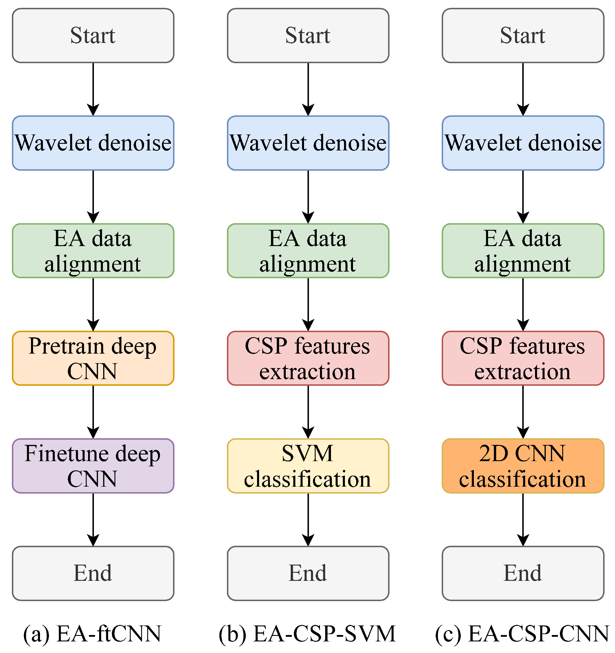
2. Methods
2.1. Wavelet Denoise-Based Preprocessing
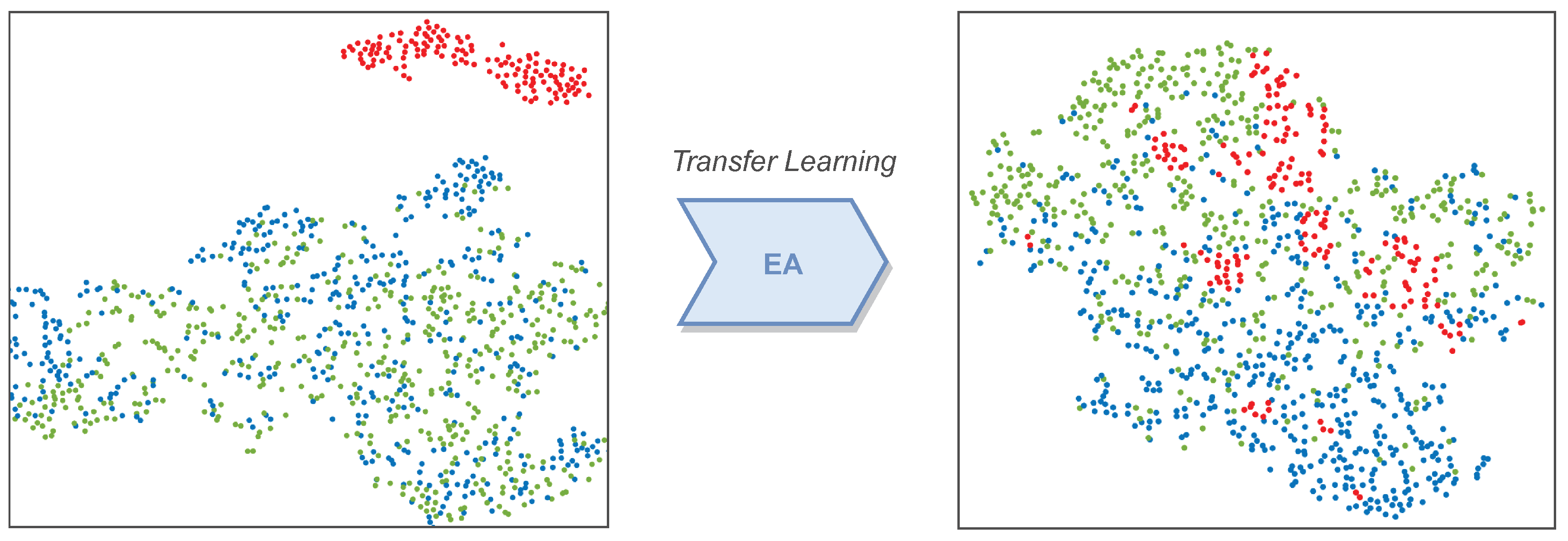
2.2. Euclidean Space Data Alignment Based Preprocessing
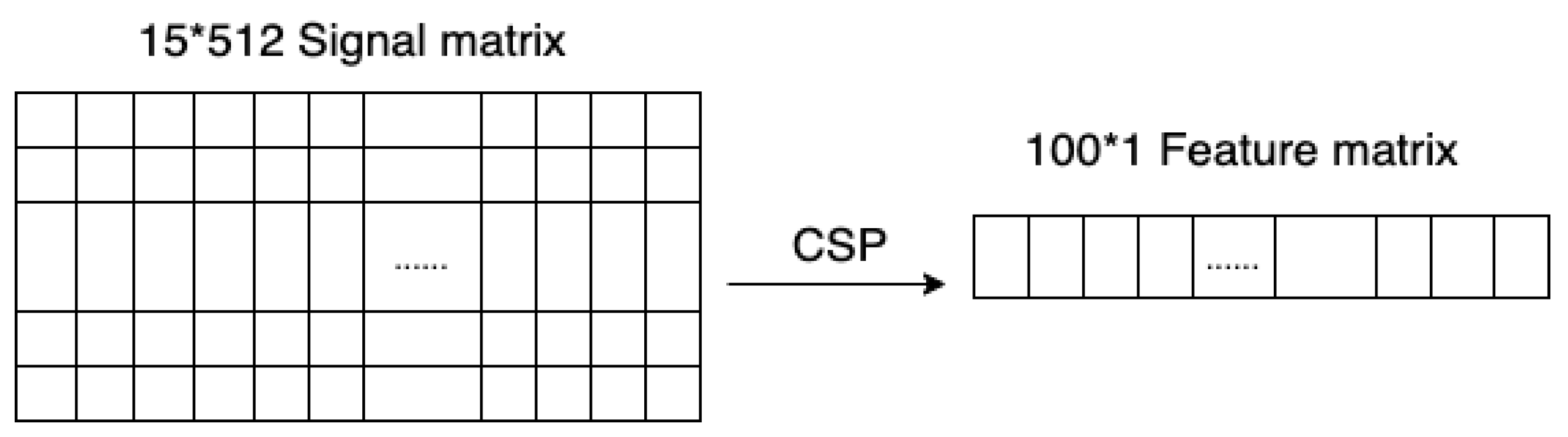
2.3. Common-Spatial-Pattern-Based Feature Extraction
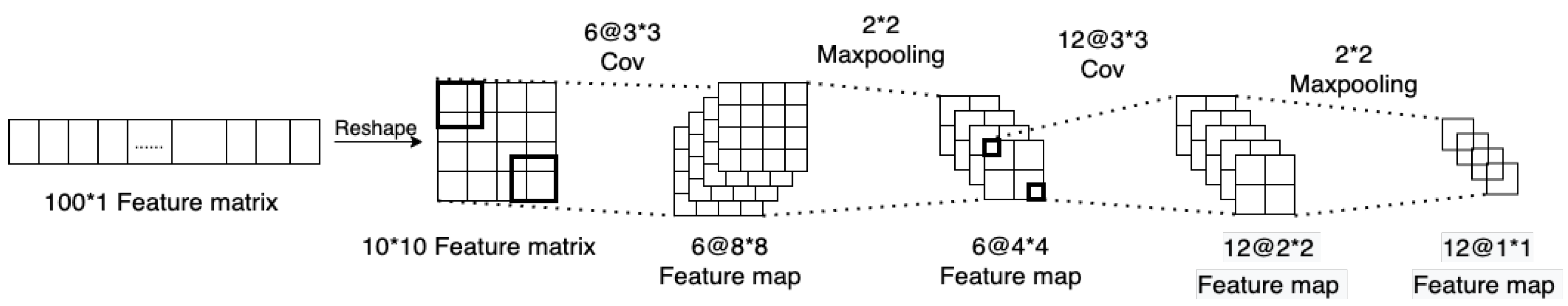
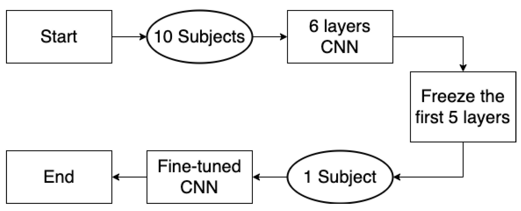
2.4. Convolutional-Neural-Network-Based Classification
3. Experiment and Result Analysis
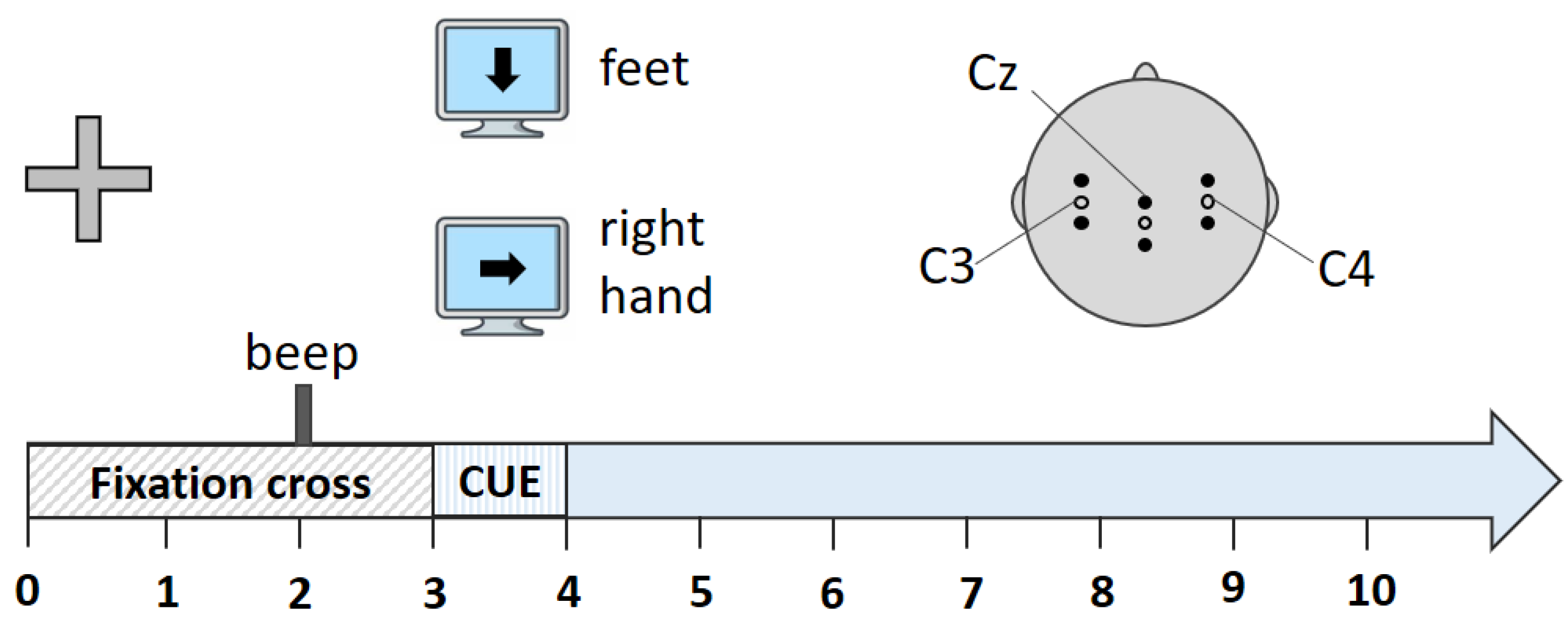
3.1. Dataset Description
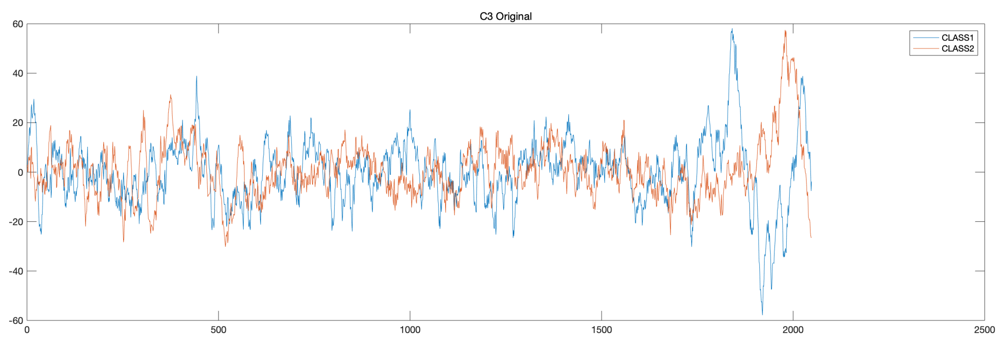
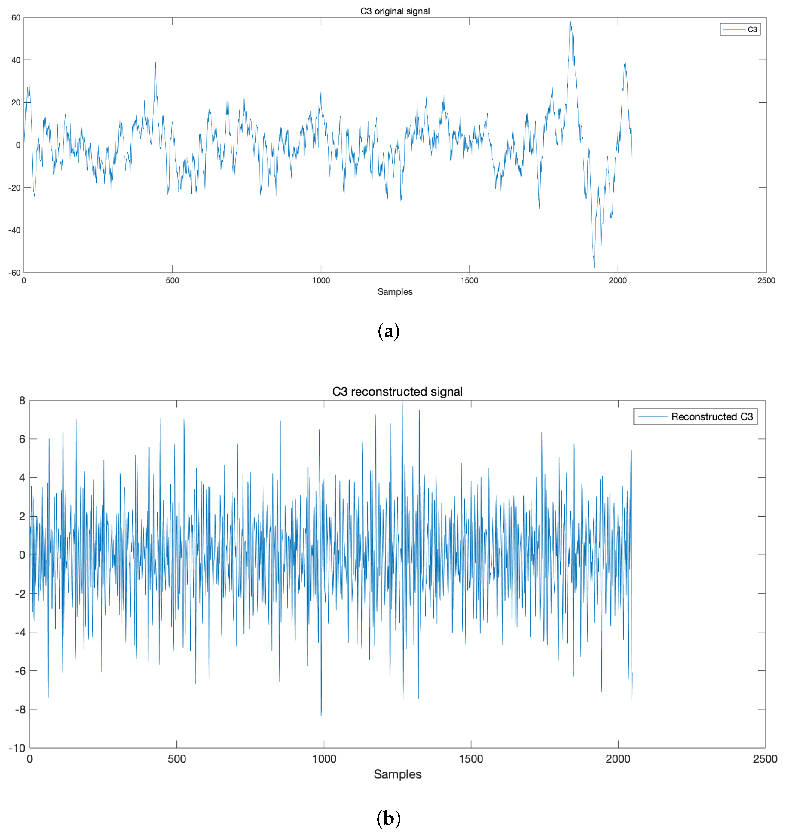
3.2. Denoise Process
3.3. Data Alignment
3.4. Feature Extraction
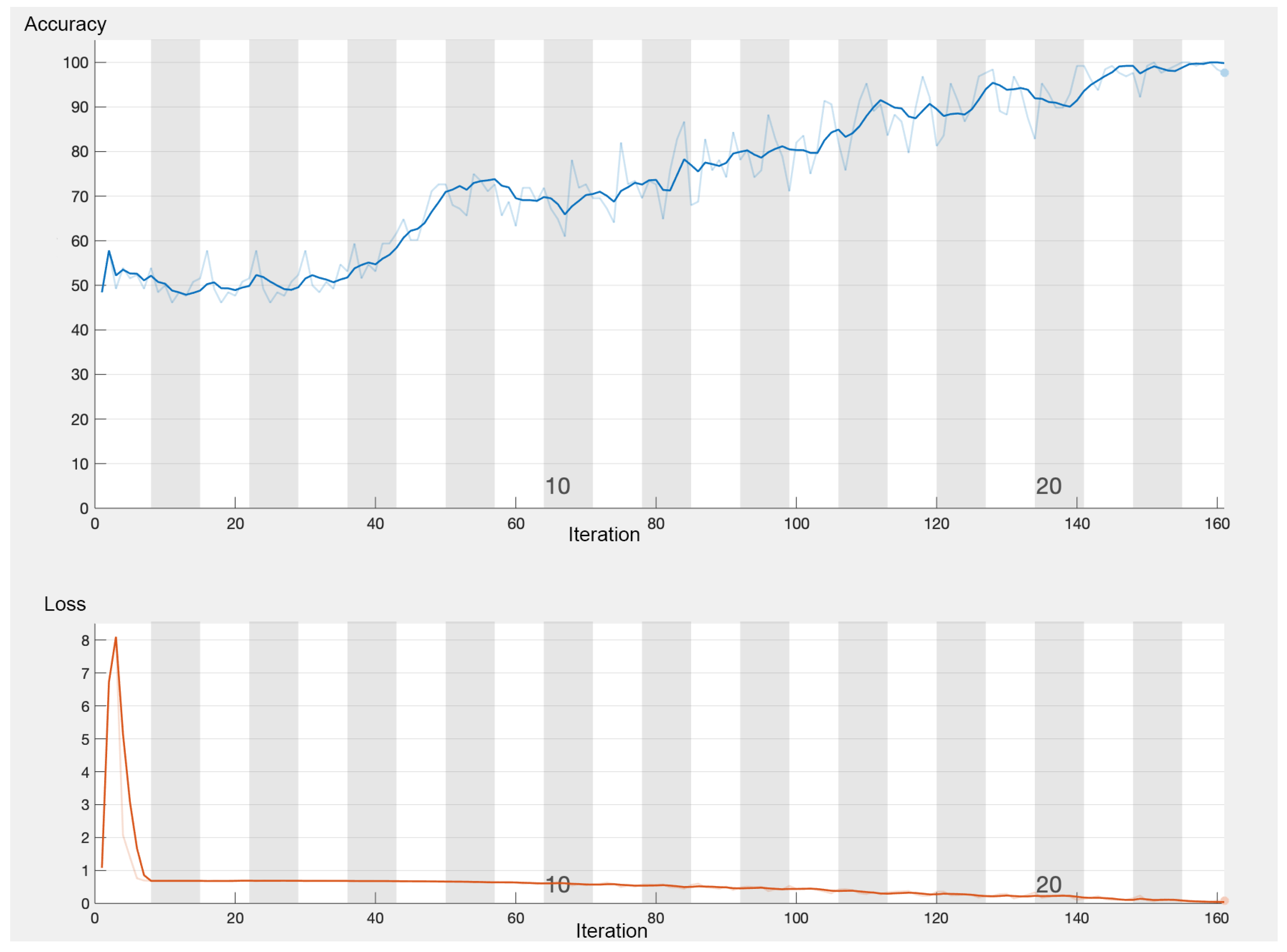
3.5. Pattern Classification
3.6. Comparison Methods
3.7. Results Discussion
4. Conclusions
Author Contributions
Funding
Institutional Review Board Statement
Informed Consent Statement
Data Availability Statement
Conflicts of Interest
References
- Kee, C.Y.; Ponnambalam, S.G.; Loo, C.K. Multi-objective genetic algorithm as channel selection method for P300 and motor imagery data set. Neurocomputing 2015, 161, 120–131. [Google Scholar] [CrossRef]
- Vidal, J.J. Toward direct brain-computer communication. Annu. Rev. Biophys. Bioeng. 1973, 2, 157–180. [Google Scholar] [CrossRef] [PubMed]
- Kotchetkov, I.S.; Hwang, B.Y.; Appelboom, G.; Kellner, C.P.; Connolly, E.S. Brain-computer interfaces: Military, neurosurgical, and ethical perspective. Neurosurg. Focus 2010, 28, E25. [Google Scholar] [CrossRef] [PubMed] [Green Version]
- Huang, M.; Zheng, Y.; Zhang, J.; Guo, B.; Song, C.; Yang, R. Design of a hybrid brain-computer interface and virtual reality system for post-stroke rehabilitation. IFAC-PapersOnLine 2020, 53, 16010–16015. [Google Scholar] [CrossRef]
- Wang, X.; Yang, R.; Huang, M.; Yang, Z.; Wan, Z. A hybrid transfer learning approach for motor imagery classification in brain-computer interface. In Proceedings of the 2021 IEEE 3rd Global Conference on Life Sciences and Technologies, Nara, Japan, 9–11 March 2021; pp. 496–500. [Google Scholar]
- Wei, M.; Yang, R.; Huang, M. Motor imagery EEG signal classification based on deep transfer learning. In Proceedings of the 2021 IEEE 34th International Symposium on Computer-Based Medical Systems, Aveiro, Portugal, 7–9 June 2021; pp. 85–90. [Google Scholar]
- Wan, Z.; Yang, R.; Huang, M.; Liu, W.; Zeng, N. EEG fading data classification based on improved manifold learning with adaptive neighborhood selection. Neurocomputing 2021, 482, 186–196. [Google Scholar] [CrossRef]
- Hinterberger, T.; Kübler, A.; Kaiser, J.; Neumann, N.; Birbaumer, N. A brain–computer interface (BCI) for the locked-in: Comparison of different EEG classifications for the thought translation device. Clin. Neurophysiol. 2003, 114, 416–425. [Google Scholar] [CrossRef]
- Kovari, A. Study of Algorithmic Problem-Solving and Executive Function. Acta Polytech. Hung. 2020, 17, 241–256. [Google Scholar] [CrossRef]
- Kovari, A.; Katona, J.; Costescu, C. Evaluation of eye-movement metrics in a software debbuging task using gp3 eye tracker. Acta Polytech. Hung. 2020, 17, 57–76. [Google Scholar] [CrossRef]
- Kovari, A.; Katona, J.; Costescu, C. Quantitative analysis of relationship between visual attention and eye-hand coordination. Acta Polytech. Hung 2020, 17, 77–95. [Google Scholar] [CrossRef]
- Kovari, A.; Katona, J.; Heldal, I.; Helgesen, C.; Costescu, C.; Rosan, A.; Hathazi, A.; Thill, S.; Demeter, R. Examination of gaze fixations recorded during the trail making test. In Proceedings of the 2019 10th IEEE International Conference on Cognitive Infocommunications (CogInfoCom), Naples, Italy, 23–25 October 2019; pp. 319–324. [Google Scholar]
- Katona, J.; Ujbanyi, T.; Sziladi, G.; Kovari, A. Examine the effect of different web-based media on human brain waves. In Proceedings of the 2017 8th IEEE International Conference on Cognitive Infocommunications (CogInfoCom), Debrecen, Hungary, 11–14 September 2017; pp. 000407–000412. [Google Scholar]
- Costescu, C.; Rosan, A.; Brigitta, N.; Hathazi, A.; Kovari, A.; Katona, J.; Demeter, R.; Heldal, I.; Helgesen, C.; Thill, S.; et al. Assessing Visual Attention in Children Using GP3 Eye Tracker. In Proceedings of the 2019 10th IEEE International Conference on Cognitive Infocommunications (CogInfoCom), Naples, Italy, 23–25 October 2019; pp. 343–348. [Google Scholar] [CrossRef]
- Maravić Čisar, S.; Pinter, R.; Kovári, A.; Pot, M. Application of Eye Movement Monitoring Technique in Teaching Process. IPSI Trans. Adv. Res. 2021, 17, 32–36. [Google Scholar]
- Hamedi, M.; Salleh, S.H.; Noor, A.M. Electroencephalographic motor imagery brain connectivity analysis for BCI: A review. Neural Comput. 2016, 28, 999–1041. [Google Scholar] [CrossRef] [PubMed]
- Schalk, G.; McFarland, D.J.; Hinterberger, T.; Birbaumer, N.; Wolpaw, J.R. BCI2000: A general-purpose brain-computer interface (BCI) system. IEEE Trans. Biomed. Eng. 2004, 51, 1034–1043. [Google Scholar] [CrossRef] [PubMed]
- Richman, J.S.; Moorman, J.R. Physiological time-series analysis using approximate entropy and sample entropy. Am. J. Physiol.-Heart Circ. Physiol. 2000, 278, H2039–H2049. [Google Scholar] [CrossRef] [PubMed] [Green Version]
- Müller-Gerking, J.; Pfurtscheller, G.; Flyvbjerg, H. Designing optimal spatial filters for single-trial EEG classification in a movement task. Clin. Neurophysiol. 1999, 110, 787–798. [Google Scholar] [CrossRef]
- Bashashati, A.; Fatourechi, M.; Ward, R.K.; Birch, G.E. A survey of signal processing algorithms in brain–computer interfaces based on electrical brain signals. J. Neural Eng. 2007, 4, R32–R57. [Google Scholar] [CrossRef] [PubMed] [Green Version]
- Zeiler, M.D.; Fergus, R. Visualizing and understanding convolutional networks. In Proceedings of the European Conference on Computer Vision, Zurich, Switzerland, 6–12 September 2014; Springer: Cham, Switzerland, 2014; pp. 818–833. [Google Scholar]
- Szegedy, C.; Liu, W.; Jia, Y.; Sermanet, P.; Reed, S.; Anguelov, D.; Erhan, D.; Vanhoucke, V.; Rabinovich, A. Going deeper with convolutions. In Proceedings of the IEEE Conference on Computer Vision and Pattern Recognition, Boston, MA, USA, 7–12 June 2015; pp. 1–9. [Google Scholar]
- Guo, X.; Gao, L.; Zhang, S.; Li, Y.; Wu, Y.; Fang, L.; Deng, K.; Yao, Y.; Lian, W.; Wang, R.; et al. Cardiovascular system changes and related risk factors in acromegaly patients: A case-control study. Int. J. Endocrinol. 2015, 2015, 573643. [Google Scholar] [CrossRef] [PubMed]
- Cheng, M.; Gao, X.; Gao, S.; Xu, D. Design and implementation of a brain-computer interface with high transfer rates. IEEE Trans. Biomed. Eng. 2002, 49, 1181–1186. [Google Scholar] [CrossRef]
- Pfurtscheller, G.; Neuper, C.; Guger, C.; Harkam, W.; Ramoser, H.; Schlogl, A.; Obermaier, B.; Pregenzer, M. Current trends in Graz brain-computer interface (BCI) research. IEEE Trans. Rehabil. Eng. 2000, 8, 216–219. [Google Scholar] [CrossRef] [PubMed]
- Haufe, S.; Treder, M.S.; Gugler, M.F.; Sagebaum, M.; Curio, G.; Blankertz, B. EEG potentials predict upcoming emergency brakings during simulated driving. J. Neural Eng. 2011, 8, 056001. [Google Scholar] [CrossRef]
- Wan, Z.; Yang, R.; Huang, M.; Zeng, N.; Liu, X. A review on transfer learning in EEG signal analysis. Neurocomputing 2021, 421, 1–14. [Google Scholar] [CrossRef]
- He, H.; Wu, D. Transfer learning for Brain–Computer interfaces: A Euclidean space data alignment approach. IEEE Trans. Biomed. Eng. 2019, 67, 399–410. [Google Scholar] [CrossRef] [PubMed] [Green Version]
- Koles, Z.J.; Lazar, M.S.; Zhou, S.Z. Spatial patterns underlying population differences in the background EEG. Brain Topogr. 1990, 2, 275–284. [Google Scholar] [CrossRef] [PubMed]
- Russakovsky, O.; Deng, J.; Su, H.; Krause, J.; Satheesh, S.; Ma, S.; Huang, Z.; Karpathy, A.; Khosla, A.; Bernstein, M.; et al. Imagenet large scale visual recognition challenge. Int. J. Comput. Vis. 2015, 115, 211–252. [Google Scholar] [CrossRef] [Green Version]
- Abdel-Hamid, O.; Mohamed, A.R.; Jiang, H.; Deng, L.; Penn, G.; Yu, D. Convolutional neural networks for speech recognition. IEEE/ACM Trans. Audio Speech, Lang. Process. 2014, 22, 1533–1545. [Google Scholar] [CrossRef] [Green Version]
- LeCun, Y.; Boser, B.; Denker, J.S.; Henderson, D.; Howard, R.E.; Hubbard, W.; Jackel, L.D. Backpropagation applied to handwritten zip code recognition. Neural Comput. 1989, 1, 541–551. [Google Scholar] [CrossRef]
- BCI-Horizon. BCI Dataset. 2020. Available online: http://www.bnci-horizon-2020.eu/database/data-sets (accessed on 1 February 2022).
- Pfurtscheller, G.; Neuper, C. Motor imagery and direct brain-computer communication. Proc. IEEE 2001, 89, 1123–1134. [Google Scholar] [CrossRef]
- Maaten, L.v.d.; Hinton, G. Visualizing data using t-SNE. J. Mach. Learn. Res. 2008, 9, 2579–2605. [Google Scholar]


| No | Layer | Options |
|---|---|---|
| 0 | Input EEG | size = (250,250,1) |
| 1 | Convolutional layer | size = (250,250,1), kernel size = (11,11,32), padding = (1,1) |
| 2 | Maxpooling layer | size = (120,120,32), kernel size = (2,2,32), padding = (2,2) |
| 3 | Convolutional layer | size = (110,100,32), kernel size = (11,11,32), padding = (1,1) |
| 4 | Convolutional layer | size = (100,100,32), kernel size = (11,11,32), padding = (1,1) |
| 5 | Maxpooling layer | size = (50,50,32), kernel size = (2,2,32), padding = (2,2) |
| 6 | Convolutional layer | size = (44,44,64), kernel size = (7,7,64), padding = (1,1) |
| 7 | Maxpooling layer | size = (22,22,32), kernel size = (2,2,64), padding = (2,2) |
| 8 | Convolutional layer | size = (20,20,128), kernel size = (3,3,128), padding = (1,1) |
| 9 | Maxpooling layer | size = (10,10,128), kernel size = (2,2,128), padding = (2,2) |
| 10 | Convolutional layer | size = (8,8,128), kernel size = (3,3,128), padding = (1,1) |
| 11 | Maxpooling layer | size = (4,4,128), kernel size = (2,2,128), padding = (2,2) |
| 12 | Fully-Connected layer | size = (2048,1) |
| 13 | Softmax layer | size = 2 |
| Target Subject | EA-CSP-SVM | EA-ftCNN | EA-CSP-CNN |
|---|---|---|---|
| S11 | 69 | 73 | 79 |
| S12 | 72 | 64 | 87 |
| S13 | 74 | 70 | 84 |
| S14 | 60 | 63 | 67 |
Publisher’s Note: MDPI stays neutral with regard to jurisdictional claims in published maps and institutional affiliations. |
© 2022 by the authors. Licensee MDPI, Basel, Switzerland. This article is an open access article distributed under the terms and conditions of the Creative Commons Attribution (CC BY) license (https://creativecommons.org/licenses/by/4.0/).
Share and Cite
Wang, X.; Yang, R.; Huang, M. An Unsupervised Deep-Transfer-Learning-Based Motor Imagery EEG Classification Scheme for Brain–Computer Interface. Sensors 2022, 22, 2241. https://doi.org/10.3390/s22062241
Wang X, Yang R, Huang M. An Unsupervised Deep-Transfer-Learning-Based Motor Imagery EEG Classification Scheme for Brain–Computer Interface. Sensors. 2022; 22(6):2241. https://doi.org/10.3390/s22062241
Chicago/Turabian StyleWang, Xuying, Rui Yang, and Mengjie Huang. 2022. "An Unsupervised Deep-Transfer-Learning-Based Motor Imagery EEG Classification Scheme for Brain–Computer Interface" Sensors 22, no. 6: 2241. https://doi.org/10.3390/s22062241
APA StyleWang, X., Yang, R., & Huang, M. (2022). An Unsupervised Deep-Transfer-Learning-Based Motor Imagery EEG Classification Scheme for Brain–Computer Interface. Sensors, 22(6), 2241. https://doi.org/10.3390/s22062241