
Laboratory Investigation of Tomography-Controlled Continuous Steel Casting

 , , , , , , ,
  , and
, and 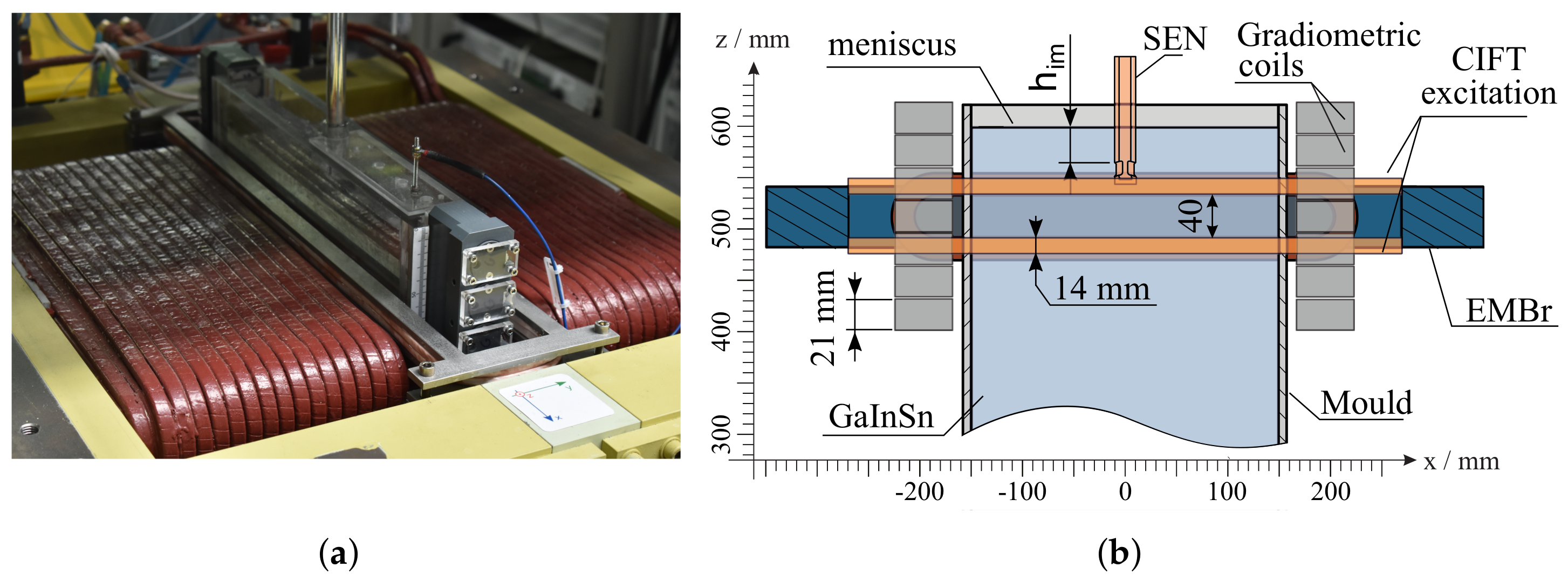
Abstract
:1. Introduction
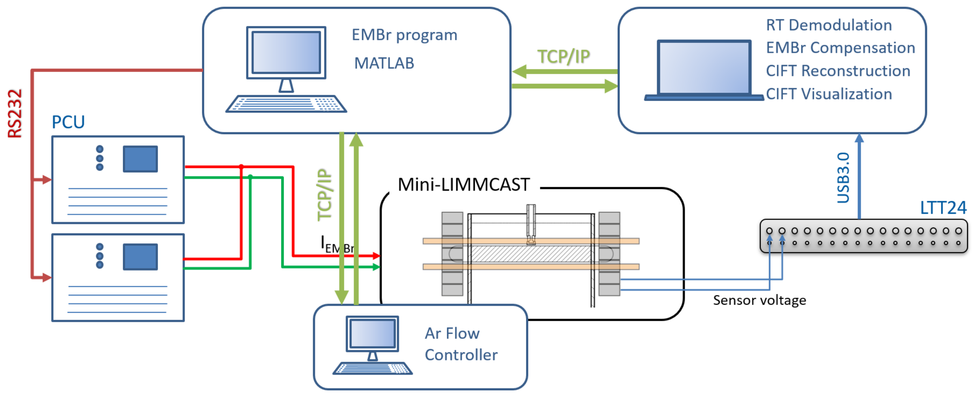
2. Experimental Setup
2.1. Contactless Inductive Flow Tomography
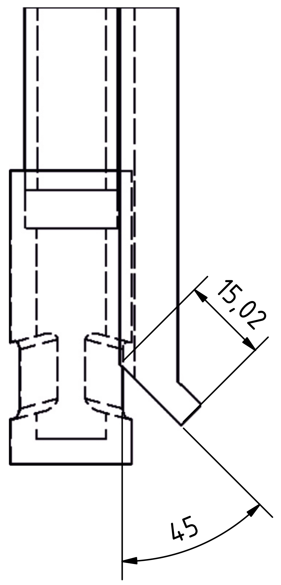
2.2. Mini-LIMMCAST
3. Results
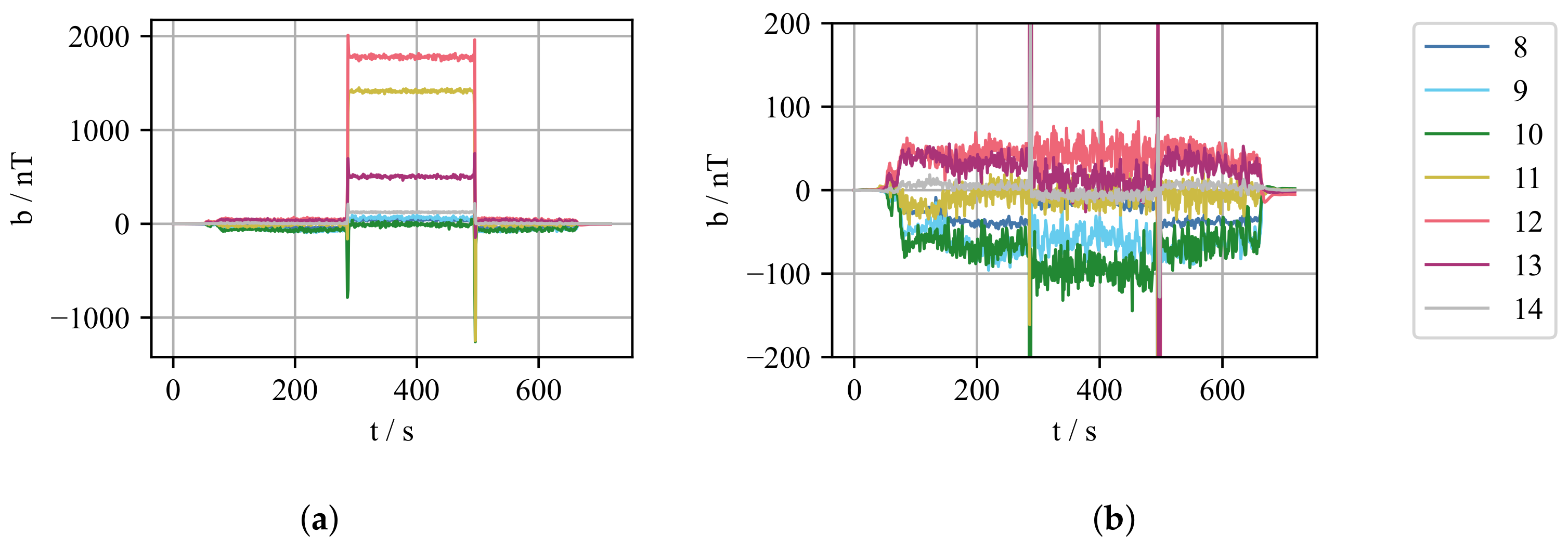
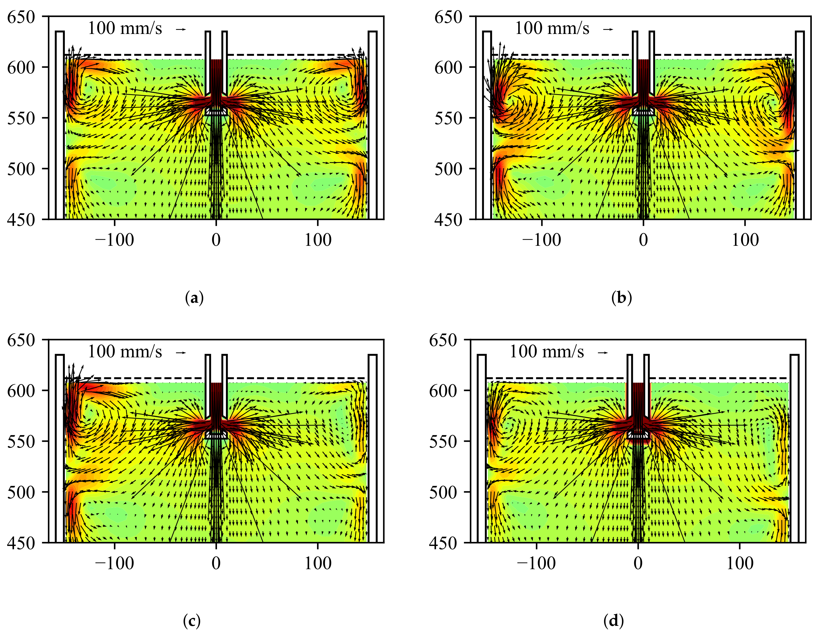
3.1. Effects of the EMBr on CIFT
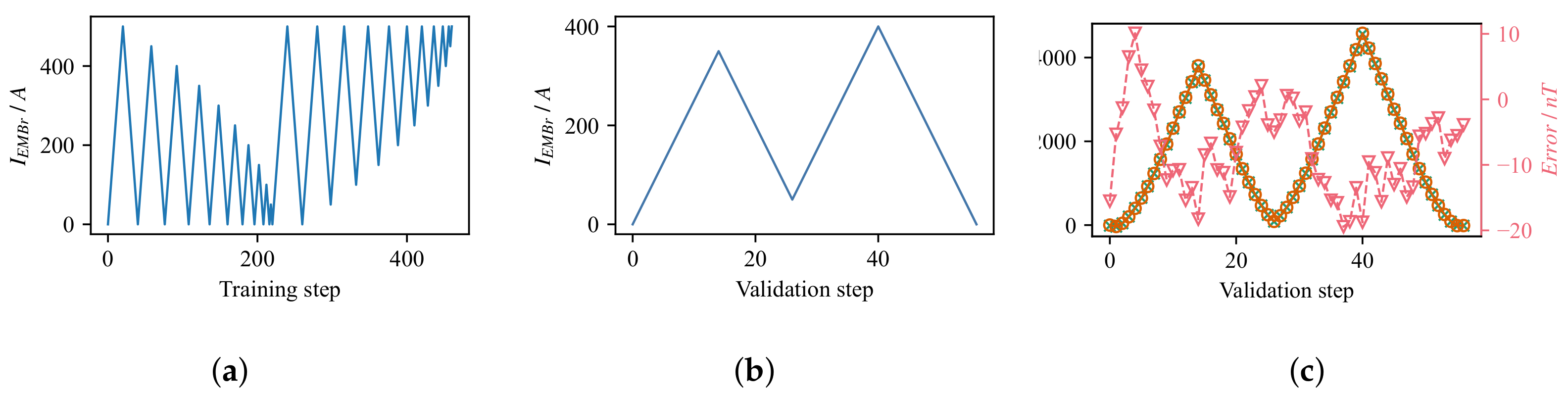
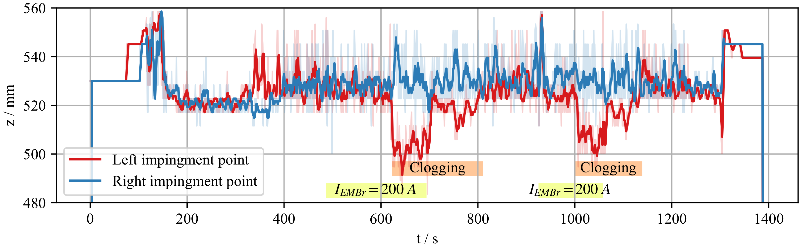
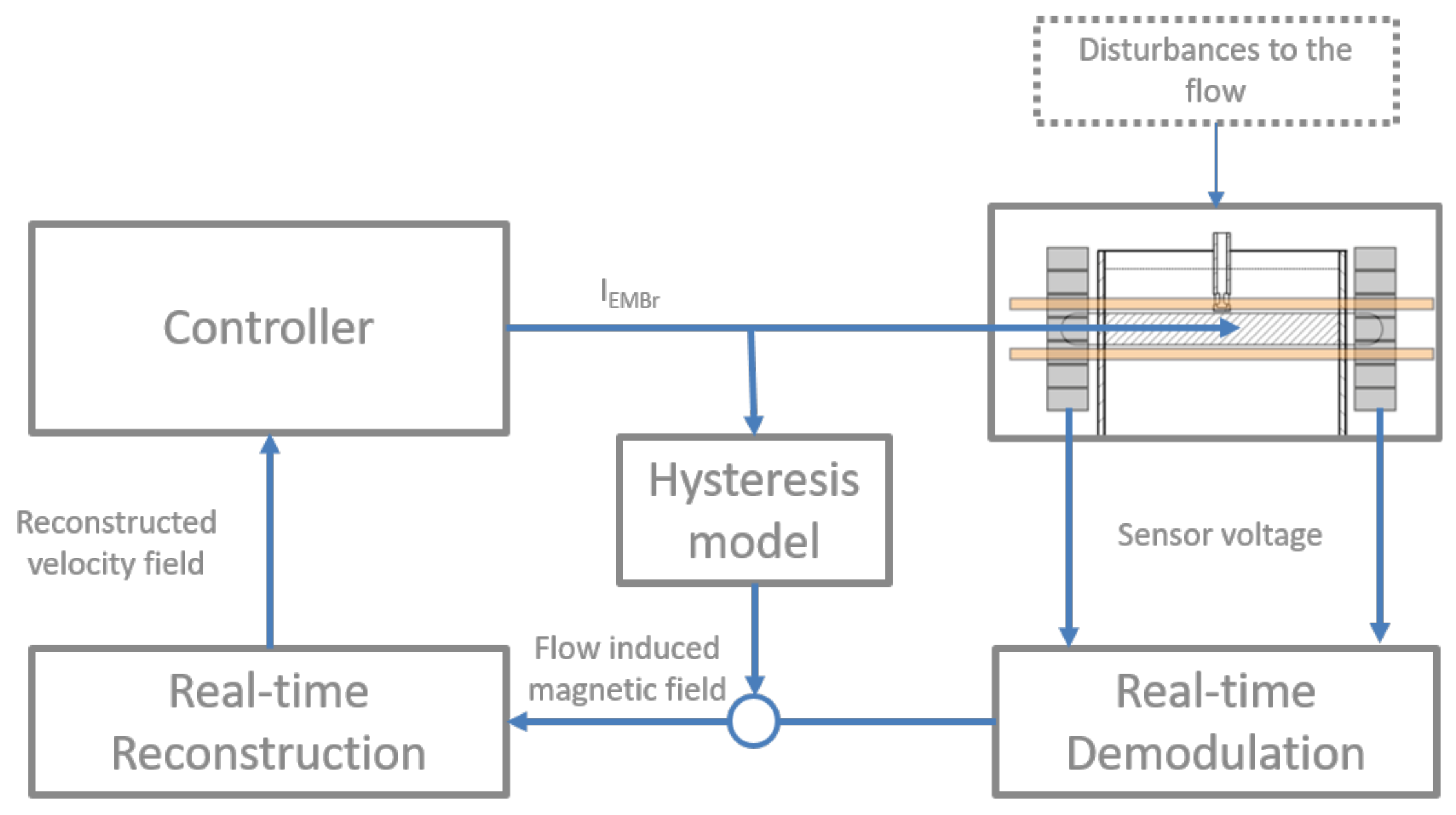
3.2. Control Strategy
4. Conclusions and Outlook
Author Contributions
Funding
Data Availability Statement
Conflicts of Interest
Appendix A

References
- Hibbeler, L.C.; Thomas, B.G. Mold slag entrainment mechanisms in continuous casting molds. In Proceedings of the AISTech 2013, Pittsburgh, PA, USA, 6–9 May 2013. [Google Scholar]
- Thomas, B.G.; Huang, X.; Sussman, R.C. Simulation of Argon Gas Flow Effects in a Continuous Slab Caster. Metall. Mater. Trans. B 1994, 25, 527–547. [Google Scholar] [CrossRef]
- Zhang, L.; Yang, S.; Cai, K.; Li, j.; Wan, X.; Thomas, B.G. Investigation of Fluid Flow and Steel Cleanliness in the Continuous Casting Strand. Metall. Mater. Trans. B 2007, 38, 63–83. [Google Scholar] [CrossRef]
- Cho, S.M.; Thomas, B.G. Electromagnetic Forces in Continuous Casting of Steel Slabs. Metals 2019, 9, 471. [Google Scholar] [CrossRef] [Green Version]
- Thomas, B.G.; Yuan, Q.; Sivaramakrishnan, S.; Shi, T.; Vanka, P.; Assar, M.B. Comparison of four methods to evaluate fluid velocities in a continuous casting mould. Iron Steel Inst. Jpn. Int. 2001, 41, 1181–1193. [Google Scholar] [CrossRef]
- Liu, R.; Thomas, B.G.; Sengupta, J.; Chung, S.D.; Trinh, M. Measurements of Molten Steel Surface Velocity and Effect of Stopper-Rod Movement on Transient Multiphase Fluid Flow in Continuous Casting. ISIJ Int. 2014, 10, 2314–2323. [Google Scholar] [CrossRef] [Green Version]
- Dauby, P.H. Continuous casting: Make better steel and more of it! Rev. MéTallurgie 2012, 109, 113–136. [Google Scholar] [CrossRef]
- Zheng, J.; Runcong, L.; Wang, X.; Xu, G.; Lyu, Z.; Kolesnikov, Y.; Na, X. An online contactless investigation of the meniscus velocity in a continuous casting mould using Lorentz Force Velocimetry. Metall. Mater. B 2020, 41B, 558–569. [Google Scholar]
- Mul, M. Real-time mould temperature control for the purpose of consistent slab quality. In Proceedings of the METEC & 4th ESTAD, Düsseldorf, Germany, 24–28 June 2019. [Google Scholar]
- Hedin, G.; Kamperman, A.; Sedén, M.; Fröjdh, K.; Pejnefors, J. Exploring opportunities in mold temperature monitoring utilizing Fiber Bragg Gratings. In Proceedings of the SCANMET V 2016, Luleå, Sweden, 12–15 June 2016. [Google Scholar]
- Zhang, T.; Yang, J.; Jiang, P. Measurement of Molten Steel Velocity near the Surface and Modeling for Transient Fluid Flow in the Continuous Casting Mold. Metals 2019, 9, 36. [Google Scholar] [CrossRef] [Green Version]
- Hashimoto, Y.; Matsui, A.; Hayase, T.; Kano, M. Real-time estimation of molten steel flow in continuous casting mold. Metall. Mater. B 2020, 51, 581–588. [Google Scholar] [CrossRef]
- Cukierski, K.; Thomas, B.G. Flow Control with Local Electromagnetic Braking in Continuous Casting of Steel Slabs. Metall. Materials Trans. B 2008, 39, 94–107. [Google Scholar] [CrossRef]
- Okazawa, K.; Toh, T.; Fukuda, J.; Kawase, T.; Toki, M. Fluid Flow in a Continuous Casting Mold Driven by Linear Induction Motors. ISIJ Int. 2001, 8, 851–858. [Google Scholar] [CrossRef]
- Schurmann, D.; Glavinić, I.; Willers, B.; Timmel, K.; Eckert, S. Impact of the Electromagnetic Brake Position on the Flow Structure in a Slab Continuous Casting Mold: An Experimental Parameter Study. Metall. Mater. B 2019, 51, 61–78. [Google Scholar] [CrossRef]
- Jin, X.; Chen, F.D.; Zhang, J.; Xie, X.; Bi, Y.Y. Water Model Study on Fluid Flow in Slab Continuous Casting Mould with Solidified Shell. Ironmak. Steelmak. 2011, 38, 155–159. [Google Scholar] [CrossRef]
- Ramirez, L.P.; Bjorkvall, J.; Olofsson, C.; Nazem, J.P.; Sjostrom, U.; Nilsson, C. Continuous casting simulator for measurement and control of liquid metal flow in the mould. In Proceedings of the 8th European Continuous Casting Conference 2014, Graz, Austria, 23–26 June 2014. [Google Scholar]
- Timmel, K.; Eckert, S.; Gerbeth, G.; Stefani, F.; Wondrak, T. Experimental Modeling of the Continuous Casting Process of Steel Using Low Melting Point Metal Alloys—The LIMMCAST Program. ISIJ Int. 2010, 50, 1134–1141. [Google Scholar] [CrossRef] [Green Version]
- Dekemele, K.; Ionescu, C.; De Doncker, M.; De Keyser, R. Closed loop control of an electromagnetic stirrer in the continuous casting process. In Proceedings of the 2016 European Control Conference 2016, Aalborg, Denmark, 29 June–1 July 2016; pp. 61–66. [Google Scholar]
- Watzinger, J.; Watzinger, I. Latest advancements in ESP casting technology. In Proceedings of the European Continous Casting Conference 2021, Bari, Italy, 20–22 October 2021. [Google Scholar]
- Ma, X.; Peyton, A.J.; Higson, S.R.; Lyons, A.; Dickinson, S.J. Hardware and software design for an electromagnetic induction tomography (EMT) system for high contrast metal process applications. Meas. Sci. Technol. 2006, 17, 111. [Google Scholar] [CrossRef]
- Stefani, F.; Gerbeth, G. A contactless method for velocity reconstruction in electrically conducting fluids. Meas. Sci. Technol. 2000, 11, 758–765. [Google Scholar] [CrossRef]
- Terzija, N.; Yin, W.; Gerbeth, G.; Stefani, F.; Timmel, K.; Wondrak, T.; Peyton, A. Electromagnetic inspection of a two-phase flow of GaInSn and Argon. Flow Meas. Instrum. 2011, 22, 10–16. [Google Scholar] [CrossRef]
- Wondrak, T.; Eckert, S.; Gerbeth, G.; Klotsche, K.; Stefani, F.; Timmel, K.; Peyton, A.J.; Terzija, N.; Yin, W. Combined electromagnetic tomography for determining two-phase flow characteristics in the submerged entry nozzle and in the mold of a continuous casting model. Metall. Mater. Trans. B 2011, 42, 1201–1210. [Google Scholar] [CrossRef]
- Muttakin, I.; Soleimani, M. Interior void classification in liquid metal using multi-frequency magnetic induction tomography with a machine learning approach. IEEE Sens. J. 2021, 21, 23289–23296. [Google Scholar] [CrossRef]
- Stefani, F.; Gundrum, T.; Gerbeth, G. Contactless Inductive Flow Tomography. Phys. Rev. E 2004, 5, 056306. [Google Scholar] [CrossRef] [Green Version]
- Wondrak, T.; Galindo, V.; Gerbeth, G.; Gundrum, T.; Stefani, F.; Timmel, K. Contactless inductive flow tomography for a model of continuous steel casting. Meas. Sci. Technol. 2010, 21, 045402. [Google Scholar] [CrossRef]
- Wondrak, T.; Pal, J.; Stefani, F.; Galindo, V.; Eckert, S. Visualization of the global flow structure in a modified Rayleigh-Bénard setup using contactless inductive flow tomography. Flow Meas. Instrum. 2018, 61, 269–280. [Google Scholar] [CrossRef] [Green Version]
- Ratajczak, M.; Wondrak, T.; Stefani, F. A gradiometric version of contactless inductive flow tomography: Theory and first applications. Philos. A 2016, 374, 20150330. [Google Scholar] [CrossRef] [PubMed] [Green Version]
- Ratajczak, M.; Wondrak, T. Analysis, design and optimization of compact ultra-high sensitivity coreless induction coil sensors. Meas. Sci. Technol. 2020, 31, 065902. [Google Scholar] [CrossRef]
- Ratajczak, M.; Wondrak, T.; Timmel, K.; Stefani, F.; Eckert, S. Flow Visualization by Means of Contactless Inductive Flow Tomography in the Presence of a Magnetic Brake. J. Manuf. Sci. Prod. 2015, 15, 41–48. [Google Scholar] [CrossRef]
- Ratajczak, M.; Wondrak, T.; Stefani, F.; Eckert, S. Numerical and experimental investigation of the contactless inductive flow tomography in the presence of strong static magnetic fields. Magnetohydrodynamics 2015, 51, 461–471. [Google Scholar] [CrossRef]
- Glavinić, I.; Stefani, F.; Eckert, S.; Wondrak, T. Real time flow control during continuous casting with contactless inductive flow tomography. In Proceedings of the 10th International Conference on Electromagnetic Processing of Materials 2021, Riga, Latvia, 14–16 June 2021; pp. 170–175. [Google Scholar]
- Wondrak, T.; Jacobs, R.T.; Faber, P. Fast reconstruction algorithm for contactless inductive flow tomography. In Proceedings of the 10th International Conference on Advanced Computer Information Technologies 2020, Deggendorf, Germany, 16–18 September 2020; pp. 217–220. [Google Scholar]
- Abouelazayem, S.; Glavinić, I.; Wondrak, T.; Hlava, J. Flow Control Based on Feature Extraction in Continuous Casting Process. Sensors 2020, 20, 6880. [Google Scholar] [CrossRef]
- Lomb, N.R. Least-square frequency analysis of unequally spaced data. Astrophys. Space Sci. 1976, 39, 447–462. [Google Scholar] [CrossRef]
- Mayergoyz, I.D. Mathematical Models of Hysteresis. Phys. Rev. Lett. 1986, 22, 1518–1521. [Google Scholar] [CrossRef] [Green Version]
- Krasnosel’skiǐ, M.A.; Pokrovskiǐ, A.V. Systems with Hysteresis; Springer: Berlin/Heidelberg, Germany, 1989. [Google Scholar]
- Stakvik, J.Å.; Ragazzon, R.P.M.; Eielsen, A.A.; Gravdahl, J.T. On Implementation of the Preisach Model: Identification and Inversion for Hysteresis Compensation. Model. Identif. Control. Nor. Res. Bull. 2015, 3, 133–142. [Google Scholar] [CrossRef] [Green Version]
- Cho, S.M.; Kim, S.H.; Chaudhary, R.; Thomas, B.G.; Shin, H.J.; Choi, W.R.; Kim, S.K. Effect of nozzle clogging on surface flow and vortex formation in the continuous casting mold. In Proceedings of the AISTech 2011, Indianapolis, IN, USA, 2–5 May 2011. [Google Scholar]
- Hang, C.C.; Astrom, K.J.; Wang, Q.G. Relay Feedback Auto-Tuning of Process Controllers—A Tutorial Review. J. Process. Control 2002, 1, 143–162. [Google Scholar] [CrossRef]


Publisher’s Note: MDPI stays neutral with regard to jurisdictional claims in published maps and institutional affiliations. |
© 2022 by the authors. Licensee MDPI, Basel, Switzerland. This article is an open access article distributed under the terms and conditions of the Creative Commons Attribution (CC BY) license (https://creativecommons.org/licenses/by/4.0/).
Share and Cite
Glavinić, I.; Muttakin, I.; Abouelazayem, S.; Blishchik, A.; Stefani, F.; Eckert, S.; Soleimani, M.; Saidani, I.; Hlava, J.; Kenjereš, S.; et al. Laboratory Investigation of Tomography-Controlled Continuous Steel Casting. Sensors 2022, 22, 2195. https://doi.org/10.3390/s22062195
Glavinić I, Muttakin I, Abouelazayem S, Blishchik A, Stefani F, Eckert S, Soleimani M, Saidani I, Hlava J, Kenjereš S, et al. Laboratory Investigation of Tomography-Controlled Continuous Steel Casting. Sensors. 2022; 22(6):2195. https://doi.org/10.3390/s22062195
Chicago/Turabian StyleGlavinić, Ivan, Imamul Muttakin, Shereen Abouelazayem, Artem Blishchik, Frank Stefani, Sven Eckert, Manuchehr Soleimani, Iheb Saidani, Jaroslav Hlava, Saša Kenjereš, and et al. 2022. "Laboratory Investigation of Tomography-Controlled Continuous Steel Casting" Sensors 22, no. 6: 2195. https://doi.org/10.3390/s22062195
APA StyleGlavinić, I., Muttakin, I., Abouelazayem, S., Blishchik, A., Stefani, F., Eckert, S., Soleimani, M., Saidani, I., Hlava, J., Kenjereš, S., & Wondrak, T. (2022). Laboratory Investigation of Tomography-Controlled Continuous Steel Casting. Sensors, 22(6), 2195. https://doi.org/10.3390/s22062195