
Detection and Mosaicing Techniques for Low-Quality Retinal Videos

 ,
,  ,
,  and
and 
Abstract
:1. Introduction
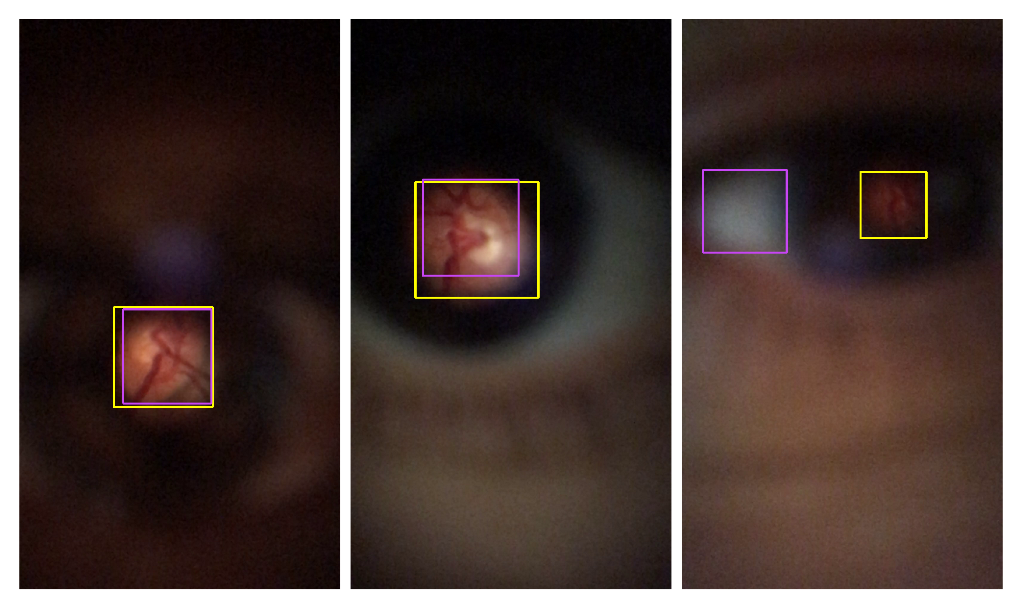
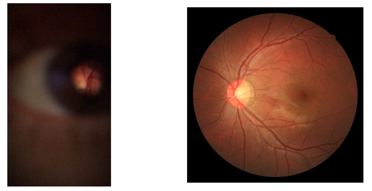
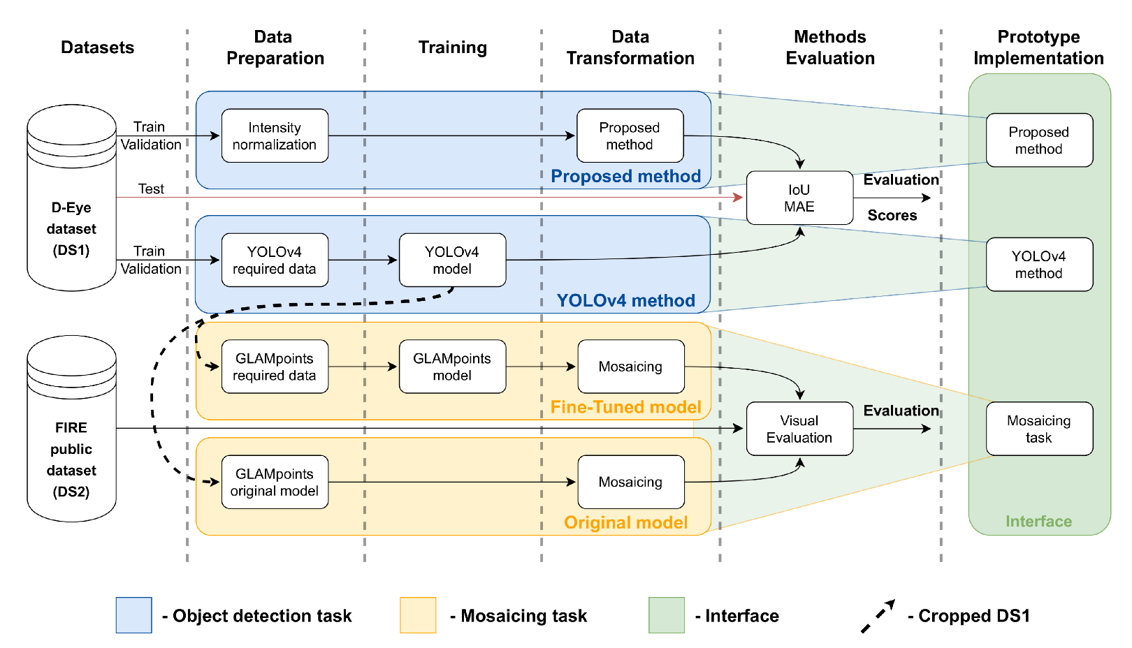
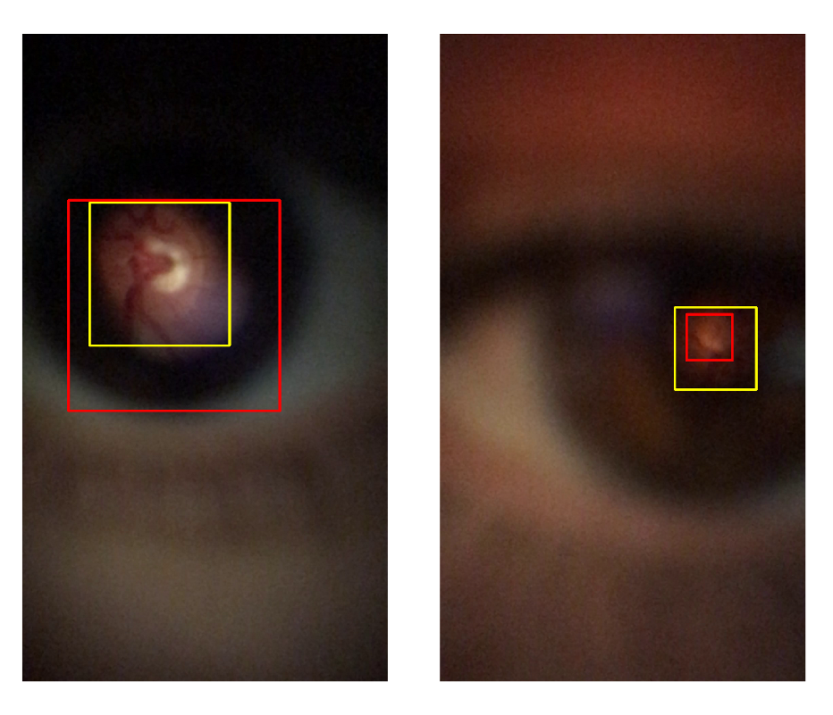
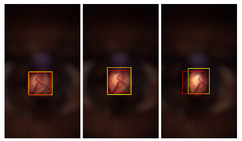
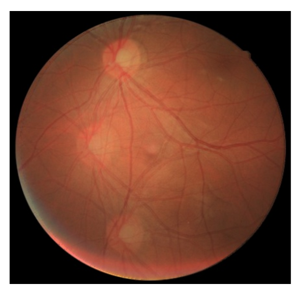
- The first task is a framework focused on the detection of lower-resolution retinal images taken with a smartphone equipped with a D-Eye lens. Here, two methods were proposed and compared: a classical image processing approach and a YOLO v4 neural network. To explore this task, a private dataset presented by Zengin et al. [6], which contains 26 retina videos around the optic disc, with lower-resolution images, and annotated two subsets, one with the localization of the visible retinal area and other with vessel segmentation was used;
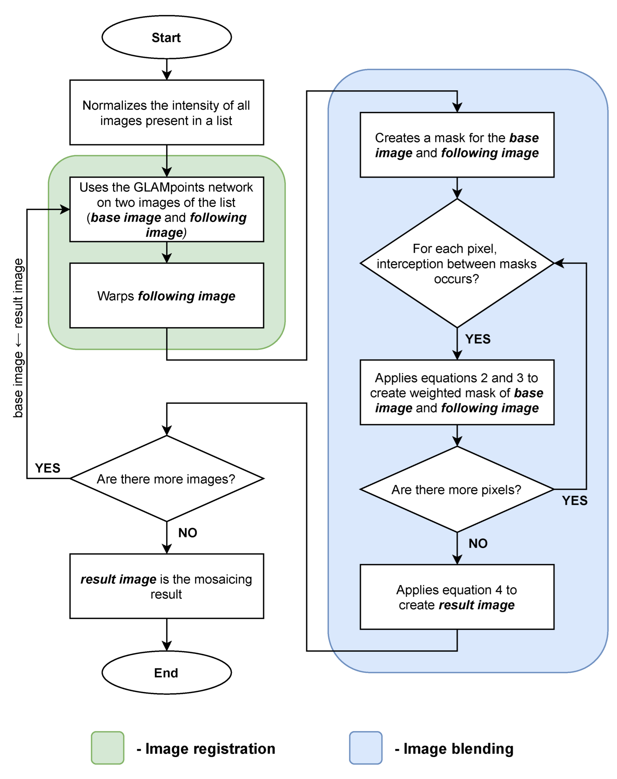
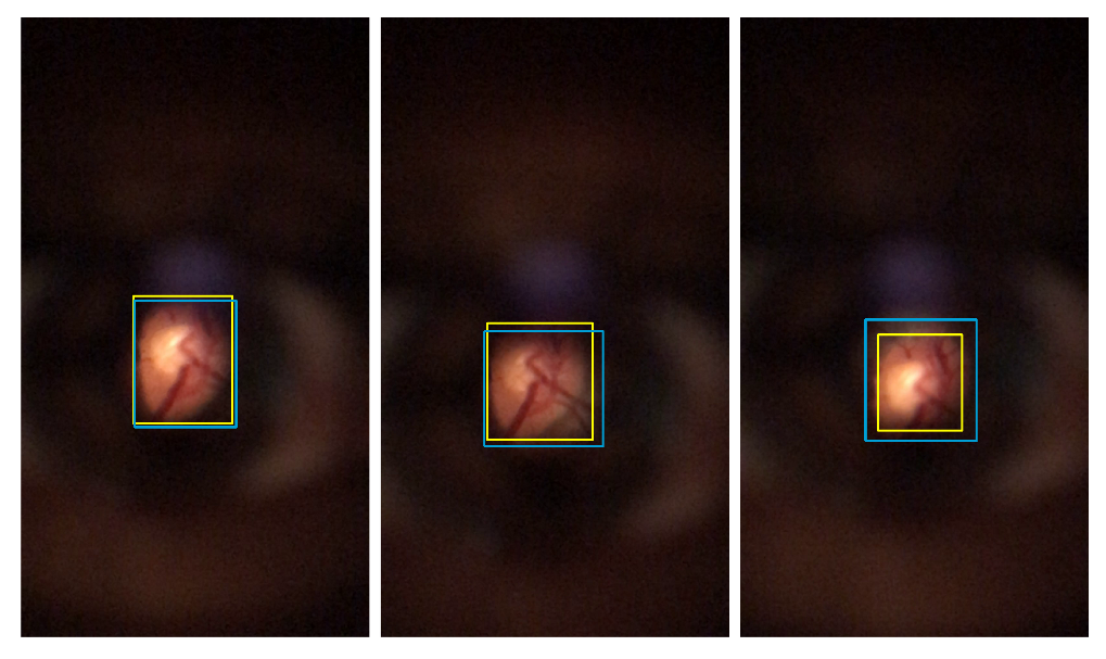
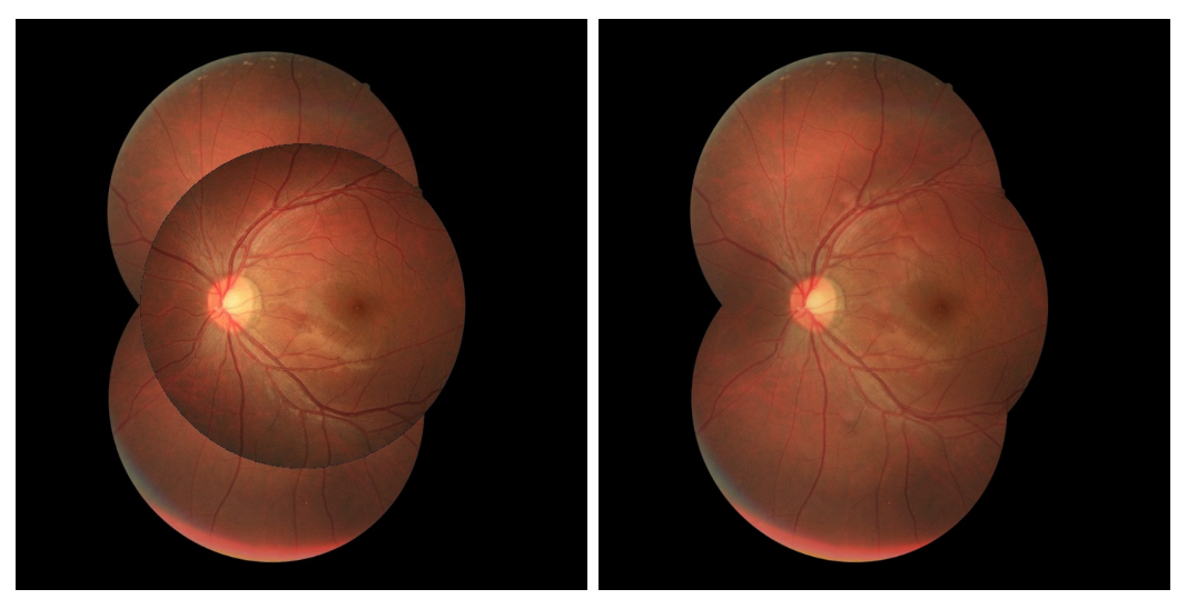
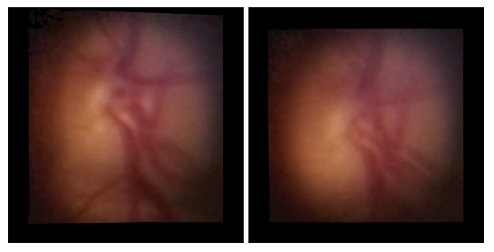
- The second task explored in this paper is the mosaicing technique in images captured from devices attached with D-Eye lenses so that a summary image can be provided as the result of some retinal video. It was explored the Glampoints model proposed by Truong et al. [7] applied to the images resulting from the previously described task.
2. Related Work
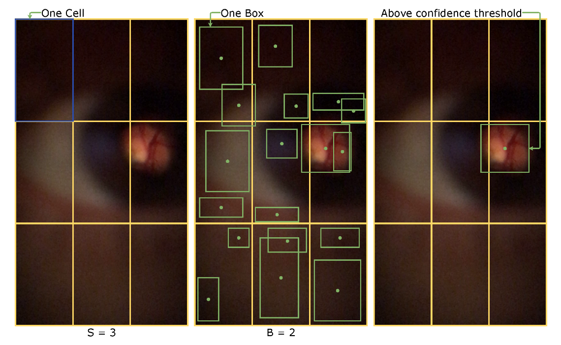
2.1. Object Detection
- is the number of columns/rows which the image is divided;
- x, y are the center coordinates of the bounding box;
- h, w are the height and width, respectively, of the bounding box. These values fluctuate from 0 to 1 as a ratio of the image height or width;
- pc is the confidence score, the probability of a bounding box contains an object;
- B is the number of bounding box that each cell contains;
- C is the number of classes that the model is trained to detect. Will return the probability of each cell contains an object.
2.2. Mosaicing
3. Materials and Methods
3.1. Datasets
3.2. Data Preparation
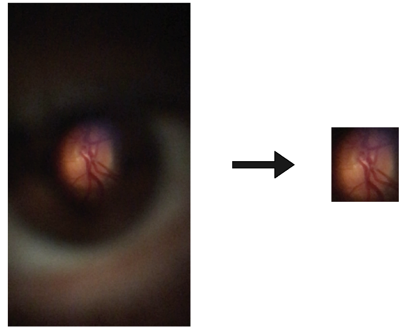
3.2.1. Proposed Method
3.2.2. Yolo V4 Network
3.2.3. Mosaicing
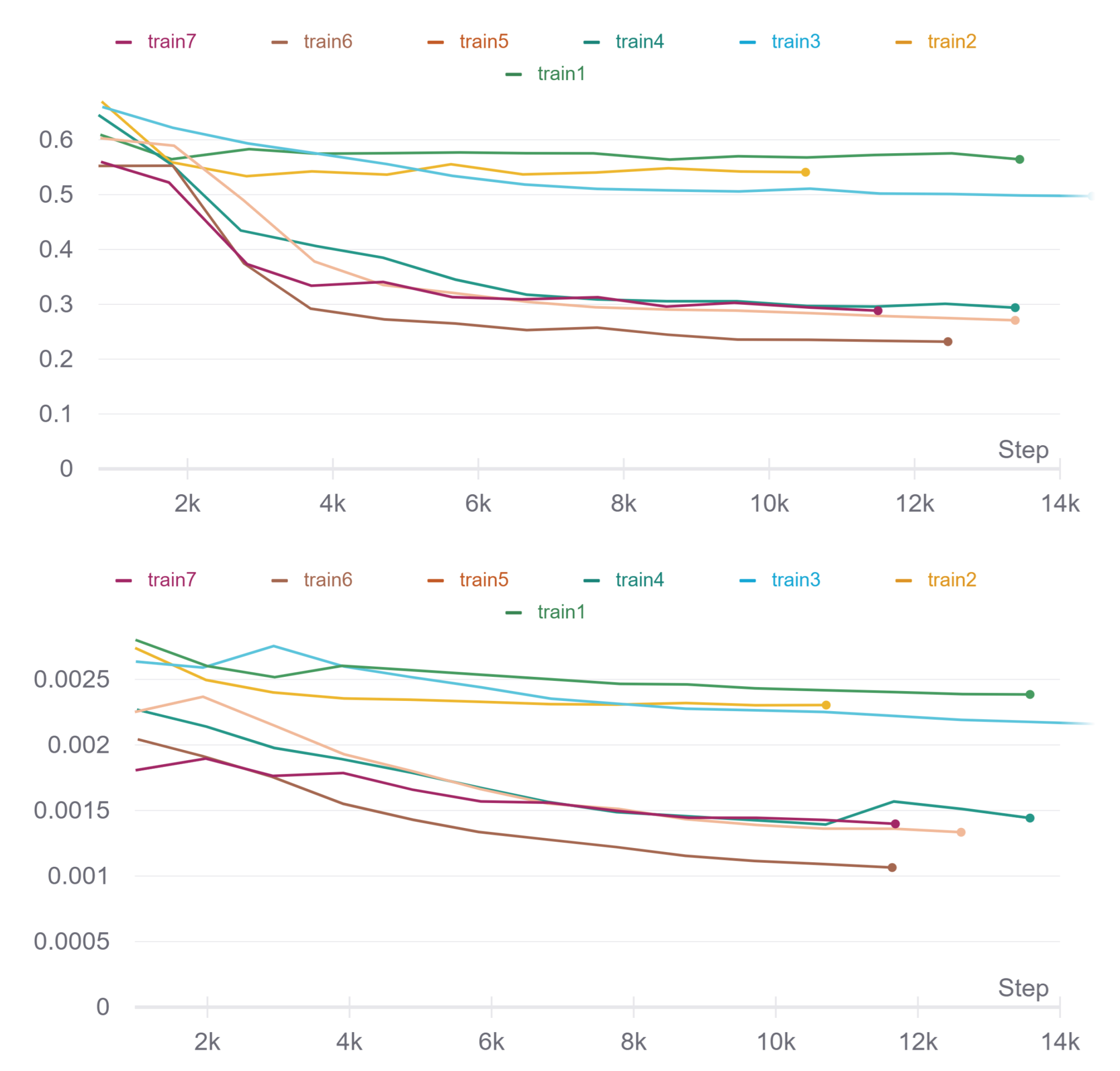
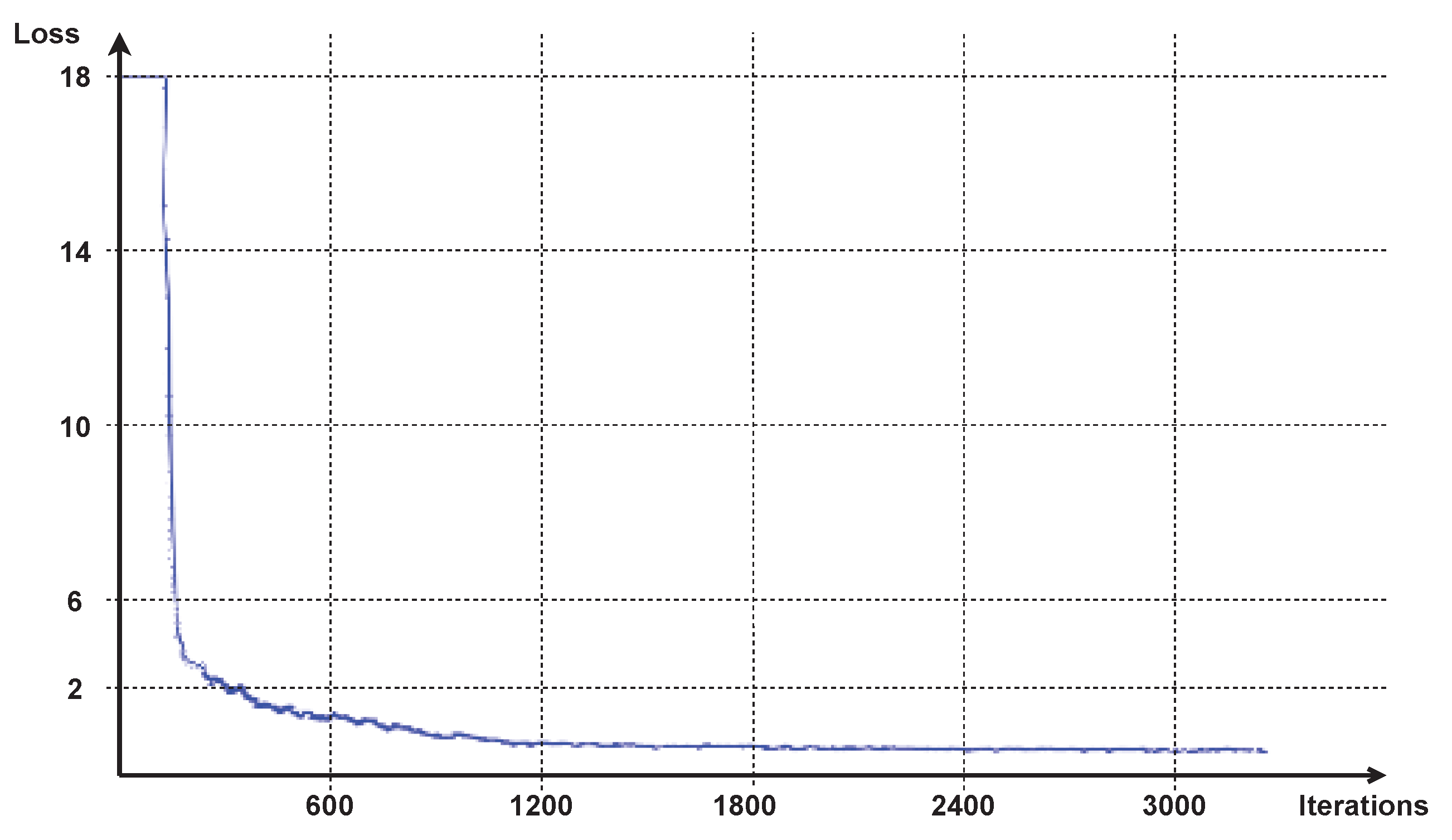
3.3. Training
3.4. Data Transformation
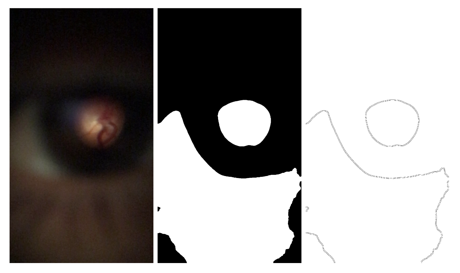
3.4.1. Proposed Method
3.4.2. Mosaicing
3.5. Evaluation
4. Results and Discussion
4.1. Retinal Detection
4.2. Mosaicing
5. Conclusions
Author Contributions
Funding
Institutional Review Board Statement
Informed Consent Statement
Data Availability Statement
Acknowledgments
Conflicts of Interest
Abbreviations
| BB | Bounding Box |
| CHT | Circle Hough Transform |
| FOV | Field of View |
| IoU | Intersection over Union |
| MAE | Mean Absolute Error |
| RoI | Region of Interest |
| SIFT | Scale-invariant feature transform |
| YOLO | You Only Look Once |
References
- Russo, A.; Morescalchi, F.; Costagliola, C.; Delcassi, L.; Semeraro, F. A novel device to exploit the smartphone camera for fundus photography. J. Ophthalmol. 2015, 2015, 1–5. [Google Scholar] [CrossRef] [PubMed]
- Maamari, R.N.; Keenan, J.D.; Fletcher, D.A.; Margolis, T.P. A mobile phone-based retinal camera for portable wide field imaging. Br. J. Ophthalmol. 2014, 98, 438–441. [Google Scholar] [CrossRef] [PubMed]
- Inview®. Available online: https://www.volk.com/collections/diagnostic-imaging/products/inview-for-iphone-6-6s.html (accessed on 26 February 2021).
- Wu, A.R.; Fouzdar-Jain, S.; Suh, D.W. Comparison study of funduscopic examination using a smartphone-based digital ophthalmoscope and the direct ophthalmoscope. J. Pediatr. Ophthalmol. Strabismus 2018, 55, 201–206. [Google Scholar] [CrossRef] [PubMed]
- Hernandez-Matas, C.; Zabulis, X.; Triantafyllou, A.; Anyfanti, P.; Douma, S.; Argyros, A.A. FIRE: Fundus image registration dataset. J. Model. Ophthalmol. 2017, 1, 16–28. [Google Scholar] [CrossRef]
- Zengin, H.; Camara, J.; Coelho, P.; Rodrigues, J.M.; Cunha, A. Low-Resolution Retinal Image Vessel Segmentation. In Proceedings of the International Conference on Human-Computer Interaction, Copenhagen, Denmark, 19–24 July 2020; Springer: Berlin/Heidelberg, Germany, 2020; pp. 611–627. [Google Scholar]
- Truong, P.; Apostolopoulos, S.; Mosinska, A.; Stucky, S.; Ciller, C.; Zanet, S.D. GLAMpoints: Greedily Learned Accurate Match points. In Proceedings of the IEEE International Conference on Computer Vision, Seoul, Korea, 27–28 October 2019; pp. 10732–10741. [Google Scholar]
- Liu, L.; Ouyang, W.; Wang, X.; Fieguth, P.; Chen, J.; Liu, X.; Pietikäinen, M. Deep learning for generic object detection: A survey. Int. J. Comput. Vis. 2020, 128, 261–318. [Google Scholar] [CrossRef] [Green Version]
- Jiao, L.; Zhang, F.; Liu, F.; Yang, S.; Li, L.; Feng, Z.; Qu, R. A survey of deep learning-based object detection. IEEE Access 2019, 7, 128837–128868. [Google Scholar] [CrossRef]
- Redmon, J.; Divvala, S.; Girshick, R.; Farhadi, A. You only look once: Unified, real-time object detection. In Proceedings of the IEEE Conference on Computer Vision and Pattern Recognition, Las Vegas, NV, USA, 27–30 June 2016; pp. 779–788. [Google Scholar]
- Patton, N.; Aslam, T.M.; MacGillivray, T.; Deary, I.J.; Dhillon, B.; Eikelboom, R.H.; Yogesan, K.; Constable, I.J. Retinal image analysis: Concepts, applications and potential. Prog. Retin. Eye Res. 2006, 25, 99–127. [Google Scholar] [CrossRef] [PubMed]
- Melo, T.; Mendonça, A.M.; Campilho, A. Creation of Retinal Mosaics for Diabetic Retinopathy Screening: A Comparative Study. In Proceedings of the International Conference Image Analysis and Recognition, Póvoa de Varzim, Portugal, 27–29 June 2018; Springer: Berlin/Heidelberg, Germany, 2018; pp. 669–678. [Google Scholar]
- Ghosh, D.; Kaabouch, N. A survey on image mosaicing techniques. J. Vis. Commun. Image Represent. 2016, 34, 1–11. [Google Scholar] [CrossRef]
- Lin, T.Y.; Maire, M.; Belongie, S.; Hays, J.; Perona, P.; Ramanan, D.; Dollár, P.; Zitnick, C.L. Microsoft Coco: Common objects in context. In Proceedings of the European conference on Computer Vision, Zurich, Switzerland, 6–12 September 2014; Springer: Berlin/Heidelberg, Germany, 2014; pp. 740–755. [Google Scholar]
- WandB. Available online: http://www.wandb.ai (accessed on 20 September 2021).
- Kimme, C.; Ballard, D.; Sklansky, J. Finding circles by an array of accumulators. Commun. ACM 1975, 18, 120–122. [Google Scholar] [CrossRef]
- Otsu, N. A threshold selection method from gray-level histograms. IEEE Trans. Syst. Man. Cybern. 1979, 9, 62–66. [Google Scholar] [CrossRef] [Green Version]
- Willmott, C.J.; Matsuura, K. Advantages of the mean absolute error (MAE) over the root mean square error (RMSE) in assessing average model performance. Clim. Res. 2005, 30, 79–82. [Google Scholar] [CrossRef]
- Zhou, D.; Fang, J.; Song, X.; Guan, C.; Yin, J.; Dai, Y.; Yang, R. IoU loss for 2d/3d object detection. In Proceedings of the 2019 International Conference on 3D Vision (3DV), Québec City, QC, Canada, 15–18 September 2019; pp. 85–94. [Google Scholar]


| Resolution (Pixels) | Train | Validation | Test | |
|---|---|---|---|---|
| DS1 | 1920 × 1080 | 18 videos; 3881 images | 3 videos; 776 images | 5 videos; 1375 images |
| Resolution (Pixels) | S Category | P Category | A Category | |
|---|---|---|---|---|
| DS2 | 2912 × 2912 | 71 pairs | 49 pairs | 14 pairs |
| Name | Use Green Channel | Use Rotation | Use Scaling | Use Perspective | Use Shearing |
|---|---|---|---|---|---|
| Train 1 | no | yes | yes | yes | yes |
| Train 2 | no | yes | yes | yes | yes |
| Train 3 | no | no | yes | yes | yes |
| Train 4 | no | no | no | yes | yes |
| Train 5 | no | no | no | no | yes |
| Train 6 | no | no | yes | yes | no |
| Train 7 | yes | no | no | yes | yes |
| SUCCESSFUL (IoU > 0.8) | ACCEPTABLE (0.6 <IoU ≤ 0.8) | FAILED (IoU ≤ 0.6) | ||||||||||
|---|---|---|---|---|---|---|---|---|---|---|---|---|
| Frequency | MAE | IoU | Frequency | MAE | IoU | Frequency | MAE | IoU | ||||
| Absolute | Relative | Absolute | Relative | Absolute | Relative | |||||||
| Zengin et al. [6] | 615 | 44.73% | 12.84 | 0.85 | 544 | 39.56% | 26.69 | 0.73 | 216 | 15.71% | 80.27 | 0.48 |
| Proposed method | 562 | 40.87% | 13.52 | 0.85 | 627 | 45.60% | 26.24 | 0.73 | 186 | 13.53% | 73.99 | 0.48 |
| YOLO v4 | 1075 | 78.18% | 11.05 | 0.88 | 299 | 21.75% | 25.73 | 0.75 | 1 | 0.07% | 40.25 | 0.60 |
| Mean | Standard Deviation | ||
|---|---|---|---|
| Zengin et al. [6] | MAE | 28.91 | 47.04 |
| IoU | 0.75 | 0.14 | |
| Proposed method | MAE | 27.5 | 29.29 |
| IoU | 0.75 | 0.13 | |
| YOLO v4 | MAE | 14.26 | 7.92 |
| IoU | 0.85 | 0.07 |
Publisher’s Note: MDPI stays neutral with regard to jurisdictional claims in published maps and institutional affiliations. |
© 2022 by the authors. Licensee MDPI, Basel, Switzerland. This article is an open access article distributed under the terms and conditions of the Creative Commons Attribution (CC BY) license (https://creativecommons.org/licenses/by/4.0/).
Share and Cite
Camara, J.; Silva, B.; Gouveia, A.; Pires, I.M.; Coelho, P.; Cunha, A. Detection and Mosaicing Techniques for Low-Quality Retinal Videos. Sensors 2022, 22, 2059. https://doi.org/10.3390/s22052059
Camara J, Silva B, Gouveia A, Pires IM, Coelho P, Cunha A. Detection and Mosaicing Techniques for Low-Quality Retinal Videos. Sensors. 2022; 22(5):2059. https://doi.org/10.3390/s22052059
Chicago/Turabian StyleCamara, José, Bruno Silva, António Gouveia, Ivan Miguel Pires, Paulo Coelho, and António Cunha. 2022. "Detection and Mosaicing Techniques for Low-Quality Retinal Videos" Sensors 22, no. 5: 2059. https://doi.org/10.3390/s22052059
APA StyleCamara, J., Silva, B., Gouveia, A., Pires, I. M., Coelho, P., & Cunha, A. (2022). Detection and Mosaicing Techniques for Low-Quality Retinal Videos. Sensors, 22(5), 2059. https://doi.org/10.3390/s22052059