
Towards On-Device Dehydration Monitoring Using Machine Learning from Wearable Device’s Data

 , , , , and
Abstract
:
1. Introduction
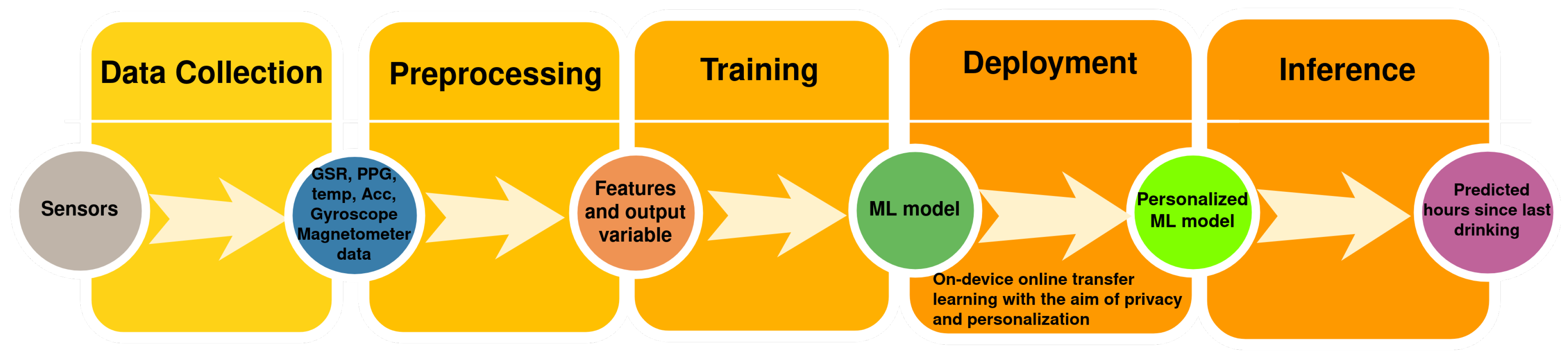
- We propose modeling the dehydration problem as a regression problem to predict the last drinking time using features extracted and constructed from multiple wearable sensors (accelerometer, magnetometer, gyroscope, galvanic skin response (GSR) sensor, photoplethysmography (PPG) sensor, temperature, and barometric pressure sensor);
- For this purpose, we recorded a total of 3386 min for these sensors for 11 subjects under fasting and non-fasting conditions;
- We compared different machine learning models for this task according to four metrics that evaluated the accuracy of the model, training time, and model size and for on-device personalization optimization through the transfer learning experiment;
- A comparison to the state-of-art research for this task was performed. Challenges and limitations were discussed, and further research directions were highlighted.
2. Background and Related Work
2.1. Dehydration Detection
2.2. On-Device Machine Learning
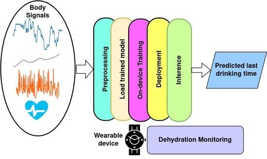
3. Machine Learning for Dehydration Monitoring
4. Dataset, Preprocessing, and Feature Extraction
4.1. Sensors’ Data Preprocessing
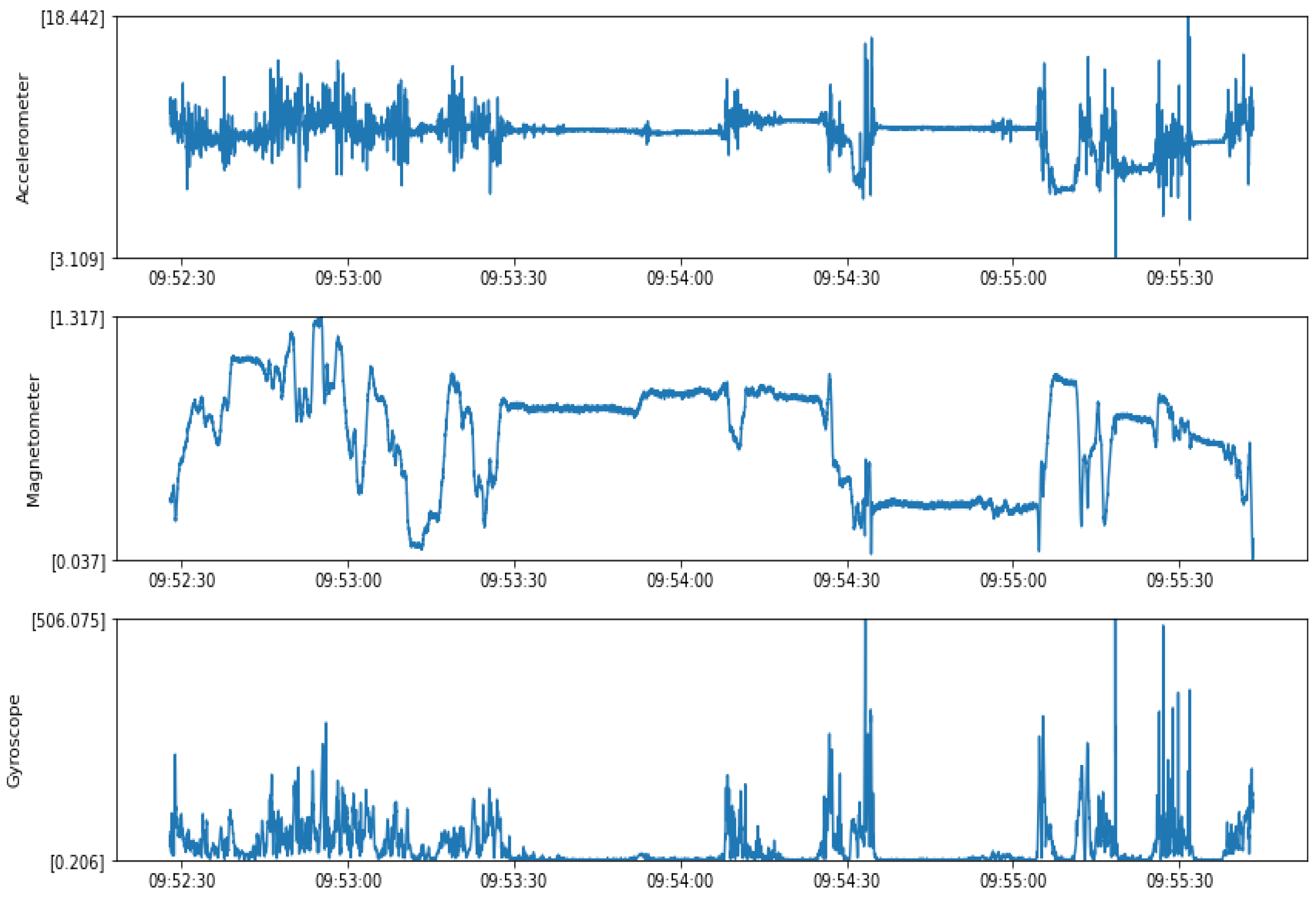
4.1.1. Accelerometer Data
4.1.2. Magnetometer Data
4.1.3. Gyroscope Data
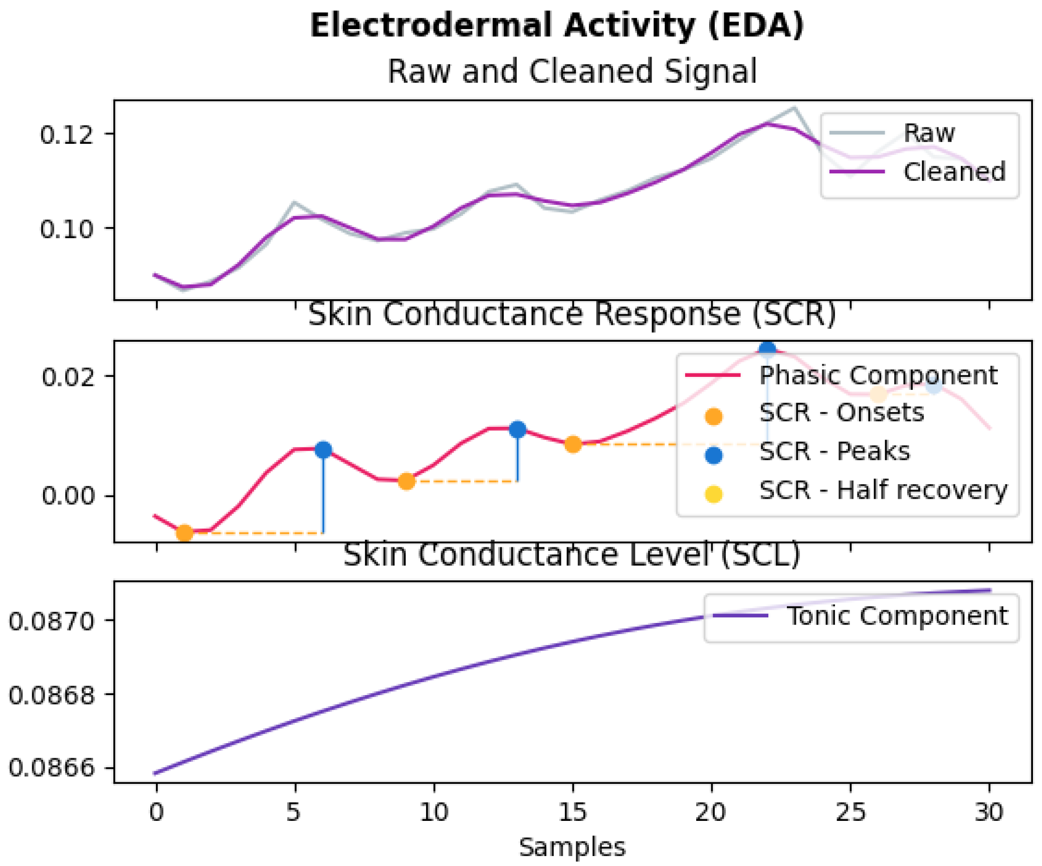
4.1.4. GSR Data
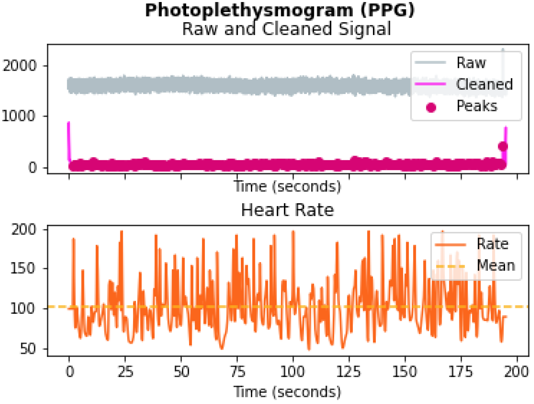
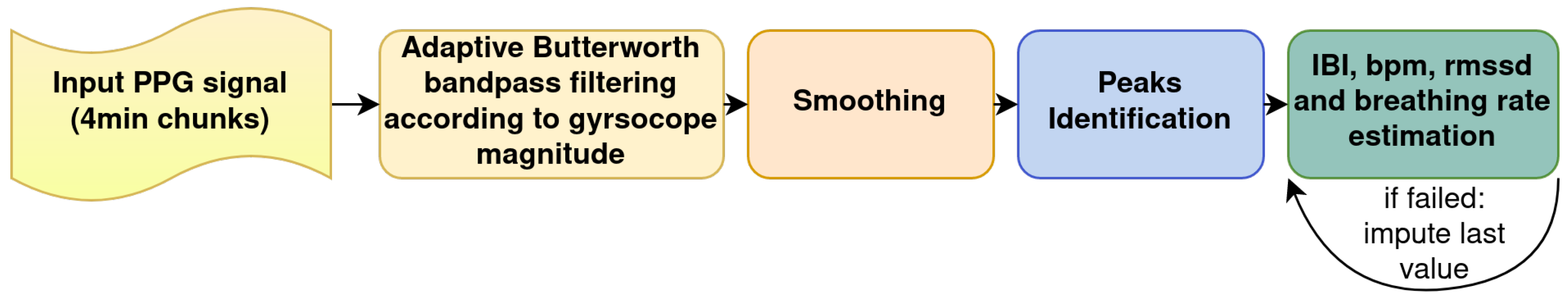
4.1.5. PPG Data
4.1.6. Temperature and Pressure Data
4.2. Descriptive Statistics
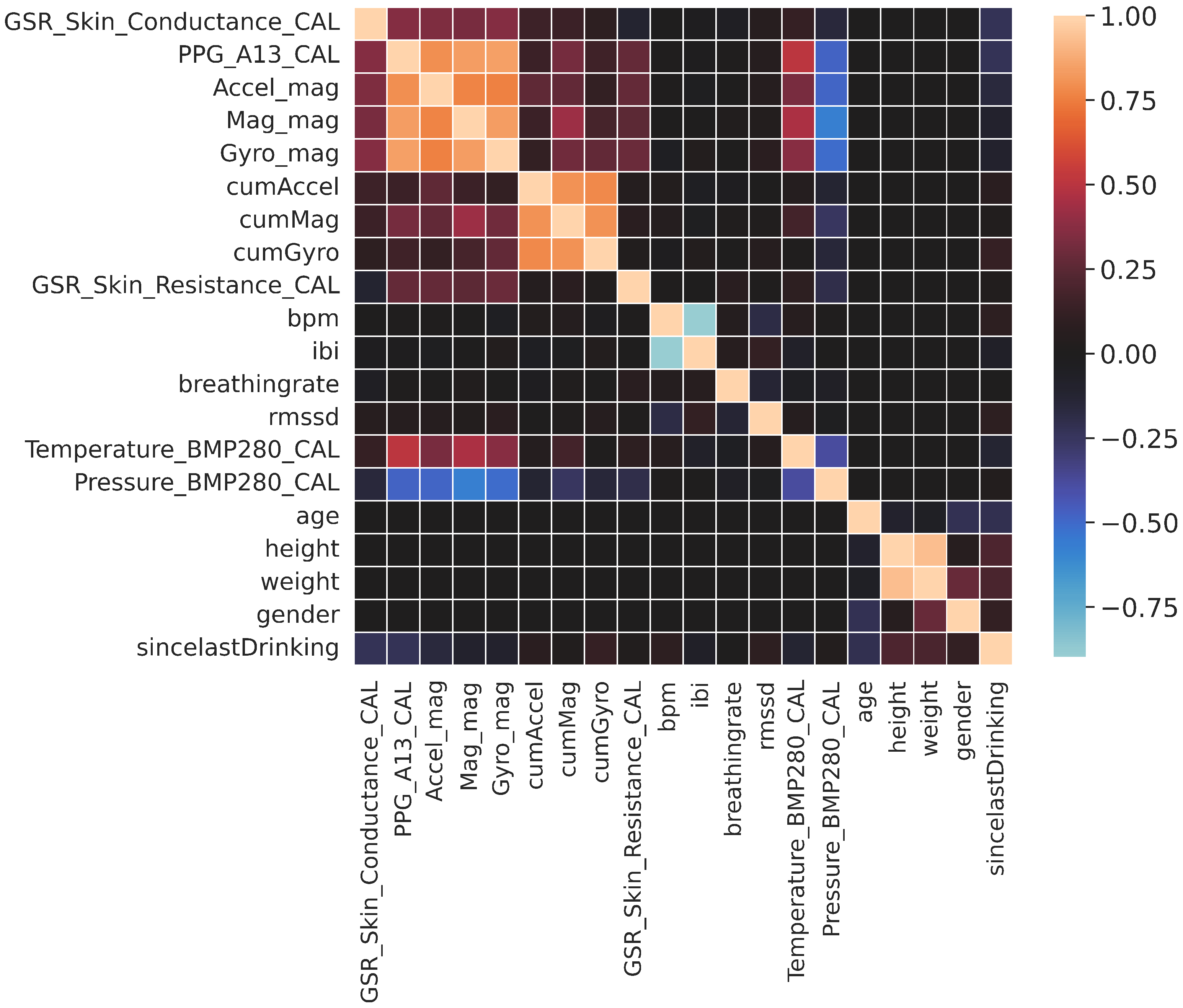
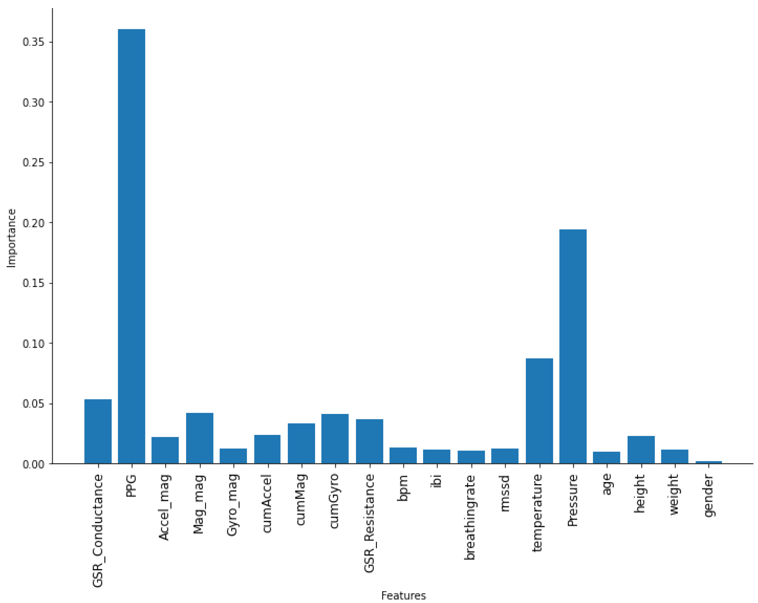
4.3. Features
5. Results
6. Discussion
7. Conclusions
Author Contributions
Funding
Institutional Review Board Statement
Informed Consent Statement
Data Availability Statement
Acknowledgments
Conflicts of Interest
Abbreviations
| ACC | Accelerometer magnitude |
| AI | Artificial intelligence |
| BMI | Body mass index |
| CNN | Convolutional neural network |
| DNN | Deep neural network |
| ECG | Electrocardiogram |
| EDA | Electrodermal activity |
| FEAT1 | Set of 20 features in Table 2 |
| FEAT2 | Set of 12 aggregated and summarized features in Section 4.3 |
| GSR | Galvanic skin response |
| GYRO | Gyroscope magnitude |
| HAR | Human activity recognition |
| HRV | Heart rate variability |
| IBI | Inter-beat interval |
| IRB | Institutional Review Board |
| KNN | K-nearest neighbor |
| LDA | Linear discriminant analysis |
| LR | Linear regression |
| MAE | Mean absolute error |
| MAG | Magnetometer magnitude |
| PPG | Photoplethysmography |
| QDA | Quadratic discriminant analysis |
| RMSE | Root-mean-squared error |
| RMSSD | Root mean sum of squares of the differences between adjacent RR-intervals |
| SVM | Support vector machine |
| SVR | Support vector regression |
| SDRR | Standard deviation of RR-interval |
| VIF | Variance inflation factor |
Appendix A. Specification of the Device Sensors’ Used for Data Collection

| Source | STMicro LSM303DLHC |
| Range | +/−16 g |
| Channels | 3 Channels (x, y, z) |
| Sampling Rate | 512 Hz |
| Filtering | None |
| Source | STMicro LSM303DLHC |
| Range | +/−1.9 Ga |
| Channels | 3 Channels (x, y, z) |
| Sampling Rate | 512 Hz |
| Filtering | None |
| Source | Invensense MPU9150 |
| Range | +/−500 deg/s |
| Channels | 3 Channels (x, y, z) |
| Sampling Rate | 512 Hz |
| Filtering | None |
| Channels | 1 Channel (GSR) |
| Sampling Rate | 128 Hz |
| Format | 16 bits, signed |
| Units | kOhms |
| Filtering | None |
| Channels | 1 Channel (PPG) |
| Sampling Rate | 128 Hz |
| Format | 16 bits, signed |
| Units | mV |
| Filtering | None |
References
- Toral, V.; García, A.; Romero, F.J.; Morales, D.P.; Castillo, E.; Parrilla, L.; Gómez-Campos, F.M.; Morillas, A.; Sánchez, A. Wearable System for Biosignal Acquisition and Monitoring Based on Reconfigurable Technologies. Sensors 2019, 19, 1590. [Google Scholar] [CrossRef] [PubMed] [Green Version]
- Athavale, Y.; Krishnan, S. Biosignal monitoring using wearables: Observations and opportunities. Biomed. Signal Process. Control. 2017, 38, 22–33. [Google Scholar] [CrossRef]
- Military Nutrition Research Institute. Nutritional Needs in Cold and in High-Altitude Environments: Applications for Military Personnel in Field Operations; National Academies Press: Washington, DC, USA, 1996. [Google Scholar]
- Liaqat, S.; Dashtipour, K.; Arshad, K.; Ramzan, N. Non Invasive Skin Hydration Level Detection Using Machine Learning. Electronics 2020, 9, 1086. [Google Scholar] [CrossRef]
- Bell, B.; Alam, R.; Alshurafa, N. Automatic, wearable-based, in-field eating detection approaches for public health research: A scoping review. NPJ Digit. Med. 2020, 3, 38. [Google Scholar] [CrossRef] [Green Version]
- Rizwan, A.; Abu Ali, N.; Zoha, A.; Ozturk, M.; Alomainy, A.; Imran, M.A.; Abbasi, Q.H. Non-Invasive Hydration Level Estimation in Human Body Using Galvanic Skin Response. IEEE Sens. J. 2020, 20, 4891–4900. [Google Scholar] [CrossRef] [Green Version]
- Posada-Quintero, H.; Reljin, N.; Moutran, A.; Georgopalis, D.; Lee, E.; Giersch, G.; Casa, D.; Chon, K. Mild Dehydration Identification Using Machine Learning to Assess Autonomic Responses to Cognitive Stress. Nutrients 2019, 12, 42. [Google Scholar] [CrossRef] [Green Version]
- Dhar, S.; Guo, J.; Liu, J.J.; Tripathi, S.; Kurup, U.; Shah, M. A Survey of On-Device Machine Learning: An Algorithms and Learning Theory Perspective. ACM Trans. Internet Things 2021, 2, 15. [Google Scholar] [CrossRef]
- Kairouz, P.; McMahan, H.B.; Avent, B.; Bellet, A.; Bennis, M.; Bhagoji, A.N.; Bonawitz, K.; Charles, Z.; Cormode, G.; Cummings, R.; et al. Advances and Open Problems in Federated Learning. arXiv 2019, arXiv:1912.04977. [Google Scholar]
- Ghaffari, R.; Rogers, J.A.; Ray, T.R. Recent progress, challenges, and opportunities for wearable biochemical sensors for sweat analysis. Sens. Actuators B Chem. 2021, 332, 129447. [Google Scholar] [CrossRef]
- Ray, T.; Choi, J.; Reeder, J.; Lee, S.P.; Aranyosi, A.J.; Ghaffari, R.; Rogers, J.A. Soft, skin-interfaced wearable systems for sports science and analytics. Curr. Opin. Biomed. Eng. 2019, 9, 47–56. [Google Scholar] [CrossRef]
- Besler, B.C.; Fear, E.C. Microwave Hydration Monitoring: System Assessment Using Fasting Volunteers. Sensors 2021, 21, 6949. [Google Scholar] [CrossRef] [PubMed]
- Mengistu, Y.; Pham, M.; Manh Do, H.; Sheng, W. AutoHydrate: A wearable hydration monitoring system. In Proceedings of the 2016 IEEE/RSJ International Conference on Intelligent Robots and Systems (IROS), Daejeon, Korea, 9–14 October 2016; pp. 1857–1862. [Google Scholar] [CrossRef]
- Alvarez, A.; Severeyn, E.; Velásquez, J.; Wong, S.; Perpiñan, G.; Huerta, M. Machine Learning Methods in the Classification of the Athletes Dehydration. In Proceedings of the 2019 IEEE Fourth Ecuador Technical Chapters Meeting (ETCM), Guayaquil, Ecuador, 11–15 November 2019; pp. 1–5. [Google Scholar] [CrossRef]
- Kulkarni, N.; Compton, C.; Luna, J.; Alam, M.A.U. A Non-Invasive Context-Aware Dehydration Alert System. In Proceedings of the HotMobile ’21: The 22nd International Workshop on Mobile Computing Systems and Applications, Virtual Event, 24–26 February 2021; Association for Computing Machinery: New York, NY, USA, 2021; pp. 157–159. [Google Scholar] [CrossRef]
- Ray, P.P. A review on TinyML: State-of-the-art and prospects. J. King Saud Univ. Comput. Inf. Sci. 2021; in press. [Google Scholar] [CrossRef]
- Cai, H.; Gan, C.; Zhu, L.; Han, S. TinyTL: Reduce Memory, Not Parameters for Efficient On-Device Learning. In Advances in Neural Information Processing Systems; Larochelle, H., Ranzato, M., Hadsell, R., Balcan, M.F., Lin, H., Eds.; Curran Associates, Inc.: Red Hook, NY, USA, 2020; Volume 33, pp. 11285–11297. [Google Scholar]
- Woodward, K.; Kanjo, E.; Brown, D.J.; McGinnity, T.M. On-Device Transfer Learning for Personalising Psychological Stress Modelling using a Convolutional Neural Network. arXiv 2020, arXiv:2004.01603. [Google Scholar]
- Gudur, G.K.; Sundaramoorthy, P.; Umaashankar, V. ActiveHARNet: Towards On-Device Deep Bayesian Active Learning for Human Activity Recognition. In Proceedings of the EMDL ’19: The 3rd International Workshop on Deep Learning for Mobile Systems and Applications, Seoul, Korea, 21 June 2019; Association for Computing Machinery: New York, NY, USA, 2019; pp. 7–12. [Google Scholar] [CrossRef]
- Segev, N.; Harel, M.; Mannor, S.; Crammer, K.; El-Yaniv, R. Learn on Source, Refine on Target: A Model Transfer Learning Framework with Random Forests. IEEE Trans. Pattern Anal. Mach. Intell. 2017, 39, 1811–1824. [Google Scholar] [CrossRef] [Green Version]
- Hamäläinen, W.; Järvinen, M.; Martiskainen, P.; Mononen, J. Jerk-based feature extraction for robust activity recognition from acceleration data. In Proceedings of the 2011 11th International Conference on Intelligent Systems Design and Applications, Córdoba, Spain, 22–24 November 2011; pp. 831–836. [Google Scholar] [CrossRef]
- Pan, Y.C.; Goodwin, B.M.; Sabelhaus, E.; Peters, K.M.; Bjornson, K.F.; Pham, K.; Walker, W.; Steele, K.M. Feasibility of using acceleration-derived jerk to quantify bimanual arm use. J. NeuroEng. Rehabil. 2020, 17, 4768–4777. [Google Scholar] [CrossRef] [Green Version]
- Ode, K.L.; Shi, S.; Katori, M.; Mitsui, K.; Takanashi, S.; Oguchi, R.; Aoki, D.; Ueda, H.R. A jerk-based algorithm ACCEL for the accurate classification of sleep–wake states from arm acceleration. iScience 2022, 25, 103727. [Google Scholar] [CrossRef]
- Olivas-Padilla, B.E.; Manitsaris, S.; Menychtas, D.; Glushkova, A. Stochastic-Biomechanic Modeling and Recognition of Human Movement Primitives, in Industry, Using Wearables. Sensors 2021, 21, 2497. [Google Scholar] [CrossRef]
- Affanni, A. Wireless Sensors System for Stress Detection by Means of ECG and EDA Acquisition. Sensors 2020, 20, 2026. [Google Scholar] [CrossRef] [Green Version]
- Greco, A.; Valenza, G.; Scilingo, E.P. Advances in Electrodermal Activity Processing with Applications for Mental Health, 1st ed.; Springer International Publishing: New York, NY, USA, 2016. [Google Scholar] [CrossRef] [Green Version]
- Posada-Quintero, H.F.; Chon, K.H. Innovations in Electrodermal Activity Data Collection and Signal Processing: A Systematic Review. Sensors 2020, 20, 479. [Google Scholar] [CrossRef] [Green Version]
- Beach, C.; Li, M.; Balaban, E.; Casson, A.J. Motion artefact removal in electroencephalography and electrocardiography by using multichannel inertial measurement units and adaptive filtering. Healthc. Technol. Lett. 2021, 8, 128–138. [Google Scholar] [CrossRef]
- van Gent, P.; Farah, H.; van Nes, N.; van Arem, B. HeartPy: A novel heart rate algorithm for the analysis of noisy signals. Transp. Res. Part F Traffic Psychol. Behav. 2019, 66, 368–378. [Google Scholar] [CrossRef] [Green Version]
- Banbury, C.; Reddi, V.J.; Torelli, P.; Jeffries, N.; Kiraly, C.; Montino, P.; Kanter, D.; Ahmed, S.; Pau, D. MLPerf Tiny Benchmark. In Proceedings of the Thirty-Fifth Conference on Neural Information Processing Systems, Datasets and Benchmarks Track (Round 1), NeurIPS, Virtual Event, 7 December 2021. [Google Scholar]
- Ghassemi, M.; Oakden-Rayner, L.; Beam, A.L. The false hope of current approaches to explainable artificial intelligence in healthcare. Lancet Digit. Health 2021, 3, e745–e750. [Google Scholar] [CrossRef]
- Lundberg, S.M.; Lee, S.I. A Unified Approach to Interpreting Model Predictions. In Proceedings of the NIPS’17: 31st International Conference on Neural Information Processing Systems, Long Beach, CA, USA, 4–9 December 2017; Curran Associates Inc.: Red Hook, NY, USA, 2017; pp. 4768–4777. [Google Scholar]
| Subject | Total Recorded Duration (min) | Maximum Fasting Duration (h) | Mean HR (bpm) | |Accelerometer| (Min., Mean, Max.) (m/s2) | |Magnetometer| (Min., Mean, Max.) (Ga) | |Gyroscope| (Min., Mean, Max.) (deg/s) |
|---|---|---|---|---|---|---|
| S1 | 1768 | 15.3 | 80 | (5.9, 11.9, 27.7) | (0.3, 2.3, 64.7) | (1.5, 25.3, 574.2) |
| S2 | 636 | 13.2 | 67 | (6.4, 10.8, 27.7) | (0.6, 2.7, 71.4) | (1.6, 26.8, 616.3) |
| S3 | 182 | 15 | 86 | (8.1, 11.3, 12.1) | (0.3, 0.9, 1.6) | (2.7, 5.2, 76.9) |
| S4 | 573 | 12.1 | 83 | (8, 11.6, 27.7) | (0.4, 1.8, 53.9) | (1.5, 20.1, 458.1) |
| S5 | 82 | 11 | 81 | (5.8, 11.3, 12.1) | (0.4, 0.9, 1.3) | (1.7, 25.5, 78.6) |
| S6 | 23 | 11.2 | 84 | (9.5, 11.4, 12.3) | (0.4, 0.6, 0.7) | (3.4, 23.9, 57.7) |
| S7 | 24 | 1.4 | 61 | (10.8, 11.9, 12.3) | (0.4, 0.5, 0.8) | (1.7, 4.3, 17.7) |
| S8 | 21 | 1.4 | 81 | (6.9, 8.4, 11) | (0.6, 1, 1.1) | (1.7, 13, 33.2) |
| S9 | 23 | 1.4 | 84 | (10.9, 11.8, 12) | (0.4, 0.6, 0.7) | (1.6, 2.4, 9.6) |
| S10 | 22 | 1.4 | 118 | (10.1, 10.9, 11.3) | (0.6, 0.9, 1) | (8.1, 20.1, 66.3) |
| S11 | 32 | 1.5 | 85 | (10.5, 11.7, 12.3) | (0.4, 0.5, 0.6) | (1.7, 6.4, 27.6) |
| Feature | Description | Mean | VIF |
|---|---|---|---|
| PPG_A13_CAL | Raw PPG sensor calibrated values | 2925 | 5.97 |
| bpm | Estimated pulse rate (beats per minute) | 78 | 5.57 |
| ibi | Inter-beat interval (IBI) estimated from the PPG signal | 772 | 5.53 |
| breathingrate | Estimated breathing rate from the PPG signal | 0.22 | 1.08 |
| RMSSD | Root mean square of successive differences between estimated heartbeats | 75.2 | 1.08 |
| GSR_Skin_Resistance_CAL | Raw calibrated GSR resistance (kOhms) | 9923 | 1.21 |
| GSR_Skin_Conductance_CAL | Raw calibrated GSR conductance (μS) | 5 | 1.31 |
| Accel_mag | Magnitude of the accelerometer, Equation (1) | 11.5 | 5.19 |
| Mag_mag | Magnitude of the magnetometer, Equation (3) | 2 | 7.81 |
| Gyro_mag | Magnitude of the gyroscope, Equation (5) | 22.3 | 7.87 |
| cumAccel | Cumulative accelerometer change, Equation (2) | 2970 | 6.34 |
| cumMag | Cumulative magnetometer change, Equation (4) | 3401 | 7.08 |
| cumGyro | Cumulative gyroscope change, Equation (6) | 46,318 | 6.02 |
| Temperature_BMP280_CAL | Surrounding temperature | 34.9 | 1.53 |
| Pressure_BMP280_CAL | Atmospheric pressure | 99.7 | 1.6 |
| age | Age of the subject | 30 | 1.14 |
| height | Height of the subject (cm) | 159 | 11.23 |
| weight | Weight of the subject (kg) | 63 | 12.11 |
| gender | Gender of the subject (male/female) | N/A | 1.8 |
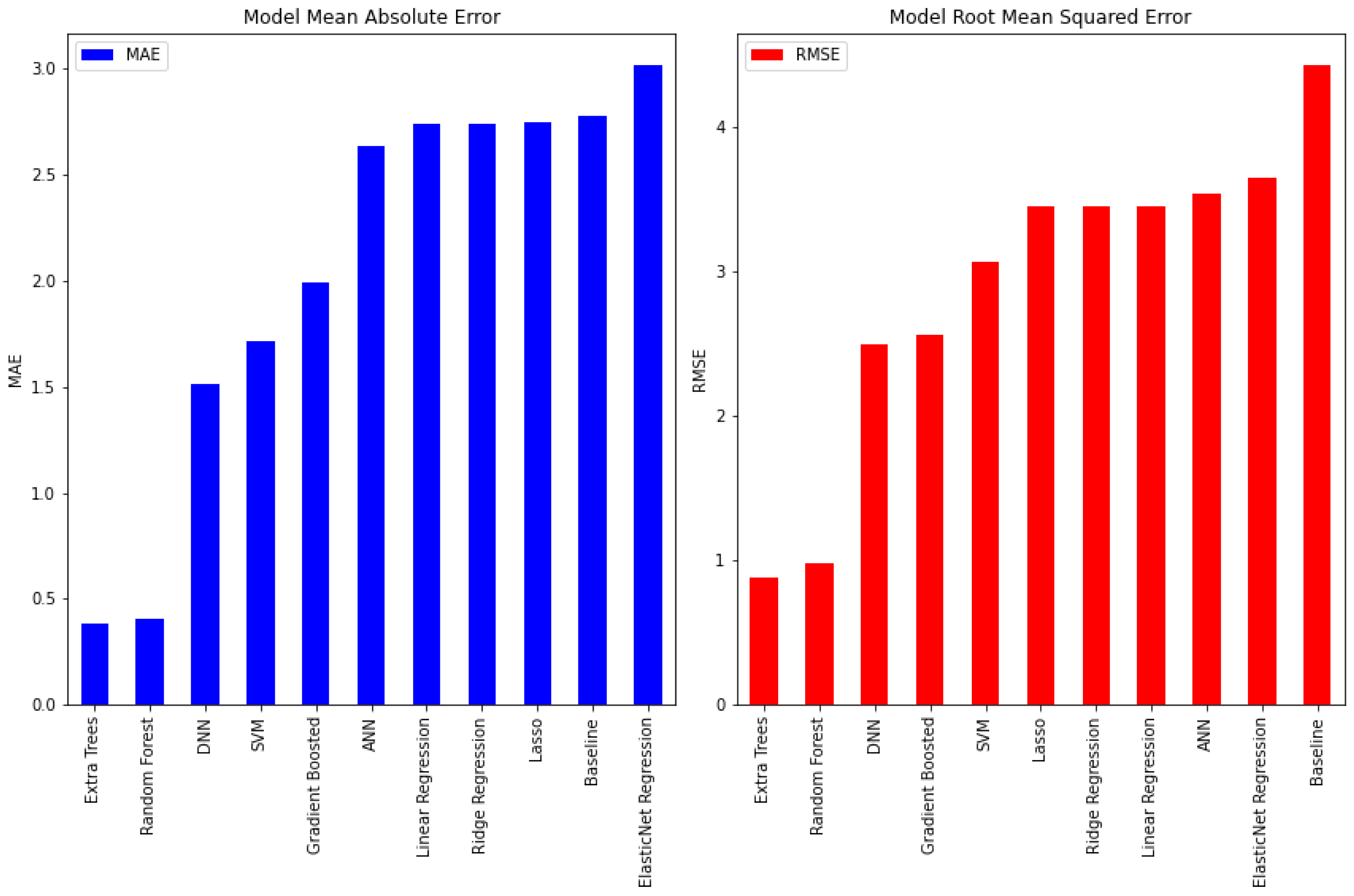
| Model | MAE | RMSE | Training Time (s) | Size (MB) |
|---|---|---|---|---|
| Baseline | 2.78 | 4.43 | 0.00 | 0.00 |
| Linear Regression | 2.74 | 3.45 | 0.00 | 0.0007 |
| Lasso | 2.75 | 3.45 | 0.08 | 0.005 |
| Ridge Regression | 2.74 | 3.45 | 0.00 | 0.0007 |
| ElasticNet Regression | 3.02 | 3.64 | 0.00 | 0.0007 |
| SVR | 1.72 | 3.06 | 0.21 | 0.321 |
| ANN | 2.64 | 3.54 | 8.29 | 0.061 |
| Gradient Boosting | 1.99 | 2.57 | 0.14 | 0.028 |
| DNN | 1.51 | 2.50 | 10.52 | 0.34 |
| Random Forest | 0.41 | 0.98 | 0.97 | 9.58 |
| Extra Trees | 0.39 | 0.88 | 16.41 | 30.4 |
| Model | MAE | RMSE | Training Time (s) | Size (MB) |
|---|---|---|---|---|
| Baseline | 2.91 | 4.64 | 0.00 | 0.00 |
| Linear Regression | 3.08 | 3.78 | 0.00 | 0.00 |
| Lasso | 3.41 | 4.04 | 0.11 | 0.01 |
| Ridge Regression | 3.08 | 3.78 | 0.01 | 0.00 |
| ElasticNet Regression | 3.10 | 3.79 | 0.01 | 0.00 |
| SVR | 2.81 | 4.50 | 0.27 | 0.23 |
| ANN | 3.08 | 3.78 | 15.11 | 0.06 |
| Gradient Boosting | 2.14 | 2.74 | 0.09 | 0.03 |
| DNN | 1.14 | 1.90 | 18.40 | 0.32 |
| Random Forest | 0.36 | 0.84 | 0.66 | 9.15 |
| Extra Trees | 0.27 | 0.72 | 9.38 | 28.94 |
| MAE (0.3/0.7) | RMSE (0.3/0.7) | Training Time (0.3/0.7) | Model Size (0.3/0.7) | |
|---|---|---|---|---|
| DNN | 2.41/3.12 | 3.29/4.39 | 6.17/4.8 | 0.31/0.31 |
| Random Forest | 0.58/0.7 | 0.90/1.2 | 0.09/0.06 | 0.84/0.36 |
| Extra Trees | 0.41/0.67 | 0.61/0.91 | 0.50/0.17 | 2.64/1.14 |
| Study | Problem | Features | Techniques | Dataset | Model Size | Training Time |
|---|---|---|---|---|---|---|
| [14] | Classification into three classes: rest before exercise, post-exercise, and after hydration | RR interval, RMSSD, and SDRR of ECG | SVM and K-means | 30 min ECG (10 min for each class) for 16 athletes (total = 480 min) | No | No |
| [7] | Classification into hydrated/mild dehydrated | 9 features from EDA and PPG | LDA, QDA, logistic regression, SVM, fine and medium Gaussian kernel, K-NN, decision trees, and ensemble of K-NNs | 8 min EDA and PPG for each of 17 subjects (total = 136 min) | No | No |
| [6] | Classification into hydrated/dehydrated | 9 statistical features from the GSR signal | Logistic regression, SVM, decision trees, K-NN, LDA, Naive Bayes | 2 h of EDA signal for each of 5 subjects (total = 600 min) | No | No |
| [4] | Classification into hydrated/dehydrated | Combinations of 6 statistical features extracted from the GSR signal | Logistic regression, random forest, K-NN, naive Bayes, decision trees, LDA, AdaBoost classifier, and QDA | EDA signals for 5 subjects, but they did not mention the recorded time | No | No |
| [15] | Classification into well-hydrated, hydrated, dehydrated, and very dehydrated | 12 features extracted from EDA and 2 features from the activity recognition model | Random forest, decision trees, naive Bayes, BayesNet, and multilayer perceptron | 24 h for 5 d of EDA signals, as well as activity labeling for 5 subjects (total = 36,000 min) | No | No |
| This study | Regression for the number of hours since last drinking | FEAT1(19) and FEAT2(12) as described in Section 4 | Linear, lasso, ridge, and ElasticNet regression, SVR, ANN, gradient boosting, DNN, random forest, and Extra Trees | Total of 3386 min for 11 subjects | Yes | Yes |
Publisher’s Note: MDPI stays neutral with regard to jurisdictional claims in published maps and institutional affiliations. |
© 2022 by the authors. Licensee MDPI, Basel, Switzerland. This article is an open access article distributed under the terms and conditions of the Creative Commons Attribution (CC BY) license (https://creativecommons.org/licenses/by/4.0/).
Share and Cite
Sabry, F.; Eltaras, T.; Labda, W.; Hamza, F.; Alzoubi, K.; Malluhi, Q. Towards On-Device Dehydration Monitoring Using Machine Learning from Wearable Device’s Data. Sensors 2022, 22, 1887. https://doi.org/10.3390/s22051887
Sabry F, Eltaras T, Labda W, Hamza F, Alzoubi K, Malluhi Q. Towards On-Device Dehydration Monitoring Using Machine Learning from Wearable Device’s Data. Sensors. 2022; 22(5):1887. https://doi.org/10.3390/s22051887
Chicago/Turabian StyleSabry, Farida, Tamer Eltaras, Wadha Labda, Fatima Hamza, Khawla Alzoubi, and Qutaibah Malluhi. 2022. "Towards On-Device Dehydration Monitoring Using Machine Learning from Wearable Device’s Data" Sensors 22, no. 5: 1887. https://doi.org/10.3390/s22051887
APA StyleSabry, F., Eltaras, T., Labda, W., Hamza, F., Alzoubi, K., & Malluhi, Q. (2022). Towards On-Device Dehydration Monitoring Using Machine Learning from Wearable Device’s Data. Sensors, 22(5), 1887. https://doi.org/10.3390/s22051887