Abstract
Activity recognition based on inertial sensors is an essential task in mobile and ubiquitous computing. To date, the best performing approaches in this task are based on deep learning models. Although the performance of the approaches has been increasingly improving, a number of issues still remain. Specifically, in this paper we focus on the issue of the dependence of today’s state-of-the-art approaches to complex ad hoc deep learning convolutional neural networks (CNNs), recurrent neural networks (RNNs), or a combination of both, which require specialized knowledge and considerable effort for their construction and optimal tuning. To address this issue, in this paper we propose an approach that automatically transforms the inertial sensors time-series data into images that represent in pixel form patterns found over time, allowing even a simple CNN to outperform complex ad hoc deep learning models that combine RNNs and CNNs for activity recognition. We conducted an extensive evaluation considering seven benchmark datasets that are among the most relevant in activity recognition. Our results demonstrate that our approach is able to outperform the state of the art in all cases, based on image representations that are generated through a process that is easy to implement, modify, and extend further, without the need of developing complex deep learning models.
1. Introduction
Ubiquitous computing has been envisioned as technology that provides support to everyday life, while disappearing into the background [1]. Disappearing into the background implies the goal of minimizing the technology’s intrusiveness and its demands of users [2]. A key aspect for supporting the everyday life of users is to be able to provide personalized services, for which is necessary to recognize what the user is doing. This task is known as Human Activity Recognition (HAR). The best performing approaches in that task to date are based on deep learning models. While the performance of the state-of-the-art approaches has been increasingly improving, a number of issues still remain. Specifically, we focus on the issue of the complexity of tuning or developing further the increasingly involved deep learning models considered for activity recognition, which incorporate ad hoc architectures of convolutional neural networks(CNNs), recurrent neural networks (RNNs), or a combination of both.
To cope with this issue in this paper we propose an approach that automatically transforms the inertial sensors time-series data into images that represent in pixel form patterns found over time, allowing even a simple CNN to outperform complex ad hoc deep learning models that combine RNNs and CNNs for activity recognition. Our approach can be considered as an extension of our preliminary workshop paper [3], where we introduce the concept of the image representation and present an initial evaluation with promising results. We have also presented in the past a similar approach but for the task of user identification [4]. In contrast to those two previous preliminary works, the current paper provides a clearer and more comprehensive rationale for the proposed image representations and details an image representation design and an image generation process that are more robust and capable of handling a wider range of scenarios. Furthermore, our evaluation in this case is much more extensive, comprising a wider range of experiments and configurations that allow to assess both the performance and the robustness of our proposed approach.
2. Related Work
2.1. CNNs for Time Series
In spite of the success that Convolutional Neural Networks (CNNs) have had in image processing tasks [5], due in part to their known capability of dealing with data with an intrinsic grid-like topology [6], a number of successful works have applied CNNs to time series data. In particular concerning ubiquitous computing, many works have proposed to use CNNs to deal with sensors time-series data (e.g., [7,8,9,10,11,12,13,14]). The majority of these previously proposed methods have been aimed at the task of activity recognition. In one of such works, a CNN is proposed to automate the feature learning from the raw sensor data in a systematic manner [9]. Another relevant related work uses a CNN combined with a long short-term memory (LSTM) network to extract time dependencies on features obtained by the CNN.
Similar to [7], the approaches in [12,13] combine CNNs with LSTMs. The approach in [13] uses a CNN to obtain high-level features, related to users’ behavior and physical characteristics. This is similar to the way the approach in [12] uses CNN for automated feature engineering. In [14], the authors use a distinct type of convolutional network, specifically a temporal convolutional network (TCN), which through a hierarchy of convolutions is able to entail the temporal relations of the time series data at different time scales.
The approaches mentioned above have used CNNs on time-series data in a direct way. That is, they have considered the time series as a one-dimensional grid, which is fed into the CNN directly. Instead, our approach creates 2D-image representations that entail patterns over time found in the time series. The resulting images are thus the input to a CNN model, with the intent of taking advantage of the strengths that CNNs have demonstrated when dealing with image processing tasks [5].
2.2. Image Representations of Time Series
A number of works have proposed to encode time series data into image representations, to then feed the images to a CNN to perform the classification (e.g., [15,16,17,18]). Specifically, in [15,16] the authors propose to encode time series using two different image representations: Gramian Angular Field (GAF) and the Markov Transition Field (MTF). The approach in [18] uses a similar encoding but for multiple time series. Other approaches have proposed to use a Short-time Fourier Transform (STFT) or Wavelet transform spectrogram to represent the time-series into image form (e.g., [19,20,21,22]).
Some approaches targeting HAR have proposed to form a 2D-image from the input signals (e.g., [23,24,25]). In these cases, the image formation consists simply in depicting the signals segments directly on an image. Therefore, it is as if the signals were imprinted on the images.
Approaches that simply depict the input signals directly on images (e.g., [23,24]) differ from our proposed method in that we first compute patterns over time from the time series data and then build an image that represents those patterns in a way that is better suited to be processed by a CNN, according to its widely recognized strengths, i.e., locality and edge detection [26]. On the other hand, approaches that have proposed an actual image representation, such as [15,18], use encodings that require relatively heavy computation, which make them unsuitable for real-time motion or action recognition [27]. In this respect, our approach is designed from the ground up to be easy to implement and represent a relatively low overhead.
3. Approach
Our approach is based on generating image representations from inertial sensors data. The generated images are then used as the input instances for a convolutional neural network (CNN) for activity recognition. Specifically, our image generation process is designed as to produce images that (a) take advantage of 2 well known strengths of CNNs, namely locality and edge detection [26], and (b) depict as many relevant patterns over time as possible in a single image.
3.1. Image Generation Process
To simplify the explanation, we first start with the case of one time window from an univariate time series and a single pattern. From the univariate time series, we take a time window , from which we compute a pattern over time (see Section 3.2). We then transform the value of the pattern into pixel form (see Section 3.5), placing this on a specific region of the image (see Section 3.3). This process is illustrated in Figure 1. For a multivariate time series, each component of the time series is taken separately and represented in a different region of the image. The same is the case for neighboring time windows, i.e., each time window is represented in a specific region of the image. Following this process, it is possible to represent in a single-channel image as many patterns, time series components, and neighboring windows as needed by incorporating more regions of the image. Furthermore, color images (with 3 channels, i.e., RGB) allow to represent even more information on the regions that compose the extra channels (see Section 3.7). The time windows we consider are non-overlapping, as we found this to be the best configuration, since considering overlapping windows just slowed down the process without any evident improvement in performance.
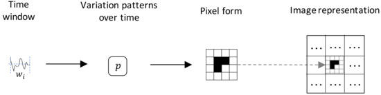
Figure 1.
Image generation process.
3.2. Patterns over Time
We consider patterns that emerge over time in a single time window of an univariate time series. We decided for a set of patterns that are simple to compute and that can help effectively distinguish between different activities. Other methods in the literature have considered to either depict directly part of the signal on the image or depict the result of signal transformations such as Fourier Transform (e.g., [19]) or Wavelet Transform (e.g., [20,21,22]). In the first case, the design effort is placed on the neural network architecture, which is something we are seeking to avoid with our approach. Concerning the second case, the transformations used involve heavy computation [27], which stands in contrast to the simple computations needed in our case.
Specifically, the patterns we consider are:
- Oscillatory variation. This pattern refers to the case in which the value of the data points in the time window go up and down from one time step to the next one. Specifically, if we consider 3 consecutive time steps , , and , where , we have either that at times and the values of the corresponding data points and are strictly higher than the value of the data point at time , or that at time the value of the corresponding data point is strictly higher than both the values of the data points at and at . This pattern is illustrated on the blue areas shown in Figure 2.
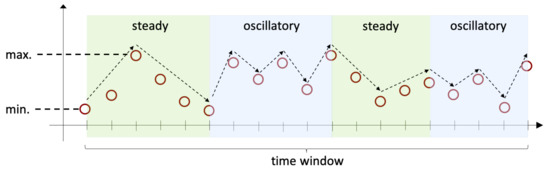 Figure 2. Variation patterns over time.
 - Steady variation. This pattern refers to the case where the value of the time window goes either up or down consistently. This is illustrated on the green areas in Figure 2.
- Range. This pattern refers to the maximum, minimum, and the difference between maximum and minimum data point values within the time window.
As we can observe in Figure 2, within one time window it is possible to recognize more than one type of variation patterns. To compute the value of either variation pattern (), we consider all segments within the time window where the data points of the respective pattern are present and we use the formula in Equation (1), where corresponds to the value of the data point at time step and to the value of the data point at the previous time step, i.e., . Note that since in order to recognize the type of variation pattern we need at least 3 data points, it is ensured that in the equation.
3.3. Canvas & Regions [Locality]
In order to obtain images that purposely exploit the locality strength of CNNs, we seek to consistently represent specific pattern(s) in specific regions of the images. To this end, we consider an image as an empty ‘canvas’ or number of regions and C number of channels. Black and white (B & W) images correspond to , while color (RGB) images to . Each region is composed of number of pixels. A canvas divided into regions as explained is illustrated in Figure 3.
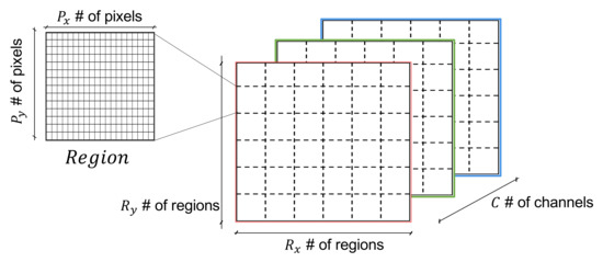
Figure 3.
Canvas & Regions [locality].
In this paper, we consider the following specific design for the images. The canvas is split into 36 regions () and these cover a total of 4 quadrants, which correspond to 9 regions (). This canvas is depicted in Figure 4, where it can be seen that the oscillatory and steady variations are placed on the top-left and top-right quadrants, respectively. On the other hand, range patterns are placed at the bottom, namely the maximum is on the bottom left and the difference between maximum and minimum is on the bottom right.
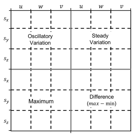
Figure 4.
Canvas, quadrants, regions.
We further enrich the image representations by including patterns found in neighboring time windows. In particular, as depicted in Figure 4, each region represents a pattern corresponding to one of the components of the inertial sensor (, , and ) for a specific window span (u, w, or v). In this case w corresponds to the current time window, u to the windows before the current window, and v to the windows after the current window. In this paper, we consider two windows for u and v, namely the regions covered by u correspond to patterns found in the two windows before the current one, and the regions covered by v refer to patterns found in the 2 windows after the current window.
3.4. Pixel Filling [Edge Detection]
To generate images that can exploit the edge detection strength of CNNs, we seek to produce clearly distinguishable edges that represent the patterns of interest in a consistent manner. To this end, we introduce the concepts of ‘marked’/‘unmarked’ pixels and of ‘continuous pixel marking’. A ‘marked’ pixel corresponds to the value 255 (i.e., white color), whereas an ‘unmarked’ pixel corresponds to the value 0 (i.e., black color). We have chosen the such contrast between ‘marked’ and ‘unmarked’ pixel to accentuate the edges produced. Continuous pixel marking refers to filling in the pixels in a region by marking them consecutively based on a specific ‘filling’ strategy (see Section 3.6). This is illustrated in Figure 5. As we can see in the figure, by using continuous pixel marking we ensure the generation of well-defined and continuous edges.
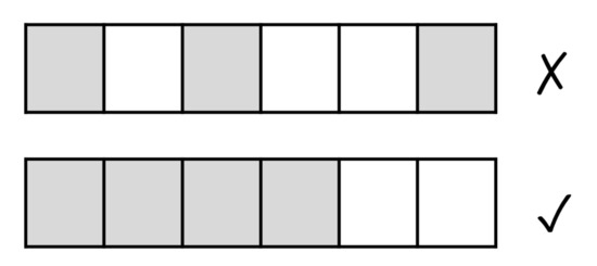
Figure 5.
Continuous pixel marking (on the bottom) [edge detection].
3.5. Mapping Inertial Sensors to Pixels
To obtain the number of ‘marked’ pixels corresponding to a given pattern value, we define a mapping function M as:
To compute this we need to consider the minimum () and maximum () values of the given pattern for the current time window, and the minimum () and maximum () number of pixels that can potentially be ‘marked’ within a region. This allows to transform any given pattern value into the corresponding number of ‘marked’ pixels within a region, according to Equation (3).
As it can be observed in Equation (3), the value of is ensured to be a whole number, since we are considering the floor function. In this way, the value is easily translatable into the number of ‘marked’ pixels. Any pixel that is no ‘marked’ is considered ‘unmarked’.
3.6. Filling Strategies
A number of different fillings strategies can be proposed. For this paper, we only focused on strategies aimed at producing images with well localized and distinguishable edges that can be easily reproduced. Next, we describe the filling strategies we consider, which are illustrated in Figure 6.
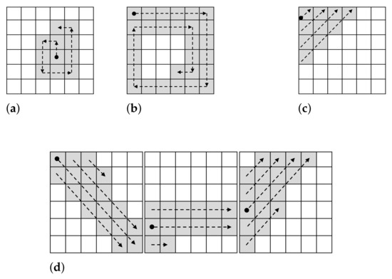
Figure 6.
Filling strategies. (a) Counterclockwise (CCW); (b) Clockwise (CW); (c) Diagonal (Diag); (d) Strokes (Strk).
- Counterclockwise (CCW). This strategy, which is illustrated in Figure 6a, starts at the center pixel of the region, or in the pixel right before the center in the case of a region with an even number of pixels. From that point, the ‘marked’ pixels are filled in continuously, first up one pixel, then left, then down, and so on in a counterclockwise manner. The path that it is followed is such that does not considers the same pixel twice and leaves no pixel ‘unmarked’ on the way.
- Clockwise (CW). This strategy (illustrated in Figure 6b) starts at the pixel of the top-left corner of the region. The path then makes pixels ‘marked’ in a clockwise fashion, while avoids considering the same pixel twice or skipping any pixel.
- Diagonal (Diag). This strategy that is depicted in Figure 6c has the pixel at the top-left corner of the region its starting point. The path from there corresponds to a 45° diagonal that goes upwards. The pixels are never considered twice and the pixels on the path are never left ‘unmarked’.
- Strokes (Strk). This strategy (see Figure 6d) seeks to produce continuous ‘strokes’ that pass over 3 regions of the same row of the image representation. To do this, we consider for each of the regions on the row diagonal or horizontal lines, which are then followed on the next region by a different type of line. That is, the path considered in the first region on the left is of reverse diagonals. This is then followed in the next region by a path of horizontal lines. Finally, the last region considers a path of diagonal lines. The lines are drawn from left to right and are stacked one on top and one on the bottom of the latest line. By default we consider the top-left corner the beginning of the path. This is true for the first left-most region and for any region where no pixel has been marked in the previous region to the left that is directly adjacent to the region under consideration. If the case is different, then the starting point considered is the one next to the highest ‘marked’ pixel in the previous region to the left which is directly adjacent to the region under consideration. In Figure 6d an example of this strategy is shown. As it can be seen, the left-most region starts at the top-left corner (depicted by a black dot) and it goes into filling that reverse diagonal, then the one on the top of that, then the one on the bottom of the first one, and finishes half-way through the diagonal on top of the second diagonal. The next region to the right then starts at the pixel that is adjacent to the highest ‘marked’ pixel in the previous region, using horizontal lines from left to right, and filling next the line on top of the first one and then the line below. The third region is filled in a similar way, but following diagonal lines.
3.7. Coloring
In order to incorporate further information as part of the image representations we consider the three channels of a color (RGB) image, namely red, green, and blue. In this paper, we propose two ways of using the color channels. One option is to represent patterns found in time windows next to the current time window. The second option we propose is to depict patterns from multiple sensors, using each color channel to represent the patterns of a different sensor.
3.7.1. Color Channels to Represent Nearby Time Windows
For this option we propose two different alternatives. The first one, depicted in Figure 7, is a simple assignment of the current window w, the window(s) u before the current one, and the window(s) v following the current one to each of the color channels.
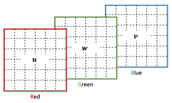
Figure 7.
Simple color channel assignment to represent nearby time windows patterns.
The second option we propose to represent neighboring time windows patterns is aimed at representing in a different manner the window , which is right before the current window than the window , which precedes , and similarly for the windows after the current one. Specifically, for this case all channels use the same canvas with the same ‘marked’ and ‘unmarked’ pixels, obtained as we explained previously. However, the specific pixel value of each of the ‘marked’ and ‘unmarked’ pixels is based on the previous windows (i.e., and ) for the red channel, on the current window for the green channel, and on the following windows (i.e., and ) for the blue channel. The purpose of this is to encode in the color of the image as much information as possible of what can be found in the neighbor time windows of the current one. The red channel’s ‘marked’ pixels are derived from considering the value of the pattern corresponding to the same area for the image representing one window before the previous (i.e., ) scaled within the range of color values . This is . After that, the pixel value is obtained by adding to the minimum possible pixel value (i.e., 0) as . The process for the red channel’s ‘unmarked’ pixels, on the other hand, considers the pattern corresponding to the immediate previous window (i.e., ), which is scaled within the range of possible pixel values to obtain . Then, the pixel value is obtained by subtracting from the maximum possible pixel value (i.e., 255) as . The pixel value for the green channel is obtained considering the scaled pattern value of the current window as for ‘marked’ pixels and for ‘unmarked’ pixels. Finally, the pixel values for the blue channel’s ‘marked’ and ‘unmarked’ pixels are obtained as and , respectively. This process is illustrated in Figure 8, focusing only on one specific region in the middle of a particular quadrant within an image representation. As it can be observed, all the channels in the color image at the bottom of the figure share the same ‘marked’ and ‘unmarked’ pixels, which follows the configuration found in the image representing . The difference is only on the pixel value that each of the ‘marked’ and ‘unmarked’ pixels will have on each of the channels.
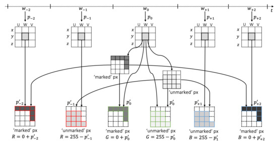
Figure 8.
‘marked’ and ‘unmarked’ coloring based on nearby windows.
3.7.2. Color Channels to Represent Multiple Sensors
In this option, the patterns of each inertial sensor is represented on a different color channel, as illustrated in Figure 9. This can be a good option when dealing with inertial measurement units (IMUs), which typically contain an accelerometer, a gyroscope, and a magnetometer. However, it has the clear limitation imposed by the number of available color channels, which makes it unsuitable when considering more than 3 inertial sensors. For such a case, we propose below the augmentation of the canvas.
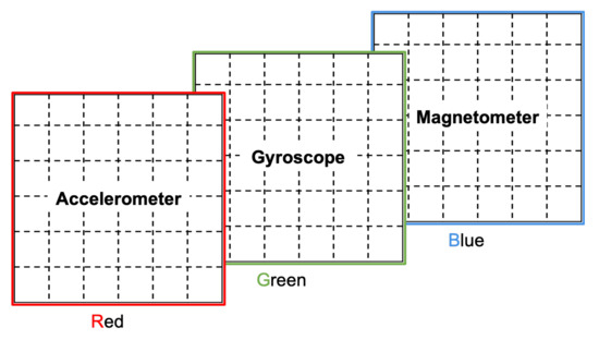
Figure 9.
Simple color channel assignment to represent multiple sensors.
3.8. Augmented Canvas for Multiple Sensors
To incorporate patterns from more than one sensor, we consider images of larger size, which are obtained by placing side by side images generated from different sensors. This is illustrated in Figure 10, where we see a sample of an image generated with our approach for different the USC-HAD dataset.
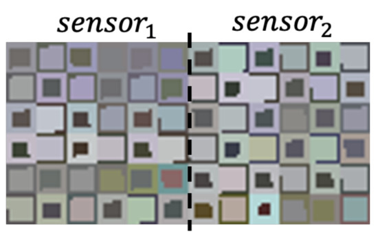
Figure 10.
Augmented canvas for multiple sensors.
4. Evaluation Methodology
To evaluate our approach, we consider 7 of the most widely recognized datasets in HAR [28], comparing for each dataset the performance of our method against the methods in the literature that we found have achieved highest performance. We provide the comparison with respect to at most 5 other approaches with best performance in the literature for each dataset. Specifically, the datasets we consider are WISDM, UCI-HAR, USC-HAD, PAMAP2, Opportunity, Daphnet, and Skoda. In each case, we configure our image representations to make use of the same inertial sensors considered by the state-of-the-art approaches and measure the performance using the same metrics they use. Concerning the machine learning evaluation, to ensure that the comparison is fair, we consider the same metric as the one used in the paper where the approach was proposed and evaluated. Furthermore, the data split we use on each case corresponds to the one considered by what we found to be the best performing approach for the corresponding dataset. As a baseline we consider a simple convolutional neural network (CNN) defined as follows. Two convolutional layers, each considering 128 filters of size 3 × 3. Each convolutional layer is followed by a max-pooling layer, with filter size of 2 × 2 and a stride of 2. These layers are followed by a dense layer of 256 units. Furthermore, we use softmax activation on the last layer, ReLU on the intermediate layers, cross-entropy loss function, Adam optimizer, and early stopping. For the image generation process, we consider in all cases CCW and CW filling strategies for each region in an iterative sequence (i.e., CCW, CW, CCW, …). The coloring strategy we used is the one illustrated in Figure 8. We decided to use this design as we found it to be the best one in terms of the results yielded. The implementation was made using the Keras library, https://keras.io/ (accessed on 27 December 2021).
4.1. Datasets
4.1.1. WISDM Dataset
This dataset https://www.cis.fordham.edu/wisdm/dataset.php (accessed on 27 December 2021) was collected from a smartphone, only considered the accelerometer. In [29], was the first time that the dataset was introduced and detailed. A total of 36 users were considered for the collection, where each user followed 6 activities: going up and down the stairs, jogging and walking, as well as standing. Figure 11a depicts a sample of an image representation that our approach generated for this dataset. For the machine learning evaluation we consider a 10-fold cross-validation, as described in what we found to be the best performing approach in the literature for this dataset, namely Hossain et al. [30].
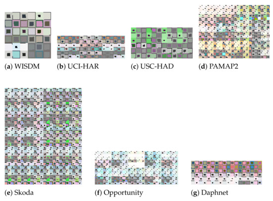
Figure 11.
Samples of the image representations: (a) WISDM (120 × 120 px.), (b) UCI-HAR (180 × 60 px.), (c) USC-HAD (120 × 60 px.), (d) PAMAP2 (120 × 90 px.), (e) Skoda (120 × 150 px.), (f) Opportunity (150 × 60 px.), and (g) Daphnet (180 × 60 px.)
4.1.2. UCI-HAR Dataset
This dataset https://archive.ics.uci.edu/ml/datasets/human+activity+recognition+using+smartphones (accessed on 27 December 2021) was also collected data using a smartphone. In this case the smartphone was waist-mounted and the data recorded corresponds to the accelerometer and the gyroscope in the smartphone. In [31], the authors introduced first this dataset, which collected data from 30 users. The image generation considered in this case took the time series corresponding to acceleration from the accelerometer, estimated body acceleration, and angular velocity from the gyroscope. As mentioned in Section 3.8, when considering multiple inertial sensors, we put together in a single image each of the images generated from every single sensor’s data. Figure 11b shows a sample of an image representation that was generated by our approach from this dataset. For the machine learning evaluation, we consider 10-fold cross validation, as it was considered by what we found to be the best performing approach in the literature for this dataset, i.e., Ignatov [24].
4.1.3. USC-HAD Dataset
This dataset http://sipi.usc.edu/had/ (accessed on 27 December 2021) considers 12 simple activities, such as walking, running, jumping, sitting, standing, and sleeping. The number of participants for the data collection was 14. The inertial sensors used were accelerometer and gyroscope, which are the ones used for the image generation in our case. A sample of the image representations generated for this dataset can be seen in Figure 11c. The machine learning evaluation in this case is made considering a random 80% (training), 20% (testing) split, as described in what we found to be the best performing approach for this dataset, namely Murad and Pyun [32].
4.1.4. PAMAP2 Dataset
This dataset http://www.pamap.org/demo.html (accessed on 27 December 2021) considers 3 IMUs places on the chest, arm and ankle of a total of 9 participants. The activities performed were 18. The generated images for this dataset place side by side 12 images, each of which was generated for each IMU. In Figure 11d, we can observe a sample of an image representation generated from this dataset. For the machine learning evaluation we consider a random 80% (training), 10% (validation), and 10% (testing) split, as described in what we found to be the best performing approach for this dataset, namely Jafari et al. [25].
4.1.5. Opportunity Dataset
We consider the Opportunity ‘challenge’ dataset http://www.opportunity-project.eu/challengeDataset.html (accessed on 27 December 2021) first used in [33]. The data considers 4 participants performing 6 different iterations of broad morning routines and a set of specific activities such as opening and closing the fridge, opening and closing the dishwasher, turn on and off the lights, drinking, and cleaning the table. The dataset was recorded with each participant wearing 12 accelerometers in different parts of their body. The image representations for this dataset are obtained by placing side by side the images generated from 10 of the sensors. The reason to consider only 10 out of the 12 accelerometers is to have a similar configuration with respect to the state-of-the-art approaches against which we compare the performance of our approach. A sample of a generated image for this dataset is shown in Figure 11f. The machine learning evaluation in this case was performed using a 10-fold cross-validation, as described in what we found to be the best performing approach in the literature for this dataset, namely Hossain et al. [30].
4.1.6. Daphnet Freezing of Gait Dataset
This dataset https://archive.ics.uci.edu/ml/datasets/Daphnet+Freezing+of+Gait (accessed on 27 December 2021) considers 10 subjects wearing 3 accelerometers. The goal is to detect sudden and transient inability to move, known as Freeze of Gait, while the participants walk [34]. The image representations in this case are generated by concatenating three image representations, one for each of the three accelerometers. A sample of an image representation for this dataset is depicted in Figure 11g. The split used for the machine learning evaluation in this case was 10-fold cross-validation, as described by what we found to be the best performing approach for this dataset, i.e., Hossain et al. [30].
4.1.7. Skoda Mini Checkpoint Dataset
This dataset http://har-dataset.org/lib/exe/fetch.php?media=wiki:dataset:skodaminicp:skodaminicp_2015_08.zip (accessed on 27 December 2021) was collected from 8 subjects performing 10 times a car checking procedure. Each participant performed the tasks while wearing a special motion jacket with 7 IMUs. The dataset was first introduced and used in [35]. Our image representations in this case are generated based on data 16 inertial sensors, in order to have a fair comparison to the approaches against which we compare our approach’s performance. A sample of an image representation for this dataset is depicted in Figure 11e. For the machine learning evaluation we consider a random 80% (training), 10% (validation), and 10% (testing) split, as described in what we found to be the second-best performing approach for this dataset in the literature, namely Zeng et al. [36]. We consider the second-best because the best performing approach in this case, did not mention the split used.
4.2. Metrics
We consider standard metrics used to measure the performance of machine learning classification approaches, according to what the state-of-the-art methods in our benchmark have used. In a basic binary classification one may have the following basic options: (a) true positives (TP) when the model correctly predicts the positive class, (b) false positives (FP) when the model mistakenly predicts the positive class, (c) false negatives (FN) when the model wrongly predicts the negative class, and (d) true negative (TN) when the model correctly predicts the negative class. Based on this, we define the metrics (Equation (4)), (Equation (5)), (Equation (6)) and -score (Equation (7)) used in our evaluation in a per-class basis.
5. Results
5.1. Benchmarking
In this section, we conduct a comparison of the performance of our approach against the best performing approaches we were able to find in the literature. We first focus on other approaches that also proposed image representations for HAR. Then, we compare the performance of our approach against the results reported in the papers that have introduced the best performing approaches that we could find in the literature, for each of the datasets we consider.
5.1.1. Comparison to Existent Image Representations
We were able to find three existing approaches in the literature that have proposed image representations for HAR (i.e., [23,24,25]). Table 1 shows a comparison between the performance of our approach and each of these three existing approaches. The comparison is made considering the same datasets used in the papers where each of these related works were introduced. Furthermore, we consider the same metric as the one considered in each respective paper, seeking to obtain a fair comparison. Likewise, the data split we use for machine learning evaluation on each case, corresponds to the one considered by what we found to be the best performing approach for the corresponding dataset. The results of these works are taken directly as presented by their authors.

Table 1.
Performance: our approach vs. other existent image representation approaches for Activity Recognition.
As we can see in Table 1, in terms of performance, our approach is able to outperform these existing methods in all the cases considered. Furthermore, our approach is only concerned with the construction of image representations, which does not require any specialized deep learning expertise or involvement for implementation or further development, whereas the other methods propose both an image representation and a specific CNN architecture (e.g., Sensornet architecture [25]).
5.1.2. Comparison to Best Performing Approaches for Each Dataset
In this section, we present the comparison between the performance of our approach and the best performing approaches in the literature, for each of the 7 datasets that we consider. The performance result from the state-of-the-art approaches is reported exactly as it appears on the paper where the approach was first introduced.
WISDM Dataset
The results of the evaluation of our approach using this dataset are presented in Table 2. As we can see, our approach shows a higher accuracy with respect to all state-of-the-art approaches. In all cases, the approaches under consideration use neural networks, particularly CNNs. In particular, in [24] time series data is treated as image data and passed through a CNN, in [37,38] the authors propose a new CNN architecture to deal with HAR, and in [19] the authors combine deep learning models with spectrograms and Hidden Markov Models (HMM) to perform the activity recognition. Among the approaches considered, it is worth noting that our approach is able to outperform the approach in [30], which it is an approach that uses user input through active learning to improve the accuracy.
Table 2.
Comparison considering WISDM dataset.
UCI-HAR Dataset
The results of the evaluation of our approach using this dataset are presented in Table 3. Our approach clearly outperforms the state of the art when considering this dataset. The state-of-the-art approaches include in this case an end-to-end deep learning model [40], a method that stacks the raw signals from the inertial sensors into images which serve as the input instances to a CNN [23], a method that treats time series data as image data [24], and an approach that uses directly the time series as the input of the CNN [41].
Table 3.
Comparison considering UCI-HAR dataset.
USC-HAD Dataset
The comparison of our results against the results of the state of the art for this dataset are presented in Table 4. As we can see, the performance of our approach is higher that the one of the existing methods. Interestingly, for this dataset we get to compare our approach to two methods that consider Long short-term memory (LSTM) models (i.e., [32,42], which are recurrent neural networks that have been proposed particularly to deal with time series data. In any case, our approach manages to outperform all existing methods in the state of the art.
Table 4.
Comparison considering USC-HAD dataset.
PAMAP2 Dataset
The comparison of our results against the results of the state of the art for this dataset are presented in Table 5, where we can see that our approach has a higher performance overall. The state of the art in this case includes an approach that consider LSTM models [36], two approaches that propose the use of a combination of a CNN and a recurrent model to account for both spatial and temporal patterns (i.e., [10,43]), and an approach that transforms multimodal time series into images that are then used as input to a CNN [25]. Although this approach also considers image representations of time series, our results show that our encoding achieves a better accuracy.
Table 5.
Comparison considering PAMAP2 dataset.
Opportunity Dataset
The comparison of our results against the results of the state of the art for this dataset are presented in Table 6. As it can be observed, our approach outperforms the state of the art, which includes approaches that consider LSTM models alone [10] and in combination to CNNs [7,44], as well as an approach that considers the active input from users to improve the performance [30].
Table 6.
Comparison considering Opportunity dataset.
Daphnet Freezing of Gait Dataset
The comparison of our results against the results of the state-of-the-art approaches for this dataset are presented in Table 7. Our approach is able to outperform the best performing exiting approaches for this dataset, including an approach that considers data from multiple sensors and the machine learning concept of attention to improve performance [45], an end-to-end deep learning approach [40], and an approach to deal with HAR based on active learning [30].
Table 7.
Comparison considering Daphnet dataset.
Skoda Mini Checkpoint Dataset
The comparison of our results against the results of the state-of-the-art approaches for this dataset are presented in Table 8. The approaches in the literature with highest performance for this dataset include an ensemble method that obtains its results best on the best results from a set of LSTM models [46], approaches that consider the machine learning concept of attention to improve performance [36,47], and an end-to-end approach that combines convolutional networks and LSTM models to account for the spatio-temporal patterns in the data [7]. In all cases, our approach is able to outperform their performance.
Table 8.
Comparison considering Skoda Mini checkpoint dataset.
5.1.3. Summary of Benchmarking
In Table 9, we summarize the overall results of our evaluation, where we present the performance of our approach against the results of the best performing approach in the literature for each of the 7 datasets we consider.
Table 9.
Our approach vs. best approaches in the literature.
We can make two main observations about the results in Table 9 and in general of the comparison we have made with respect to all state-of-the-art approaches in the literature. The first one is that our approach is able to outperform each of the best performing approaches for all the datasets we consider. While the difference between our results and the existent approaches is not substantial (avg. = 0.0278), it provides evidence that overall our approach is sound and capable of handling a wide variety of datasets, maintaining a top performance. The second observation is that compared to our approach, all the state-of-the-art approaches are making use in general more sophisticated machine learning methods or consider more complex or elaborate neural network architectures. One approach considers active learning during the fine tuning phase in order to single out the most informative data instances [30]. Two other approaches proposed the use of neural network architectures based on U-Net [39], which contain large amounts of layers (23 conv. layers [38] and 28 conv. layers [48]). With the goal of accounting for temporal information, 5 approaches propose the use of LSTMs, either alone [10,32,42] or in combination with CNNs [7,43,44]. All this stands in contrast to our approach, where the CNN architecture is not at all the main focus and it is rather basic (i.e., 2 conv. layers followed each by a pool layer). Instead, our approach focuses on the design of the image representation, which does not require any specialized deep learning expertise for its use or further extension.
5.2. Comparison between Different Canvas Layouts
In order to account for the robustness of our approach, in this section we present the performance of our approach when modifying the baseline layout of the canvas that we used during all other experiments. This baseline layout is the one introduced in Section 3 and illustrated in Figure 4. The modifications are simple switching of halves or quadrants as specified in Table 10. The goal is to identify if the specific layout proposed as baseline is in fact relevant or if the regions can be moved around as long as the design is maintained consistent throughout the generation of the image representations. This experiment was conducted only for the WISDM dataset, since it is the simplest dataset in terms of the number of time series variables involved, which allows us to focus only on analyzing if the performance of the approach is greatly affected by the layout or not.
Table 10.
Comparison between different canvas layouts.
As we can see from the results in Table 10, the performance of our approach does not show much difference regardless of the specific layout used. Even for the case in which the quadrants are flattened over the rows of the canvas, and so the layout of the regions is modified almost completely, the performance of the approach remains very similar with respect to the case when the baseline layout is considered, with only a −0.0093 difference.
6. Discussion
6.1. Threats to Validity
The main threat to validity to our evaluation is that although we have used what we found to be the most widely recognized and used datasets in activity recognition from inertial sensors, the number of different activities considered is very constrained. This is because these datasets mostly consider very simple activities, such as walking and jogging, and overall they focus in the same activities or very similar ones, such as going up and down the stairs. Among the datasets, perhaps the one with activities that are different with respect to the ones in the other datasets is Skoda. However, on the downside it focuses on very specialized activities that might not correspond to activities performed by most users in real life scenarios. An inevitable workaround for this issue would be to collect a brand new dataset that includes a wider variety of scenarios and activities as well as a larger set of users.
6.2. Approach Limitations
An important limitation of our approach is that it requires some manual work related to the definition of the overall design used for the automatic generation of image representations. However, we have seen that, on the one hand, the manual work required for the configuration of such design is not heavier than the one required to configure a deep learning model, for which in addition specialized knowledge is needed. On the other hand, as we have observed in our experiments of Section 5.2, our approach is in general robust to changes in the configuration used in the design of the image representations. Therefore, we believe the manual work involved in our approach is considerably lower than its positives, particularly when compared to the work required in configuring complex ad hoc deep learning models.
6.3. Approach Practicality
In this section, we analyze the practicality of our approach, namely the challenges that one may encounter when taking it into a real-world application. In this respect, we believe that the biggest concern may be the impact on performance, specifically related to the efficiency with which a given activity can be recognized. In spite of this, we believe that our approach does not imply a big overhead. On the one hand, it is not hard to see that the algorithmic complexity of our image generation process is , as the only operation involved is a sum of differences to compute the variation patterns over the time series. On the other hand, throughout our experiments, we found that the average time to generate an image representation is 0.044 seconds using a non-specialized GPU (we use Google Colaboratory’s basic GPU for all our computations), which we believe does not correspond to a major overhead when compared to the duration of the activities considered.
Another issue that may affect performance refers to the bottleneck caused by the use of nearby time windows to generate the image representations. We believe, however, that this could be alleviated by disregarding information from windows after the current window, in place of a model that improves continuously over time.
7. Conclusions
The recent success of deep learning in human activity recognition from inertial sensors has brought about many new approaches that have focused on improving the performance based mainly on proposing different architectures. In spite of this success, a relevant issue is related to how challenging may be to tune or developing further the increasingly involved deep learning models considered for activity recognition, which include ad hoc CNN and RNN architectures. In this paper, we have proposed an approach that automatically transforms inertial sensors time-series data into images that represent in pixel form patterns found over time, allowing even a simple CNN to outperform complex ad hoc deep learning models for activity recognition. We have evaluated our approach against the best performing approaches in the literature for 7 of the most widely known datasets in HAR. Our evaluation shows that our approach is able to achieve higher performance that the state of the art in all of these datasets and exhibits robustness across different configurations The main limitation of our approach is related to the work required to define the image representation designs. In spite of this, we have aimed at providing simple designs that are easy to implement and develop further.
Author Contributions
Software, M.S.; Supervision, M.M.; Research, Writing—original draft, A.S.G. The authors contributed equally in all parts of the article in terms of literature review, adopted methodology, feature identification, model definition, experimentation and results analysis. All authors have read and agreed to the published version of the manuscript.
Funding
This work has been funded by the LOEWE initiative (Hesse, Germany) within the emergenCITY centre. We acknowledge support by the Deutsche Forschungsgemeinschaft (DFG—German Research Foundation) and the Open Access Publishing Fund of Technical University of Darmstadt.
Institutional Review Board Statement
Not applicable.
Informed Consent Statement
Not applicable.
Conflicts of Interest
The authors declare no conflict of interest.
References
- Weiser, M. The Computer for the 21 st Century. Sci. Am. 1991, 265, 94–105. [Google Scholar] [CrossRef]
- Myles, G.; Friday, A.; Davies, N. Preserving privacy in environments with location-based applications. IEEE Pervasive Comput. 2003, 2, 56–64. [Google Scholar] [CrossRef] [Green Version]
- Guinea, A.S.; Sarabchian, M.; Mühlhäuser, M. Image-based Activity Recognition from IMU Data. In Proceedings of the 2021 IEEE international conference on pervasive computing and communications workshops (PerCom workshops), Kassel, Germany, 22–26 March 2021. [Google Scholar]
- Sanchez Guinea, A.; Heinrich, S.; Mühlhäuser, M. VIDENS: Vision-based User Identification from Inertial Sensors. In Proceedings of the 2021 International Symposium on Wearable Computers, Virtual Event, 21–26 September 2021; pp. 153–155. [Google Scholar]
- Khan, A.; Sohail, A.; Zahoora, U.; Qureshi, A.S. A survey of the recent architectures of deep convolutional neural networks. Artif. Intell. Rev. 2020, 53, 5455–5516. [Google Scholar] [CrossRef] [Green Version]
- Goodfellow, I.; Bengio, Y.; Courville, A. Deep Learning; MIT Press: Cambridge, MA, USA, 2016. [Google Scholar]
- Ordóñez, F.J.; Roggen, D. Deep convolutional and lstm recurrent neural networks for multimodal wearable activity recognition. Sensors 2016, 16, 115. [Google Scholar] [CrossRef] [Green Version]
- Ha, S.; Yun, J.M.; Choi, S. Multi-modal convolutional neural networks for activity recognition. In Proceedings of the 2015 IEEE International conference on systems, man, and cybernetics, Hong Kong, China, 9–12 October 2015; pp. 3017–3022. [Google Scholar]
- Yang, J.B.; Nguyen, M.N.; San, P.P.; Li, X.L.; Krishnaswamy, S. Deep convolutional neural networks on multichannel time series for human activity recognition. In Proceedings of the 24th International Conference on Artificial Intelligence, Buenos Aires, Argentina, 25–31 July 2015; pp. 3995–4001. [Google Scholar]
- Hammerla, N.Y.; Halloran, S.; Plötz, T. Deep, convolutional, and recurrent models for human activity recognition using wearables. In Proceedings of the Twenty-Fifth International Joint Conference on Artificial Intelligence, New York, NY, USA, 9–15 July 2016; AAAI Press: Palo Alto, CA, USA, 2016; pp. 1533–1540. [Google Scholar]
- Ha, S.; Choi, S. Convolutional neural networks for human activity recognition using multiple accelerometer and gyroscope sensors. In Proceedings of the 2016 International Joint Conference on Neural Networks (IJCNN), Vancouver, BC, Canada, 24–29 July 2016; pp. 381–388. [Google Scholar]
- Chen, L.; Zhang, Y.; Peng, L. METIER: A Deep Multi-Task Learning Based Activity and User Recognition Model Using Wearable Sensors. Proc. ACM Interact. Mob. Wearable Ubiquitous Technol. 2020, 4, 5. [Google Scholar] [CrossRef] [Green Version]
- Huang, A.; Wang, D.; Zhao, R.; Zhang, Q. Au-Id: Automatic User Identification and Authentication Through the Motions Captured from Sequential Human Activities Using RFID. Proc. ACM Interact. Mob. Wearable Ubiquitous Technol. 2019, 3, 1–26. [Google Scholar] [CrossRef]
- Sheng, T.; Huber, M. Weakly Supervised Multi-Task Representation Learning for Human Activity Analysis Using Wearables. Proc. ACM Interact. Mob. Wearable Ubiquitous Technol. 2020, 4, 57. [Google Scholar] [CrossRef]
- Wang, Z.; Oates, T. Encoding time series as images for visual inspection and classification using tiled convolutional neural networks. In Proceedings of the Workshops at the Twenty-Ninth AAAI Conference on Artificial Intelligence, Austin, TX, USA, 25–26 January 2015. [Google Scholar]
- Wang, Z.; Oates, T. Imaging time-series to improve classification and imputation. In Proceedings of the 24th International Conference on Artificial Intelligence, Buenos Aires, Argentina, 25–31 July 2015; AAAI Press: Palo Alto, CA, USA, 2015; pp. 3939–3945. [Google Scholar]
- Hatami, N.; Gavet, Y.; Debayle, J. Classification of time-series images using deep convolutional neural networks. In Proceedings of the Tenth International Conference on Machine Vision (ICMV 2017), Vienna, Austria, 13–15 November 2017; International Society for Optics and Photonics: Bellingham, WA, USA, 2018; Volume 10696, p. 106960Y. [Google Scholar]
- Yang, C.L.; Yang, C.Y.; Chen, Z.X.; Lo, N.W. Multivariate Time Series Data Transformation for Convolutional Neural Network. In Proceedings of the 2019 IEEE/SICE International Symposium on System Integration (SII), Paris, France, 14–16 January 2019; pp. 188–192. [Google Scholar]
- Alsheikh, M.A.; Selim, A.; Niyato, D.; Doyle, L.; Lin, S.; Tan, H.P. Deep activity recognition models with triaxial accelerometers. In Proceedings of the Workshops at the Thirtieth AAAI Conference on Artificial Intelligence, Phoenix, AZ, USA, 12–17 February 2016. [Google Scholar]
- Alaskar, H. Deep learning-based model architecture for time-frequency images analysis. Int. J. Adv. Comput. Sci. Appl. 2018, 9, 1–9. [Google Scholar] [CrossRef]
- Halberstadt, A.L. Automated detection of the head-twitch response using wavelet scalograms and a deep convolutional neural network. Sci. Rep. 2020, 10, 8344. [Google Scholar] [CrossRef]
- An, S.; Medda, A.; Sawka, M.N.; Hutto, C.J.; Millard-Stafford, M.L.; Appling, S.; Richardson, K.L.; Inan, O.T. AdaptNet: Human Activity Recognition via Bilateral Domain Adaptation Using Semi-Supervised Deep Translation Networks. IEEE Sens. J. 2021, 21, 20398–20411. [Google Scholar] [CrossRef]
- Jiang, W.; Yin, Z. Human activity recognition using wearable sensors by deep convolutional neural networks. In Proceedings of the 23rd ACM International Conference on Multimedia, Brisbane, Australia, 26–30 October 2015; pp. 1307–1310. [Google Scholar]
- Ignatov, A. Real-time human activity recognition from accelerometer data using Convolutional Neural Networks. Appl. Soft Comput. 2018, 62, 915–922. [Google Scholar] [CrossRef]
- Jafari, A.; Ganesan, A.; Thalisetty, C.S.K.; Sivasubramanian, V.; Oates, T.; Mohsenin, T. Sensornet: A scalable and low-power deep convolutional neural network for multimodal data classification. IEEE Trans. Circuits Syst. I Regul. Pap. 2018, 66, 274–287. [Google Scholar] [CrossRef]
- Wang, R. Edge detection using convolutional neural network. In International Symposium on Neural Networks; Springer: Berlin/Heidelberg, Germany, 2016; pp. 12–20. [Google Scholar]
- Lu, J.; Tong, K.Y. Robust Single Accelerometer-Based Activity Recognition Using Modified Recurrence Plot. IEEE Sens. J. 2019, 19, 6317–6324. [Google Scholar] [CrossRef]
- Haresamudram, H.; Anderson, D.V.; Plötz, T. On the role of features in human activity recognition. In Proceedings of the 23rd International Symposium on Wearable Computers, London, UK, 9–13 September 2019; pp. 78–88. [Google Scholar]
- Kwapisz, J.R.; Weiss, G.M.; Moore, S.A. Activity recognition using cell phone accelerometers. ACM SigKDD Explor. Newsl. 2011, 12, 74–82. [Google Scholar] [CrossRef]
- Hossain, H.S.; Al Haiz Khan, M.A.; Roy, N. DeActive: Scaling activity recognition with active deep learning. Proc. ACM Interact. Mob. Wearable Ubiquitous Technol. 2018, 2, 1–23. [Google Scholar] [CrossRef] [Green Version]
- Anguita, D.; Ghio, A.; Oneto, L.; Parra, X.; Reyes-Ortiz, J.L. A Public Domain Dataset for Human Activity Recognition Using Smartphones; Esann: Bruges, Belgium, 2013; Volume 3, p. 3. [Google Scholar]
- Murad, A.; Pyun, J.Y. Deep recurrent neural networks for human activity recognition. Sensors 2017, 17, 2556. [Google Scholar] [CrossRef] [Green Version]
- Chavarriaga, R.; Sagha, H.; Calatroni, A.; Digumarti, S.T.; Tröster, G.; Millán, J.d.R.; Roggen, D. The Opportunity challenge: A benchmark database for on-body sensor-based activity recognition. Pattern Recognit. Lett. 2013, 34, 2033–2042. [Google Scholar] [CrossRef] [Green Version]
- Bachlin, M.; Plotnik, M.; Roggen, D.; Maidan, I.; Hausdorff, J.M.; Giladi, N.; Troster, G. Wearable assistant for Parkinson’s disease patients with the freezing of gait symptom. IEEE Trans. Inf. Technol. Biomed. 2009, 14, 436–446. [Google Scholar] [CrossRef]
- Stiefmeier, T.; Roggen, D.; Ogris, G.; Lukowicz, P.; Tröster, G. Wearable activity tracking in car manufacturing. IEEE Pervasive Comput. 2008, 7, 42–50. [Google Scholar] [CrossRef]
- Zeng, M.; Gao, H.; Yu, T.; Mengshoel, O.J.; Langseth, H.; Lane, I.; Liu, X. Understanding and improving recurrent networks for human activity recognition by continuous attention. In Proceedings of the 2018 ACM International Symposium on Wearable Computers, Singapore, 8–12 October 2018; pp. 56–63. [Google Scholar]
- Zeng, M.; Nguyen, L.T.; Yu, B.; Mengshoel, O.J.; Zhu, J.; Wu, P.; Zhang, J. Convolutional neural networks for human activity recognition using mobile sensors. In Proceedings of the 6th International Conference on Mobile Computing, Applications and Services, Austin, TX, USA, 6–7 November 2014; pp. 197–205. [Google Scholar]
- Zhang, Y.; Zhang, Z.; Zhang, Y.; Bao, J.; Zhang, Y.; Deng, H. Human Activity Recognition Based on Motion Sensor Using U-Net. IEEE Access 2019, 7, 75213–75226. [Google Scholar] [CrossRef]
- Ronneberger, O.; Fischer, P.; Brox, T. U-net: Convolutional networks for biomedical image segmentation. In International Conference on Medical Image Computing and Computer-Assisted Intervention; Springer: Berlin/Heidelberg, Germany, 2015; pp. 234–241. [Google Scholar]
- Qian, H.; Pan, S.J.; Da, B.; Miao, C. A novel distribution-embedded neural network for sensor-based activity recognition. IJCAI 2019, 2019, 5614–5620. [Google Scholar]
- Ronao, C.A.; Cho, S.B. Human activity recognition with smartphone sensors using deep learning neural networks. Expert Syst. Appl. 2016, 59, 235–244. [Google Scholar] [CrossRef]
- Chen, Z.; Zhang, L.; Cao, Z.; Guo, J. Distilling the knowledge from handcrafted features for human activity recognition. IEEE Trans. Ind. Inform. 2018, 14, 4334–4342. [Google Scholar] [CrossRef]
- Xi, R.; Hou, M.; Fu, M.; Qu, H.; Liu, D. Deep dilated convolution on multimodality time series for human activity recognition. In Proceedings of the 2018 International Joint Conference on Neural Networks (IJCNN), Rio de Janeiro, Brazil, 8–13 July 2018; pp. 1–8. [Google Scholar]
- Xia, K.; Huang, J.; Wang, H. LSTM-CNN Architecture for Human Activity Recognition. IEEE Access 2020, 8, 56855–56866. [Google Scholar] [CrossRef]
- Liu, S.; Yao, S.; Li, J.; Liu, D.; Wang, T.; Shao, H.; Abdelzaher, T. GIobalFusion: A Global Attentional Deep Learning Framework for Multisensor Information Fusion. Proc. ACM Interact. Mob. Wearable Ubiquitous Technol. 2020, 4, 1–27. [Google Scholar] [CrossRef] [Green Version]
- Guan, Y.; Plötz, T. Ensembles of deep lstm learners for activity recognition using wearables. Proc. ACM Interact. Mob. Wearable Ubiquitous Technol. 2017, 1, 1–28. [Google Scholar] [CrossRef] [Green Version]
- Ma, H.; Li, W.; Zhang, X.; Gao, S.; Lu, S. AttnSense: Multi-level attention mechanism for multimodal human activity recognition. In Proceedings of the 28th International Joint Conference on Artificial Intelligence, Macao, China, 10–16 August 2019; AAAI Press: Palo Alto, CA, USA, 2019; pp. 3109–3115. [Google Scholar]
- Zhang, Y.; Zhang, Y.; Zhang, Z.; Bao, J.; Song, Y. Human activity recognition based on time series analysis using U-Net. arXiv 2018, arXiv:1809.08113. [Google Scholar]
Publisher’s Note: MDPI stays neutral with regard to jurisdictional claims in published maps and institutional affiliations. |
© 2022 by the authors. Licensee MDPI, Basel, Switzerland. This article is an open access article distributed under the terms and conditions of the Creative Commons Attribution (CC BY) license (https://creativecommons.org/licenses/by/4.0/).